Credibilist Simultaneous Localization and Mapping ...

Credibilist Simultaneous Localization and Mapping with a LIDAR Guillaume Trehard, Zayed Alsayed, Evangeline Pollard, Benazouz Bradai, Fawzi Nashashibi

Abstract— From the early beginning, the Simultaneous Localization And Mapping (SLAM) problem has been approached using a probabilistic background. A new solution based on the Transferable Belief Model (TBM) framework is proposed in this article. It appears that this representation of knowledge affords numerous advantages over the classic probabilistic ones and leads to particularly good performances (an average of 3.2% translation drift and 0.0040deg/m rotation drift), especially when it comes to crowded environment. By introducing the basic concepts of a Credibilist SLAM, this article aims at proving that the use of this new theoretical context opens a lot of perspectives for the SLAM community.

I. I NTRODUCTION Simultaneous Localization and Mapping (SLAM) is a technique which allows a mobile robot to operate and accomplish its tasks in complex and/or unknown environments. It consists of incrementally building a coherent map of an environment while simultaneously estimating the mobile robot’s pose (position and orientation). As a powerful localization system, SLAM is considered to play a key role in making mobile robots truly autonomous. Early works on localization and mapping problems led to establish a probabilistic framework for the SLAM problem [1], [2], [3]. If it can now be considered as solved theoretically [1], latest works are focused around improving the computational performances [4], around solving the loop closure issues [5], [6] or around information fusion [7]. The different SLAM algorithm proposed today are mainly classified according to their representation of observed data (map representation): • landmarks map: relying on the environment specific characteristics to extract landmarks, • grid map: representing the environment as a grid cells with occupancy probability • raw measurement map: using the raw sensor data [8] This representation depends on the sensor used, the environment characteristics and the estimation implementation [1], [2], [5], [8]. If first solutions were based on Extended Kalman Filter (EKF) [1], [9] and particle filtering [10], [3], others are now based on Likelihood Maximization (ML-SLAM) [11], [8]. The idea of those methods is to search for the best match between raw data at current time and old ones stored in the map, mainly represented as an occupancy grid (i.e. a grid map containing the probability for each cell to be occupied or not). However, it is worth to highlight that most of today SLAM algorithms lack performances when it comes to populated environment. The SLAM process, as defined theoretically,

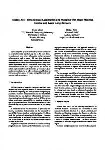
indeed counts on an advantageous ratio between mobile and static landmarks (or impacted cells) to estimate properly the ego-vehicle displacement. If some interesting works about an enhanced grid map [12] with three states (Occupied, Free, Not Known), about tracking data corresponding to mobile objects [13] or about combining SLAM algorithm with Multi-Hypothesis Tracking (MHT) solutions [14] have been proposed, the authors suggest that the probabilistic framework commonly used may not be explicit enough to deal with those crowded contexts. If it comes with a powerful mathematical background, the main limitations of using probability models are indeed illustrated in Fig. 1. This result has been obtained from the ML-SLAM solution developed at Inria [11], [15], [16].

Incoming vehicle Pedestrian False alarms

Fig. 1: Example of probabilistic SLAM Each impacted cell, through its occupancy probability, indeed conserves the information it has been impacted. A walking pedestrian or a moving vehicle for example leaves its path (i.e. its previous positions) in the recorded scans, and false alarms or ground impacts are kept recorded too. Even if thresholds or advanced mobile objects tracking could limit this problem, the SLAM assumption where laser impacts are generated by fix obstacles could be really tough to defend in crowded urban environment and so the system itself could lack precision and robustness. Those limits led the authors to switch from a probability framework to a more recent one: the Transferable Belief Model (TBM) introduced by Smets in 1994 [17]. The main advantage of this model over probabilities is indeed to represent knowledge in a way that fits really well with both grid map representation and laser data in a populated environment. The not-known is explicitly described and the

conflict management affords the possibility to deal with mobile objects and so to provide an obstacle free surrounding map of the vehicle which then fits with the SLAM assumption cited above. Moreover, TBM enables to keep the two kinds of information provided by a laser scan, i.e. the free area and the impacted objects. Using the particular example of SLAM for ITS and with data from a LIDAR, this article aims at proving that the approach of a Credibilist SLAM has been relevant and leads to interesting results and perspectives for the SLAM community. Since the TBM vocabulary did not yet find a standard, the authors named Credibilist this solution based on Credibility. The following article begins with a quick introduction to TBM and its application to grid map and laser data. The Credibilist SLAM algorithm is then described in Sec. III and a discussion around its matching operator is proposed in Sec. IV. The results and performances of the system are finally shown in the last section.

If this framework affords a more complete representation of the knowledge, it comes with a relatively important computational cost since the cardinality of the status to estimate increases from N to 2 N . However, in a reasonable context (N small), TBM is worth it due to its well adapted formalism to uncertainty. B. Data fusion in TBM In order to merge data from two distinct sources, the TBM framework distinguishes two main cases, depending whether the information provided can be trusted or not. For each case, the resulting BBA is computed using a combination rule: •

mΩ ∩ 2 (C) = 1

II. T RANSFERABLE B ELIEF M ODEL A. General overview The Transferable Belief Model (TBM) is an alternative to probabilities for knowledge representation based the evidence theory of Dempster and Shafer [18]. It is especially adapted to enhance the difference between uncertain and not-known. Given a set Ω of N hypotheses, also called frame of discernment, such as all these hypotheses are exclusive, a power set 2Ω is built as the set of all subset of Ω (including the empty set and Ω). ∀n ∈ [1, N ] Ω = {Hn } 2 = P(Ω) = {A|A ⊆ Ω} Ω

(1)

In the TBM framework, the union of hypotheses H n ∪Hm (∀n, m ∈ [1, N ], n = m) describes the lack of knowledge between those two hypotheses and the element ∅, called Conflict represents the part of contradictory information between sources. As a comparison, the complete description of the world proposed by probabilities for an hypothesis h and its com¯ would be Θ = {h, h} ¯ and a state of this world plementary h ¯ would be described by the two probabilities p(h) and p( h) ¯ such as p(h) + p(h) = 1. A contrario, the representation proposed by the TBM leads h, Ωhh¯ , ∅hh¯ }. A state of this world is to a power set 2Ω = {h, ¯ ¯ mΩ (Ω) then described by the four masses: m Ω (h), mΩ (h), Ω and m (∅). These four masses compose the Basic Belief Assignment (BBA), noted m Ω , such as:

mΩ (A) = 1

Conjunctive rule: If a source 1 and a source 2 are considered reliable, their BBA are combined using a conjunctive rule to build the resulting BBA m Ω ∩ 2 . By 1 definition:

(2)

A∈2Ω

The lack of knowledge or unknown between h and ¯h is explicitly described by the mass m Ω (Ω) and if two sources give contradictory information, then the conflict mass m Ω (∅) increases.

•

A∩B=C

Ω mΩ 1 (A).m2 (B)

∀A, B, C ⊂ 2Ω

(3) This rule is permissive because the combination merges both the certain and uncertain information. As an example, an empty BBA (m Ω 1 (Ω) = 1) merged with a categoric BBA on a singleton H (m Ω 2 (H) = 1) using a conjunctive rule leads to a categoric BBA on the same singleton H. Disjunctive rule: When only one of the sources is reliable, the resulting BBA m Ω ∪ 2 is computed using 1 a more restrictive rule: mΩ ∪ 2 (C) = 1

A∪B=C

Ω mΩ 1 (A).m2 (B)

∀A, B, C ⊂ 2Ω

(4) This rule is restrictive because only certain information is taken into account. The above example applied to a disjunctive rule indeed leads to an empty BBA. A lot of other combination rules can be found in the literature (e.g. [19],[20]) but this article focuses on those basic ones. C. Application to a grid map In the SLAM context, a grid map, also called occupancy grid, is a representation of an area discretized in cells. The information contained in a cell describes the confidence the system has in this cell to be occupied, knowing all the last measurements. This representation stand as a key point of the ML-SLAM process since each new measurement is compared to this grid to deduce the vehicle displacement. If this confidence has been firstly described as a single probability of occupation, different assertion on the cell state have then been proposed to enrich the grid description [14] or to reduce computational cost [12]. The idea of J. Moras et al. [21] to use an occupancy grid where each cell contained a BBA of the following power set (Eq. 5) is not completely new but the TBM framework

Filling the

that rules it provides an interesting background to deal with polar grid map mobile objects and ML-SLAM requirements. 2Ω = {F ree, Occupied, Ω, ∅}

Incoming vehicle Pedestrians behind the vehicle m Ω m Ω i,j,t (F ) = 1 i,j,t (Ω) = 1 Ω m i,j,t (O) = 1 m Ω i,j,t (∅) = 1 ego-position and heading

Fig. 2: Example of credibilist occupancy grid and conflict situations In the example shown in Fig. 2, the four focal elements of the chosen BBA could be seen in an occupancy grid. The F ree and U nknown areas surrounding the vehicle are well delimited and some impacted cells can be distinguished with there occupancy belief. Two main situations of conflict are also highlighted: when the laser beam meets a mobile object at a time and not at another time (An incoming vehicle or pedestrians in Fig. 2), or when the measurements are affected by false alarms (artefacts in Fig. 2). In both cases, the ability to model this knowledge is highly relevant and enriches the description of the surrounding world. D. Representation of laser data Being able with the TBM to describe uncertainty and lack of knowledge in the same formalism leads to a well adapted representation of laser data. Knowing that a laser beam provides both the information of an impacted cell and of all the free ones it crossed, a solution proposed in [21] is to fill a polar grid map by increasing the Occupied belief of an impacted cell and the F ree belief of the crossed ones (Fig. 3). For each cell of the polar grid map, defined by its angle θ ∼Ω and radius r, the measured BBA, noted mr,θ,t , is then filled as follow:

∼Ω

mr,θ,t (A) = λ ∼Ω mr,θ,t

(Ω) = 1 − λ

with A =

O if impacted F if crossed

with λ the confidence accorded to the LIDAR sensor.

Laser beam ∼Ω mr,θ,t ∼Ω mr,θ,t ∼Ω mr,θ,t

(5)

A cell in an unknown area is then described by an empty BBA while cells in explored areas have a BBA with either a focal element Occupied, F ree or if sources provide contradictory information, ∅. Since one of the SLAM goals is to estimate the BBA of a cell in the occupancy grid, this BBA is denoted m Ω i,j,t with i, j the cell position in the grid reference and t the considered time. The singleton hypothesis F ree and Occupied are respectively denoted F and O.

Impacted cells

(6)

(Ω) = 1 (F ) = 1 (O) = 1

Fig. 3: Filling the polar grid map with a new laser scan

III. C-SLAM C ONCEPT The C-SLAM concept is inspired by a SLAM solution used by Q. Baig et al. [16] and J. Xie et al. [15] and adapted to credibilistic occupancy grid. The main idea is to build at each iteration a grid with the incoming scan and to find the best match between it and the previously recorded grid map (Fig. 4). Polar grid map

Convertion to Cartesian coordinates ∼Ω

mi,j,t

Matching

Relative position and heading

Xt Merging Normalization

Occupancy grid

m Ω i,j,t−1

Fig. 4: Overview of the C-SLAM algorithm The best match also enables to obtain the displacement of the vehicle so that both its trajectory and the surrounding map are estimated in the same process. Since the displacement alone leads to a relative localization only, the considered reference in this article is the vehicle reference R 0 at the beginning of the experience. It means that at any time t, the position of the vehicle (x, y) and its heading θ are given relatively to the position and the heading at time t = 0. A. Conversion in Cartesian coordinates In order to search for a match between the polar grid obtained from the laser data and the previous occupancy grid saved in Cartesian coordinates, a conversion is required. To do so, a measured grid map is built by transforming the polar grid map in Cartesian coordinates (Fig. 5). The BBA of a cell ∼Ω from the resulting grid is denoted mi,j,t where the position (i, j) is the same as the corresponding cell in the occupancy grid. If this geometric transformation enables to match and later merge the two grids, it actually affects the measure so that further impacts will be duplicated and closer impact could be erased. If this characteristic cannot be avoided yet, its effects can be limited by choosing a compatible set of resolution for the polar and occupancy grids.

1 cell in polar grid = 1 cell in measured grid

1 cell in polar grid = 3 cells in measured grid

Applied to the SLAM context, this combination leads to estimate the BBA of each cell of the occupancy grid, knowing the new measured grid map. ∼Ω

∩ mi,j,t Ω m Ω i,j,t = m i,j,t−1

(8)

where m Ω i,j,t−1 is the BBA of a cell (i, j) in the occupancy ∼Ω

Polar grid sector Measured grid

grid reference and mi,j,t is the correspondent BBA in the measured grid map. Which leads to: ∼Ω m Ω (9) m Ω i,j,t (D) = i,j,t−1 (A). mi,j,t (B) A∩B=D

Fig. 5: Conversion from polar to Cartesian grid map

with D ⊂ Ω. m Ω i,j,t1

∩

B. Matching Once the polar grid map has been built, An a-priori state is computed based on the previous measurements and according to a basic Constant Speed model. X X 1 Δt . = . . (7) 0 1 X t|t−1 X t−1 state at time t in where Xt = (x, y, θ)t . is the vehicle . . . the reference R 0 and X .t = (x, y , θ)t its derivative at the . same time. (x, y) and ( x, y) are respectively the position and . velocity of the vehicle and θ and θ are the heading and the rotation speed. Δt is the time difference between times t and t − 1. On each component of the a-priori state X t|t−1 , a discrete uncertainty is applied to build a set of possible states that have to be tested (Fig. 6). Each so called candidates represents a possible evolution at time t knowing the state . Xt−1 and its derivative X t−1 at time t − 1. Each candidate then corresponds to a possible match between the measured grid map and the occupancy grid. Consequently, an operator is applied in order to score the candidate and find the best solution. A discussion on the choice of the operator is proposed in Sec. IV. .

θ t−1 .Δt Xt−1

Xt|t−1 .

y t−1 .Δt

Old state A-priori state Tested states

.

xt−1 .Δt

Fig. 6: Constant Speed model with a discrete uncertainty

C. Merging Considering both the measured grid map and the occupancy grid as reliable sources, J.Moras et al. [21] propose to use a conjunctive rule to assure the fusion between a new laser scan and the saved map as illustrated in Fig. 7.

∼Ω

m Ω i,j,t =

mi,j,t

Fig. 7: Merging step of the C-SALM algorithm based on [21]

D. Normalization with the conflict In addition, the proposition has been made in [21] to normalize the obtained map with the conflict mass m Ω i,j,t (∅). This operation, used with the conjunctive rule, has been proposed by Dempster and Shafer and is known as the orthogonal rule. It has the effect of distributing the belief from the conflict to the other focal elements of the BBA, according to their respective mass. Consequently, the focal element which gather the highest mass receives more importance. ⎧ Ω ⎨ m i,j,t (A) , if A = ∅ Ω (10) m i,j,t (A) = 1−m Ω i,j,t (∅) ⎩ 0, else In other words, if a conflict occurs by updating the map, the hypothesis with the highest belief will be strengthened. Knowing that the conflict is related to mobile objects in the environment or false alarms, this proposition enables to reduce the effect of such cases on the occupancy grid and so provides an obstacle free representation of the surrounding area of the vehicle (Fig. 8). If obstacle free is an on-purpose strong statement, it highlights that for a SLAM system, knowing that mobile objects lightly affect the matching step and so the mapping is a real advantage and serves the robustness of the system in crowded environment. IV. M ATCHING OPERATOR As introduced in the previous section, the key point of the proposed system lays in estimating the displacement in the matching process. This step is achieved by scoring each possible candidate

Merged occupancy grid

Normalized occupancy grid

the mass in the BBA so that a mobile object or an artefact is finally ignored. Consequently, a second solution would be the orthogonal rule (i.e. the conjunctive rule normalized by the conflict):

∼Ω

Ω OpC (m i,j,t−1 , mi,j,t ) =

m Ω i,j,t (F ) = 1

m Ω i,j,t (Ω) = 1

m Ω m Ω i,j,t (O) = 1 i,j,t (∅) = 1 ego-position and heading

Fig. 8: Effect of normalization by conflict on occupancy grid

around an a-priori position (cf Sec. III-B). Since each candidate represents a relative displacement between the measured grid and the occupancy grid, each cell from one grid is compared to its corresponding one in the other grid. This test on a pair of cell is completed by an operator on their respective BBA. The results of this operator for all the pairs are then summed to compute the global score of a candidate. Score =

∼Ω Op(m Ω i,j,t−1 , mi,j,t )

(11)

∀cells

The basic operators included in TBM has been introduced in Sec. II-B and if several operator inspired by the literature could have been used, only three has been chosen in this article to circle the most classic possibilities. A. Disjunctive operator Since the matching process aims at checking whether a displacement candidate and the previous occupancy grid could be merged or not, this candidate can be seen as a nonreliable source in the TBM framework. Until it has been elected, a candidate is indeed just a supposition so that the corresponding measured grid map remains uncertain. The combination rule adapted to this situation is the disjunctive one so the corresponding operator Op D is defined by: ∼Ω OpD (m Ω i,j,t−1 , mi,j,t )

=

∼Ω ∪ mi,j,t )(O) (m Ω i,j,t−1

(12)

In this case, only the focal element Occupied is considered in the BBA of the cells. Since the occupancy grid is normalized by the conflict, this theoretically means that only the fix obstacles are used in the match process. Consequently, this operator could be seen as a restrictive operator B. Disjunctive Orthogonal operator Another approach to match a candidate with the occupancy grid lays in using the same combination rule as the one used to update the occupancy grid (cf Sec. III-C). Since this rule includes a normalization by conflict (Sec. III-D), the singleton with the highest belief gathers the majority of

∼Ω

∩ mi,j,t )(O) (m Ω i,j,t−1

∼Ω

∩ mi,j,t )(∅) 1 − (m Ω i,j,t−1

(13)

However, this operator is permissive since all the cells in an unknown area, i.e. with an empty BBA, are considered. When it comes to the SLAM context, this could lead to major instability because the system would score equally a perfect match and a one which falls completely in an unknown area. In order to avoid this problem but conserve the normalization by conflict, all the masses on Ω in both sources are neglected. This leads to the following empirical operator Op OD : ∼Ω OpOD (m Ω i,j,t−1 , mi,j,t )

∼Ω

=

∪ mi,j,t )(O) (m Ω i,j,t−1

∼Ω

∩ mi,j,t )(∅) 1 − (m Ω i,j,t−1

(14)

C. Distance operator Even if the precision on laser impacts position is decreasing with their distance to the sensor, further impacted cells remain useful for better estimation of the heading angle. In order to emphasize this characteristic and use it for a better match, a last operator Op Dist which take the distance to the sensor into account is proposed. ∼Ω ∼Ω 2 2 OpDist (m Ω Ω i,j,t−1 , mi,j,t ) = OpOD (m i,j,t−1 , mi,j,t ). i + j (15) By multiplying the disjunctive orthogonal rule with the distance between the impact and the sensor, this operator indeed accords more importance to impacted cells far from the vehicle and can then theoretically reach a better rotation estimation. D. Other operators The authors have been tested too an operator that minimizes the conflict and another one that compares the free cells too. In the first case, the algorithm would lead to non-stable results in crowded environment (the conflict is basically high) and would still prefer to match with unknown area (no conflict). The second case is interesting but must be used with two average scores among all the cells (Score(F ) and Score(O)) that are then combined at the end of the process. In most cases, the number of free cells largely out passes the number of occupied cells so it could indeed ruins the quality of results and the robustness of the system to just sum the score all over the cells. An important remark is that this last method is much more greedy in terms of computational resources because of the number of cells to treat.

In order to compare the performances of the operators presented in Sec. IV, a particular set of sequences from the KITTI database has been selected on the following criteria: • One pursuit scenario. A car is driving at the same speed of the considered vehicle, about 30 m far ahead. • One large residential scenario with loops and turns • One crowded urban scenario. The results for each operator (Eq. 12, 14 and 15) and for each sequence are plotted in Fig. 9. By analysing only the pursuit scenario, it seems that the distance operator (Eq. 15) over passes the others. In this scenario, a vehicle is driving right ahead so that a lot of laser impacts are generated by this obstacle which is close to the laser sensor. As a matter of fact, all these impacts are not reliable for the operator distance so it reacts better than the other ones. However, if the result appears better, it is not because the operator considers these impacts not trustful but only because they are close so this result do not seem to be transposable. A look to the others results rapidly confirms that the pursuit is definitely the only good scenario for the operator distance. The two other scenarios indeed emphasize the quality of the operators disjunctive and disjunctive orthogonal over the operator distance. The operator disjunctive (Eq. 12) only differs from the operator disjunctive orthogonal (Eq. 14) by its consideration of the conflict cells. Where it do not consider those case at all, the disjunctive orthogonal are weighting them so that conflict situations are considered according to their confidence. If this difference doest not impact a lot the presented results, the operator disjunctive orthogonal is preferred because it appeared to be more robust when tested in numerous scenarios. The following results are then obtained using the operator presented in Sec. IV-B (Eq. 14). C. Performances In order to visualize the output position and heading provided by the credibilist SLAM algorithm, three complete sequences are plotted in Fig. 10.

Translation error [m]

5 0 0

Rotation error [deg] Translation error [m]

B. Operator Comparison

Op. Disjunctif Op. Disjunctif Orthogonal Op. Disjunctif Distance

50

100

150 Iteration

200

250

300

Rotation errors 2


1 0 0

50

100

150 Iteration

200

250

300

Translation errors 100


50 0 0

Rotation error [deg]

All the tests presented in this article have been managed by using the KITTI dataset available online [22]. Since this database has been built with data from a Velodyne, a 2D laser scan is extracted from each data set in order to simulate a simple layer LIDAR with a field of view of 360 degrees and a resolution of 0.09 degrees. This method can obviously be criticized but it enables to have a direct comparison between the SLAM output and the ground truth in term of displacement and mapping. If no contradictory information are mentioned, the resolutions of the occupancy grid is 20 cm and the ones in the polar grid maps are 20 cm and 0.5 degrees.

Translation error [m]

A. KITTI Dataset


500

1000

1500 Iteration

2000

2500

3000

Rotation errors 20


10 0 0

500

1000

1500 Iteration

2000

2500

3000



10 5 0 0

Rotation error [deg]

V. R ESULTS

200

400

600 Iteration

800

1000

1200

Rotation errors 6


4 2 0 0

200

400

600 Iteration

800

1000

1200

Fig. 9: Translation and rotation errors plotted for each operator along three sequences (Top: a pursuit scenario; Middle: a long urban scenario; Bottom: a crowded urban scenario)

The first two plots correspond to a 3.7 and a 2.2 kilometres test drive in a classic urban environment. Their respective errors in translation at the end of the path are 11.1 and 29.5 meters, i.e. 0.3% and 1.3% of the total path. Concerning the rotation error, their values when the sequence ends are respectively 6.7 and 6.2 degrees. The last example is a semi-urban 1.7 km path passing by a residential zone up on a hill. It implies a variable altitude and even with the 2D C-SLAM and with a single layer LIDAR, the translation error at the end is limited to 4.8% and the rotation one to 15.1 degrees. If these plots enable to weight the performances of C-SLAM on off-line data, it is worth to notice that the complete presented algorithm runs in less than 100 ms on a laptop equipped with a dual core processor running at 2.8 GHz and

300 200 100 Probabilist grid

Y (m)

Credibilist grid

0 −100 −200 Measured position Ground truth

−300 0

100

200 300 X (m)

400

500

35

300

30 25 Y (m)

200

Y (m)

100

15 10 5

0

Credibilist SLAM Ground truth Probabilistic SLAM

0 160

−100

Measured position Ground truth 0

100 200 X (m)

300

170

180

190 200 X (m)

210

220

230

Fig. 11: Comparison between credibilist and probabilist SLAM in a crowded urban environment

−200 −300 −100

20

400

D. Odometry drift 100

Y (m)

0 −100 −200 −300 Measured position Ground truth

−400 −100

0

100

200 300 X (m)

400

500

600

Fig. 10: Total path for three representative scenarios

with the laser set-up describe in Sec. V-A. Even without any loop closure and additional sensors, these results are really promising and enhances the possibilities of the TBM framework in terms of precision and reliability. In addition, Fig. 11 proposes a comparison between probabilistic and credibilistic SLAM in a crowded town center. The two algorithms have exactly the same architecture so that they differ only with their mathematical framework : credibility versus probability. If their is a slight advantage for the credibilist solution in terms of localisation (error of 0.3% against 2.0% of the total path), its map representation appears clearer and leads to an explicit description of the complex environment surrounding the vehicle.

Since SLAM is a relative localization method. A drift is generated from the accumulation of errors over the time. If this drift can be limited or corrected by fusion with others sensors, it is worth to quantify it for the Credibilist SLAM system alone. The method proposed for the KITTI odometry benchmark is adapted in this article to score the proposed SLAM (which is 2D). For each ten iterations (each second) of a sequence, eight errors in translation and rotation, if it is possible, are computed following this rule:

T rue Measured . − ΔXt,t Xerror (t, d) = ΔXt,t d d

(16)

i with ΔXt,t = Xti − Xtid and td is the time at which the d vehicle have driven the distance d from its position at time t and d ∈ {100, 200, ..., 800}. T rue and M easured are respectively denoting the Ground Truth and the Measured state of the vehicle in the reference R0 introduced in Sec. III. For each iteration and distance, X error is collected over 10 sequences of the KITTI database and a mean per distance is then computed to reach the corresponding translation and rotation errors (or drift) of the system. These 10 sequences contain urban scenarios as well as countryside ones with different difficulties such as open field, hills, small or curved roads, corridors or pursuits. Results are plotted in Fig. 12. Fig. 12 enables to note that the drift in translation is between 2% et 4.5% with a mean score at 3.2% and that the drift in rotation is between 0.0028deg/m and 0.0072deg/m with a mean score at 0.0040deg/m. As a comparison, the DEMO solution [23] based on a fusion between vision and laser data from the complete velodyne scan reaches a translation error score of 1.14%

Rotation error [deg/m] Translation error [%]

R EFERENCES

Translation errors (score: 3.20 %) 5 4 3 2 100

200

400 500 Path length [m]

600

700

800

700

800

Rotation errors (score: 0.0040 deg/m)

−3

8

300

x 10

6 4 2 100

200

300

400 500 Path length [m]

600

Fig. 12: Translation and rotation errors for 10 sequences of KITTI database

and a rotation error score of 0.0049deg/m for the same time performances but on another set of sequences. As explained above, Fig. 12 represents a mean over several sequences. However, it is worth to notice that the best sequence leads to drift scores of 1.48% for the translation and 0.0017deg/m for the rotation. Even if it concerns only a particular sequence, this result is really encouraging knowing that it is based only on a simple layer LIDAR scans.

VI. C ONCLUSION This article has introduced a new SLAM algorithm by using Maximum Likelihood methods in a TBM framework. The proof has been made that this technique has good performances and is well adapted to a SLAM context using a LIDAR sensor. If a simple evolution model has been used to compute the a-priori state and the uncertainty on it, it would be worth to upgrade the algorithm with a more robust and precise one such as the one provided by classical Kalman or particle filters. But above all, the proposition truly opens a large field of perspectives for the SLAM community because all the current and past research ideas can be adapted to the TBM in order to have a SLAM robust to crowded environment. Using a pre-recorded map, implementing a loop closure system, merging information from a navigation map, fusing data from other sensors or testing other operators are ideas among all the possibilities that could be re-thought in a credibilist framework. To conclude, it is worth to highlight the obstacle free map that has been built via the Credibilist SLAM process and that could be used by other ITS algorithm. This representation is possible only because the system represents moving obstacles by the conflict. A SLAM and Mobile Objects Tracking (SLAMMOT) system is so already engaged without any additive computational cost.

[1] H. F. Durrant-Whyte and T. Bailey, “Simultaneous localization and mapping: part I,” Robotics & Automation Magazine, IEEE, vol. 13, no. 2, pp. 99–110, 2006. [2] T. Bailey and H. F. Durrant-Whyte, “Simultaneous localization and mapping (SLAM): Part II,” Robotics & Automation Magazine, IEEE, vol. 13, no. 3, pp. 108–117, 2006. [3] S. Thrun, “Robotic mapping: A survey,” Exploring artificial intelligence in the new millennium, pp. 1–35, 2002. [4] O. El Hamzaoui and B. Steux, “A fast scan matching for grid-based laser SLAM using streaming SIMD extensions,” 11th International Conference on Control Automation Robotics & Vision (ICARCV 2010), pp. 1986–1990, 2010. [5] G. Grisetti, R. Kümmerle, C. Stachniss, and W. Burgard, “A Tutorial on Graph-Based SLAM,” Intelligent Transportation Systems Magazine, IEEE, vol. 2, no. 4, pp. 31–43, 2010. [6] J. Folkesson and H. Christensen, “Graphical SLAM - a self-correcting map,” IEEE International Conference on Robotics and Automation, 2004. Proceedings. ICRA ’04, vol. 1, pp. 383–390 Vol.1, 2004. [7] J. Oberländer, A. Roennau, and R. Dillmann, “Hierarchical SLAM Using Spectral Submap Matching with Opportunities for Long-Term Operation,” 2013 IEEE International Conference on Advanced Robotics, 2013. [8] T.-D. Vu, “Vehicle perception: Localization, mapping with detection, classification and tracking of moving objects,” Ph.D. dissertation, Institut National Polytechnique de Grenoble (INPG), 2009. [9] C.-C. Wang and C. E. Thorpe, “Simultaneous localization and mapping with detection and tracking of moving objects,” IEEE International Conference on Robotics and Automation, 2002. Proceedings. ICRA ’02., vol. 3, pp. 2918–2924, 2002. [10] M. Montemerlo, S. Thrun, D. Koller, and B. Wegbreit, “FastSLAM: A factored solution to the simultaneous localization and mapping problem,” in AAAI/IAAI, 2002, pp. 593–598. [11] J. Xie, F. Nashashibi, M. Parent, and O. G. Favrot, “A real-time robust global localization for autonomous mobile robots in large environments,” 11th International Conference on Control Automation Robotics & Vision (ICARCV 2010), pp. 1397–1402, 2010. [12] B. Steux and O. El Hamzaoui, “tinySLAM: A SLAM algorithm in less than 200 lines C-language program,” pp. 1975–1979, 2010. [13] D. Hahnel, R. Triebel, W. Burgard, and S. Thrun, “Map building with mobile robots in dynamic environments,” pp. 1557–1563 vol.2, 2003. [14] D. Meyer-Delius, M. Beinhofer, and W. Burgard, “Occupancy Grid Models for Robot Mapping in Changing Environments.” in AAAI, 2012. [15] J. Xie, F. Nashashibi, M. Parent, and O. Garcia-Favrot, “A realtime robust SLAM for large-scale outdoor environments,” ITS World Congress, 2010. [16] Q. Baig, T.-D. Vu, and O. Aycard, “Online localization and mapping with moving objects detection in dynamic outdoor environments,” in IEEE 5th International Conference on Intelligent Computer Communication and Processing, 2009. ICCP 2009. IEEE, 2009, pp. 401–408. [17] P. Smets and R. Kennes, “The transferable belief model,” Artificial intelligence, vol. 66, no. 2, pp. 191–234, 1994. [18] G. Shafer, A mathematical theory of evidence. Princeton university press Princeton, 1976, vol. 1. [19] E. Lefevre, O. Colot, and P. Vannoorenberghe, “Belief function combination and conflict management,” Information Fusion, vol. 3, no. 2, pp. 149–162, Jun. 2002. [20] E. Ramasso, “Reconnaissance de séquences d’états par le Modèle des Croyances Transférables. Application a` l’analyse de vidéos d’athlétisme.” Ph.D. dissertation, Université Joseph Fourier de Grenoble, 2007. [21] J. Moras, V. Cherfaoui, and P. Bonnifait, “Credibilist occupancy grids for vehicle perception in dynamic environments,” IEEE International Conference on Robotics and Automation (ICRA 2011), pp. 84–89, 2011. [22] A. Geiger, P. Lenz, and R. Urtasun, “Are we ready for autonomous driving? The KITTI vision benchmark suite,” IEEE Conference on Computer Vision and Pattern Recognition (CVPR 2012), pp. 3354– 3361, 2012. [23] J. Zhang and S. Singh, “DEMO: Depth Enhanced Monocular Odometry,” 2013.