Landmark-based Simultaneous Localization and Mapping with Stereo Vision Matthew N. Dailey
Manukid Parnichkun
Sirindhorn International Institute of Technology Thammasat University Pathumthani, Thailand 12121
[email protected]
Mechatronics Asian Institute of Technology Pathumthani, Thailand 12120
[email protected]
Abstract— SLAM, the problem of a mobile robot building a map of its environment while simultaneously having to determine its location within that map, is one of the current fundamental challenges of robotics. Although a great deal of success has been achieved with laser range finders as sensors and a planar world assumption, low-cost commercial robots will benefit from robust SLAM using cameras only. Towards the goal of a robust, six degree-of-freedom, vision-based SLAM algorithm, we describe the application of “FastSLAM” [1] to the problem of estimating a map from observations of 3D line segments using a trinocular stereo camera rig. By maintaining not only multiple hypotheses about the robot’s position in space, but also maintaining multiple maps corresponding to those possible position hypothesis, the algorithm has the potential to overcome the systematic map errors induced by incorrect correspondence estimation.
I. I NTRODUCTION Simultaneous localization and mapping (SLAM) is one of the most active areas in mobile robotics research. The task is to construct a metric map of the robot’s workspace from noisy sensor readings, while simultaneously estimating the robot’s location from the partial map and noisy odometry measurements. The difficulty of the SLAM problem depends on the characteristics of the robot’s environment, the characteristics of its sensors, and the level of map detail required by the application. The environment could be relatively benign, say, if it is indoors with flat floors and good traction for robot wheels. But it could also be quite subversive, for instance, in the case of aircraft and submarines. The most common sensors in use today are laser range finders and video cameras. Lasers have some key benefits: they are accurate and provide range information directly. However, they are heavy, expensive, and primarily twodimensional (although, of course, more than one plane could in principle be scanned). Cameras, on the other hand, are lightweight, small, and cheap, but are fairly difficult to work with. In particular, extracting range information from cameras normally requires triangulation from multiple perspectives or a great deal of prior knowledge. The last characteristic, the level of detail required by the application, could be fairly coarse. In the case of a robotic wheelchair whose job is to get its occupant from place to place in a home, the detailed shape and size of pieces of furniture would probably not be relevant. But other applications
would require an enormous amount of accurate detail in their maps. Imagine an autonomous land mine detector operating in a dense jungle. This robot would not only have to make certain that not a single square foot of jungle is missed, but would also require extremely detailed knowledge of the many obstructions preventing it from navigating between points. To date, the majority of SLAM research has focused on two-dimensional maps acquired from laser range scanning. Several successful systems have been demonstrated; most use either a 2D occupancy grid [2], [3] or a database of landmarks in the plane [1], [4]. We are primarily interested in building real-time, visionbased SLAM systems for complex environments requiring motion estimates with 6 degrees of freedom. As for laserbased systems, the common choices for vision-based mapping are again either occupancy grids or landmark databases. But now we are dealing with 3D occupancy grids and databases of 3D landmarks. Although 3D volumetric grids have been shown to make realistic, detailed maps [5], [6], they require a prohibitive amount of memory and processing for large-scale environment mapping. So here we focus on SLAM algorithms for learning of 3D landmark databases from video data. Zhang and Faugeras [7] were among the early pioneers in this area. Using mobile robots equipped with trinocular stereo camera rigs, they were able to successfully map small indoor environments. They modeled the world as a collection of straight line segments and tracked the lines’ positional uncertainty with Kalman filters. Se, Lowe, and Little [8] demonstrate the use of SIFT (scale invariant feature transform) point features as landmarks for the SLAM problem. They also used a trinocular stereo camera rig, and modeled the positional uncertainty of the landmarks with Kalman filters. Davison, Cid, and Kita [9] demonstrate a single-camera SLAM algorithm capable of learning a set of 3D point features. Their algorithm uses an ingenious mix of particle distributions with the extended Kalman filter to overcome the initial range uncertainty arising from the use of only one camera. All of the vision-based approaches estimate camera motion (either with or without the help of odometry) then update a map. Motion estimation and map updating both depend critically on solving a correspondence problem, either between
features in successive camera frames or between observed features and map features. This is clearly a problem when ambiguities lead to correspondence errors. If erroneous correspondences are used to estimate motion, motion estimates can be thrown off, causing the map to be updated from an incorrect position, in turn leading to systematic drift in the map. In a series of recent papers (summarized in [1]), Montemerlo, Thrun, and colleagues have proposed an interesting way around this same problem for laser range finder-based SLAM systems. The idea is to maintain multiple possible maps corresponding to multiple possible data association hypotheses. Their algorithm, “FastSLAM,” uses a particle filter for sampling from the space of possible robot paths, but unlike previous systems based on particle filters (e.g. [3]), each particle maintains its own map. The new approach yields impressive results in mapping a large outdoor environment, and with appropriate optimization, is suitable for real-time implementation. In this paper, we explore the possibility of using a similar approach to maintain multiple correspondence hypotheses in the realm of 3D visual landmark-based SLAM. The landmarks in our case are 3D line segments obtained from a trinocular stereo vision system. We find that the method is indeed capable of maintaining the robot’s location while constructing a consistent landmark map. II. L ANDMARK - BASED SLAM WITH STEREO VISION Following [1], our algorithm maintains at time t a set of particles, each representing a possible robot path from time 0 to time t. Associated with each particle is a candidate position st for the robot at time t and a map, represented as a k-D tree of landmarks with associated Gaussian uncertainties. In our system, after each robot motion ut , a set of trinocular stereo images is captured, and a set zt of landmark measurements (line segments) is extracted from those images. These line segment measurements, along with the measured motion ut , are used to update each particle’s map and position estimate. A. Landmark extraction Our algorithm assumes a calibrated stereo camera rig with three pinhole cameras. To simplify matching, we further assume that the three cameras share the same image plane, that the first and second cameras are rectified so that the epipolar lines correspond to the same rows in each image, and that the first and third cameras are rectified so that the epipolar lines correspond to the same columns in each image. a) 2D line segment extraction: The basic 2D feature in our system is the line segment. We extract line segments using Canny’s method [10] following the implementation in VISTA [11]. The edge detector first performs nonmaxima suppression, links the edge pixels into chains, and retains the strong edges with hysteresis. Once edge chains are extracted from the image, we approximate each chain by a sequence of line segments. Short line segments, indicating edges with high curvature, are simply discarded in the current system.
b) Stereo matching: We use a straightforward stereo matching algorithm similar to the approach of [7]. For each line segment in the reference image, we compute the segment’s midpoint, then consider each segment intersecting that midpoint’s epipolar line in the second image. Segments not meeting line orientation and disparity constraints are discarded. Each of these potential matches determines the location and orientation of a segment in the third image. If such a consistent segment is indeed found in the third image, the potential match is retained; otherwise it is discarded. If at the end of this process, we have one and only one consistent match, we assume it correct; otherwise, the reference image line segment is simply ignored. c) 3D line representation: Now our goal is to estimate a three-dimensional line from the three observed twodimensional lines. As we shall see in the next section, each landmark in our map is represented by a point with an associated Gaussian uncertainty. Furthermore, landmark positions and uncertainties are updated using the Kalman filter update rule. Since the Kalman filter update requires inversion of the measurement covariance matrix, the most straightforward approach is to use a minimal 3D line representation. In particular, we represent a line as a 4-vector L = (θ, φ, r, ρ)T , where, assuming P is the projection of the origin onto L, the parameters θ, φ, and r describe P in spherical coordinates, and ρ is the rotation of L around the line through the origin and P . d) 3D line estimation: Since 2D lines have two intrinsic parameters and 3D lines have four intrinsic parameters, we have 6 independent nonlinear equations in four unknowns. Assuming Gaussian measurement error in the image, maximum likelihood estimation of the 3D line’s parameters becomes a nonlinear least squares problem, which we solve with Levenberg-Marquardt minimization [12]. As an initial estimate of the line’s parameters, we use the 3D line (uniquely) determined by two of the 2D measurements. e) Error propagation: Through each step of the 3D line estimation process, we maintain explicit Gaussian error estimates. We begin by assuming spherical Gaussian measurement error in the image with a standard deviation of one pixel. Arranging the n (x, y) coordinates of the pixels in a line as a column vector x, the covariance of x is simply Σx = I2n×2n . Since the vector of parameters l describing the 2D line best fitting x is a nonlinear function l = f (x), the covariance of l ∂f evaluated is Σl = JΣx J T , where J is the Jacobian matrix ∂x at x. ˆ = The maximum likelihood estimate of the 3D line L T (θ, φ, r, ρ) obtained from the three 2D line segments l = (l1 , l2 , l3 ) is clearly not a simple function, since it is computed by an iterative optimization procedure. However, if l = f (L) is the function mapping from the parameter space to the ˆ is a measurement space, it turns out that, to first order, L random variable with covariance matrix (J T Σl J)−1 , where ∂l [13]. J is the Jacobian matrix ∂L f) Numerical stability: Unfortunately, the minimal 4parameter representation of 3D lines leads to covariance ma-
trices that are very nearly singular, creating numerical stability problems. To understand the issue, consider a horizontal line on the ground one meter to the right of the robot, running parallel to the robot’s line of sight. If the line is observed at a distance of 10 meters, a small error in our estimate of the direction of that line translates to a large error in our estimate of r, the length of the projection of the origin (the robot’s position) onto the line. At the same time, that small error in estimating the orientation of the line translates to a very small error in θ, the rotation in the plane of the projection of the origin onto the line. This situation means our error ellipses tend to be quite elongated with high condition numbers. To prevent numerical problems when the covariance matrices are inverted, we enforce constraints on the condition number and minimum singular value of each covariance matrix. In particular, we let U SU T be the singular value decomposition of the positive definite covariance matrix Σ. If σ1 is the largest singular value of Σ, and σn is the smallest singular value of Σ, we construct an adjusted singular value matrix S 0 by adding to each of the singular values σi the smallest nonnegative quantity λ guaranteeing that the smallest adjusted singular value σn0 = σn + λ is above a small threshold and that the new condition number σ10 /σn0 is below another threshold. We then replace Σ with the better-conditioned matrix U S 0 U T . g) Line transforms: Once the four-dimensional representation of an observed 3D line is estimated from a trinocular line correspondence, it is necessary to transform that line from camera coordinates into robot coordinates, since the reference camera is in general translated and rotated relative to the robot itself. It is also necessary to transform landmarks from robot coordinates into world coordinates, when the robot’s position is determined, for instance, and from world coordinates back to robot coordinates, when a landmark in the map is considered as a possible match for an observed (robot coordinate) landmark. In each of these cases, the transformed line L0 = t(L) is computed as a nonlinear function of the original line, and the transformed line’s covariance is propagated by ΣL0 = JΣL J T , where J is the Jacobian matrix ∂t ∂L evaluated at L. B. Particle update Here we follow Montemerlo and colleagues’ “FastSLAM 1.0” algorithm [1], adapted to the case of line segments as landmarks. FastSLAM’s goal is to estimate the posterior p(st , Θ | z t , ut , nt ) where st is the robot’s path from time 0 to time t, Θ is the map (a list of landmark positions and covariances), z t is the set of observed landmarks from time 0 to t, ut is the robot’s assumed motion from time 0 to t, and nt is the set of correspondences between the observed features z t and stored features θ t in the map. FastSLAM is efficient, despite estimating a posterior over the robot’s path from time 0 to t, because the posterior can
be factored p(st , Θ | nt , z t , ut ) = p(st | nt , z t , ut )
N Y
p(θn | st , nt , z t )
n=1
since the individual feature estimates in the map are conditionally independent given the robot’s path and a correspondence between map features and observations. In FastSLAM, the distribution p(st | nt , z t , ut ) is approximated by a particle filter. Each particle in the filter represents one possible robot path st from time 0 to t. Since the map feature estimates p(θn | st , nt , z t ) themselves depend on the robot path, each particle also carries with it an extended Kalman filter (EKF) for each of the landmarks in the map. Here we provide a capsule summary of the FastSLAM algorithm as adapted to our system. For details of FastSLAM, the reader should refer to [1]. At each time step t, the robot performs an action ut , captures a set of images, and extracts a set of 3D line segments zt from the image set as described in section II-A. Each particle m in the particle filter is then updated with the new robot action ut and zt as follows: 1) Using the particle’s previous state estimate st−1 , we draw a sample st from the motion model p(st | st−1 , ut ), which is approximated by a Gaussian distribution around the position sˆt we would obtain if the robot exactly performed action ut from position st−1 . 2) Assuming the sampled position st , for each observed landmark zti , we find the most likely correspondence with a stored landmark, i.e. ˆ t−1 , st , z t−1 , ut ) n ˆ ti = arg max p(zti | nti , n nti
3) For each observed landmark, if the probability of the observation given the most likely correspondence p(zti | n ˆ ti , n ˆ t−1 , st , z t−1 , ut ) is below threshold, we add it to the map as a new landmark. If the probability is above threshold, we combine the new observation with the old landmark position estimate using the extended Kalman filter update equation. 4) Over all the observed landmarks, we calculate the [m] importance weight wt , assuming conditional independence of the individual observations zti : Y [m] wt = p(zti | n ˆ ti , n ˆ t−1 , st , z t−1 , ut ) i
After the particles are updated, we then resample the particles, with replacement, proportional to the importance weights calculated in step 4. above. The updated particles with large weights, indicating a high degree of consistency between observed and stored landmarks, are more likely to survive the resampling step than those particles with small weights, indicating less consistency between observed and stored landmarks. III. E XPERIMENTAL METHODS We tested the vision-based SLAM algorithm in simulation with a virtual robot moving through a virtual world, rendered with OpenGL from a VRML model. Our simulator allows
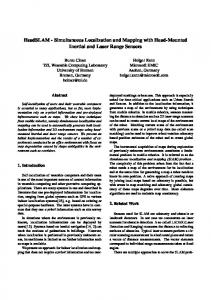
us to test localization and mapping algorithms in arbitrarily complex environments, with a known ground truth (the VRML model itself). We plan to release this simulator as open source software in the near future. For our SLAM experiments, we chose as an environment a publically-available 3D model of Housestead’s fort, a Roman garrison from the 3rd century A.D. on Hadrian’s Wall in Britain [14]. A sample view from our virtual trinocular stereo rig is shown in Figure 1. This environment is an interesting test of vision-based SLAM algorithms because, on the one hand, it generates many long, strong, straight edges that should be useful for localization. On the other hand, it is highly textured, creating a large number of edges, and the textures are highly repetitive in many places, leading to many ambiguities for correspondence algorithms. We teleoperated our virtual robot through this virtual world in a long loop of about 300m. At approximately 1m intervals, the virtual camera rig was instructed to capture a set of stills from its three cameras. To make the problem more challenging, we simulated the effects of a traveling on a rough outdoor surface, so that the robot’s vertical (Z) position varied approximately ±0.04m from 0, its pitch and roll varied ±2.5 degrees from 0, and its yaw varied ±3 degrees from its expected course. To enable the robot to view a large portion of the nearby environment, while also accurately estimating the depth of objects at reasonable distance, we used a fairly long stereo baseline (1m) and a fairly wide angle lens (70 degrees horizontal field of view). A more realistic setup achieving similar accuracy would require using more than one camera rig with narrow fields of view and more narrow baselines. We plan to release the data set with ground truth to interested researchers via the WWW. IV. R ESULTS We report the results of three experiments here. First, to determine whether the 3D line segment sensor is accurate enough to support map building assuming known positions, we ran the mapping algorithm as described earlier, but with the known “true” simulated robot positions rather than the positions estimated by the SLAM algorithm. This resulted in a 3D line map whose projection into the plane is shown in Figure 2(a). In a second experiment, we sought to obtain a lower bound on performance. We ran the mapping algorithm as described, but rather than estimating the robot’s position from sensor data, we simply assumed the robot motions as described by the simulated odometry measurements were correct. This resulted in an extremely bad 3D map, whose projection into the plane is shown in Figure 2(b). Clearly, this map would be nearly useless for navigation. In the final, third experiment, we ran our adaptation of FastSLAM on the same sensor data. We used 100 particles, each estimating the robot’s position with 6 degrees of freedom. The result of one run is shown in Figure 2(c). Although
the map is far from the “perfect” map of Figure 2(a), it is clear that the SLAM algorithm enables recovery from some of the distortions caused by bad odometry data in Figure 2(b). V. C ONCLUSION In this paper, we have shown that Thrun, Montemerlo, and colleagues’ FastSLAM algorithm, originally designed for 2D laser-based SLAM, is quite feasible for vision-based SLAM with 3D lines as landmarks. With the help of a straightforward line segment correspondence algorithm, the trinocular stereo camera sensor produces 3D landmarks suitable for use by FastSLAM’s particle filter for weighting the importance of sampled robot positions. By maintaining multiple robot path hypotheses and a separate maximum likelihood map for each hypothesized path, the algorithm can potentially overcome the thorny problem of systematic error induced by erroneous correspondences. However, there are serious issues to address. With a good 3D line representation and a sufficiently large number of particles in the filter, it should be possible to achieve, very nearly, the “perfect” map shown in Figure 2(a). The main problem is that in its current implementation, our algorithm is too slow. The run time is dominated by particle update step 2), namely the determination of the most likely correspondence for an observed landmark. This is partially due to the fact that we do not currently attempt to keep the k-D trees storing our landmark databases balanced, but even more so due to the fact that the measurement error for the 4-dimensional representation of 3D lines tends to be large, for the same reasons causing the numerical instability in Section II-A. This means that a large fraction of landmarks in the k-D tree must be considered as potentially corresponding features, and the full comparison is fairly expensive. The large number of observation-map feature comparisons in turn limits the number of particles we can use while maintaining a run time within range of real time performance. Thrun et al. [1] cite good performance for their FastSLAM 1.0 algorithm with 100 particles, but their problem is only a 3 degree of freedom problem, whereas ours is a 6 degree of freedom problem, most likely requiring far more particles to achieve similar performance. With these issues in mind, in our current research, we are currently exploring better 3D line representations, as well as the use of Montemerlo, Thrun, and colleagues’ “FastSLAM 2.0” algorithm, which promises a dramatic decrease in the number of particles necessary by focusing the particle filter’s proposal distribution in regions more likely to be consistent with the observed sensor measurements. ACKNOWLEDGMENTS This research was supported by Thailand Research Fund (TRF) grant MRG4780209 to MND. Some of the simulation software used in this project was donated by Vision Robotics Corporation of San Diego, CA USA. We are grateful to Thavida Maneewarn for suggestions on covariance matrix regularization.
(a) Fig. 1.
(b)
(c)
Sample trinocular image set captured in simulation. (a) Reference image. (b) Horizontally aligned image. (c) Vertically aligned image. 140 120 100 80 60 40 20 0 −20 −40 −200
−150
−100
−50
0
50
100
(a) 150 140
120
100
100 80
60
40
50
20
0
0 −80
−60
−40
−20
0
(b)
20
40
60
−20 −80
−60
−40
−20
0
20
40
60
80
(c)
Fig. 2. Mapping results for Housestead’s fort. (a) 2D projection of the 3D map obtained with perfect localization. (b) Raw map obtained assuming the location predicted by odometry. (c) Map estimated by the vision-based SLAM algorithm.
R EFERENCES [1] S. Thrun, M. Montemerlo, D. Koller, B. Wegbreit, J. Nieto, and E. Nebot, “FastSLAM: An efficient solution to the simultaneous localization and mapping problem with unknown data association,” Journal of Machine Learning Research, 2004 (in press). [2] S. Thrun, D. Fox, W. Burgard, and F. Dellaert, “Robust Monte Carlo localization for mobile robots,” Artificial Intelligence, vol. 128, no. 1–2, pp. 99–141, 2001. [3] S. Thrun, W. Burgard, and D. Fox, “A real-time algorithm for mobile robot mapping with applications to multi-robot and and 3D mapping,” in IEEE Conference on Robotics and Automation, vol. 1, 2000, pp. 321–328. [4] G. Dissanayake, P. Newman, S. Clark, H. Durrant-Whyte, and M. Csorba, “A solution to the simultaneous localization and map building (SLAM) problem,” IEEE Transactions on Robotics and Automation, vol. 17, no. 3, pp. 229–241. [5] H. Moravec, “DARPA MARS program research progress: Robust navigation by probabilistic volumetric sensing,” Carnegie Mellon University, Tech. Rep., 2002, http://www.ri.cmu.edu /∼hpm/project.archive/robot.papers/ 2002/ARPA.MARS/Report.0202.html. [6] M. Garcia and A. Solanas, “3D simultaneous localization and modeling from stereo vision,” in IEEE Conference on Robotics and Automation, 2004, pp. 847–853. [7] Z. Zhang and O. Faugeras, 3D Dynamic Scene Analysis. SpringerVerlag, 1992. [8] S. Se, D. Lowe, and J. Little, “Mobile robot localization and mapping with uncertainty using scale-invariant visual landmarks,” The International Journal of Robotics Research, vol. 21, no. 8, pp. 735–758, 2002. [9] A. Davison, Y. Cid, and N. Kita, “Real-time 3D SLAM with wideangle vision,” in Proceedings of the IFAC Symposium on Intelligent Autonomous Vehicles, 2004. [10] J. Canny, “A computational approach to edge detection,” IEEE Transactions on Pattern Analysis and Machine Intelligence, vol. 8, no. 6, 1986. [11] A. Pope and D. Lowe, “Vista: A software environment for computer vision research,” in IEEE Conference on Computer Vision and Pattern Recognition, 1994. [12] W. Press, B. Flannery, S. Teukolsky, and W. Vetterling, Numerical Recipes in C. Cambridge: Cambridge University Press, 1988. [13] R. Hartley and A. Zisserman, Multiple View Geometry in Computer Vision. Cambridge, UK: University Press, 2000. [14] B. B. Corporation, “Housestead’s fort (3d model),” 2004, http://www.bbc.co.uk/ history/3d/houstead.shtml.