Int. J. Data Mining and Bioinformatics, Vol. 16, No. 1, 2016
Cross-validation and cross-study validation of chronic lymphocytic leukaemia with exome sequences and machine learning Abdulrhman Aljouie Department of Computer Science, New Jersey Institute of Technology, Newark, NJ 07102, USA Email:
[email protected]
Nihir Patel and Bharati Jadhav Department of Genetics and Genomics Sciences, Icahn School of Medicine at Mount Sinai Hospital, Hess Center for Science and Medicine, New York City, NY 10029, USA Email:
[email protected] Email:
[email protected]
Usman Roshan* Department of Computer Science, New Jersey Institute of Technology, Newark, NJ 07102, USA Email:
[email protected] *Corresponding author Abstract: The era of genomics brings the potential of better DNA-based risk prediction and treatment. We explore this problem for chronic lymphocytic leukaemia that is one of the largest whole exome data set available from the NIH dbGaP database. We perform a standard next-generation sequence procedure to obtain Single-Nucleotide Polymorphism (SNP) variants and obtain a peak mean accuracy of 82% in our cross-validation study. We also cross-validate an Affymetrix 6.0 genome-wide association study of the same samples where we find a peak accuracy of 57%. We then perform a cross-study validation with exome samples from other studies in the NIH dbGaP database serving as the external data set. There we obtain an accuracy of 70% with top Pearson ranked SNPs obtained from the original exome data set. Our study shows that even with a small sample size we can obtain moderate to high accuracy with exome sequences, which is encouraging for future work. Keywords: exome wide association study; chronic lymphocytic leukaemia; machine learning; disease risk prediction. Reference to this paper should be made as follows: Aljouie, A., Patel, N., Jadhav, B. and Roshan, U. (2016) ‘Cross-validation and cross-study validation of chronic lymphocytic leukaemia with exome sequences and machine learning’, Int. J. Data Mining and Bioinformatics, Vol. 16, No. 1, pp.47–63.
Copyright © 2016 Inderscience Enterprises Ltd.
47
48
A. Aljouie et al. Biographical notes: Abdulrhman Aljouie is currently a PhD student in the Computer Science Department at the New Jersey Institute of Technology. His research interests are in genomics, in particular machine learning applications for disease risk prediction and high performance GPU based genomics methods. Nihir Patel is currently an Associate Bioinformatician in the Icahn School of Medicine at the Mount Sinai Hospital. He received his Masters in Bioinformatics from the New Jersey Institute of Technology. Bharati Jadhav is currently a Bioinformatician in the Icahn School of Medicine at the Mount Sinai Hospital. She received her Masters in Bioinformatics from the New Jersey Institute of Technology. Usman Roshan is an Associate Professor in the Department of Computer Science at the New Jersey Institute of Technology. He received his PhD in Computer Science from The University of Texas at Austin in 2004. His research interests are in risk prediction from genomic data, high performance genomic methods, and machine learning methods in particular methods for data representation and 0/1 loss optimisation.
1
Introduction
In the last few years there have been many studies exploring disease risk prediction with machine learning methods and genome-wide association studies (GWAS) (Abraham et al., 2013; Chatterjee et al., 2013; Kruppa et al., 2012; Roshan et al., 2011; Sandhu et al., 2010; Kooperberg et al., 2010; Evans et al., 2009; Janssens et al., 2008; Wray et al., 2007; Wray et al., 2008). This includes various cancers and common diseases (Kraft and Hunter, 2009; Gail, 2008; Morrison et al., 2007; Kathiresan et al., 2008; Paynter et al., 2009). Most studies employ a two-fold machine learning approach. First they identify variants from a set of training individuals that consist of both case and controls. This is usually a set of single nucleotide polymorphisms (SNPs) that pass a significance test or a number of top ranked SNPs given by a univariate ranking method. In the second part they learn a model with the reduced set of variants on the training data and predict the case and control of a validation set of individuals. For diseases of low and moderate frequency SNPs have been shown to be more accurate than family history under a theoretical model of prediction (Do et al., 2012). However, for diseases with high frequency and heritability family history based models perform better (Do et al., 2012). Clinical factors with SNPs yields an area under curve (AUC) of 0.8 in a Japanese type 2 diabetes dataset but their SNPs have a marginal contribution of 0.01 to the accuracy (Shigemizu et al., 2014). With a large sample size the highest known AUC of 0.86 and 0.82 for Crohn’s disease and ulcerative colitis were reported (Wei et al., 2013). There the authors contend this may be a peak or considerably larger sample sizes would be needed for higher AUCs. Bootstrap methods have given AUCs of 0.82 and 0.83 for type 2 diabetes and bipolar disease on the Wellcome Trust Case Control Consortium (2007) datasets, considerably higher than previous studies. Some studies have also used interacting SNPs in GWAS to boost risk prediction accuracy (Okser et al., 2013; Eleftherohorinou et al., 2009). Many of these studies are cross-validation. They split the original dataset into training and validation several times randomly and for each split predict case and controls in the
Cross-validation and cross-study validation of chronic lymphocytic leukaemia
49
validation. Recent work has shown that this may not necessarily generalise to data from different studies (Bernau et al., 2014). Thus, in any risk prediction study it is now essential to include cross-study validation on an independent dataset. While continuing efforts are made to improve risk prediction accuracy with GWAS datasets the AUCs are still below clinical risk prediction particularly for cancer. The reasons posed for this failure include lack of rare variants, insufficient sample size, and low coverage (.1% of the genome sequenced) (Schrodi et al., 2014; Manolio, 2013; Visscher et al., 2012). In this paper we detect variants from whole exome data that has a much larger coverage. We seek to determine the cross-validation and cross-study prediction accuracy achieved with variants detected in whole exome data and a machine learning pipeline. For our study we obtained a chronic lymphocytic leukaemia 140X coverage whole exome dataset (Wang et al., 2011; Landau et al., 2013) of 186 tumour and 169 matched germline controls from the NIH dbGaP (Mailman et al., 2007). The whole exome dataset is composed of short next generation sequence reads of exomes as shown in Figure 1. This is one of the largest datasets available there and is an adult leukaemia with an onset median age of 70 (Shanshal and Haddad, 2012). There is currently no known early SNP based detection test for this cancer. Current tests include physical exam, family history, blood count, and other tests given by the National Cancer Institute (see http://www. cancer.gov/cancertopics/pdq/treatment/cll/patient). Figure 1
Whole exome sequences are short reads of exomes obtained by next generation sequencing (see online version for colours)
We mapped short read exome sequences to the human genome reference GRCh37 with the popular BWA (Li and Durbin, 2009) short read alignment program. We then used GATK (McKenna et al., 2010; DePristo et al., 2011; Auwera et al., 2013) and the Broad Institute exome capture kit (bundle 2.8 b37) in a rigorous quality control procedure to obtain SNP and indel variants. We excluded case and controls that contained excessive missing variants and in the end obtained 122,392 SNPs and 2200 indels across 153 cases and 144 controls.
50
A. Aljouie et al.
To better understand the risk prediction value of these variants we perform a cross-validation study on the total 153 cases and 144 controls by creating random training validation splits. We compare the same cross-validation accuracy to that on an Affymetrix 6.0 panel genome wide association study for the same subjects to see the improvement given by our exome analysis. We also obtained exome sequences from three different studies from dbGaP for independent external validation (also known as cross-study validation; Bernau et al., 2014). We rank SNPs in our training set with the Pearson correlation coefficient (Guyon and Elisseeff, 2003) and predict labels of cases and controls with the support vector machine classifier in external validation dataset. We also study the biological significance of top Pearson ranked SNPs in our data. Below we provide details of our experimental results followed by discussion and future work.
2
Materials and methods
We performed a rigorous analysis on raw exome sequences. We first mapped them to the human genome and obtained variants. We then encoded the variants into integers and created feature vectors for each case and control sample.
2.1 Chronic lymphocytic leukaemia whole exome sequences and human genome reference We obtained whole exome sequences of 169 chronic lymphocytic leukaemia patients (Wang et al., 2011; Landau et al., 2013) from the NIH dbGaP website (Mailman et al., 2007) with dbGaP study ID phs000435.v2.p1. For each of the 169 patients we have exome tumour sequences and germline controls taken from the same patient. In addition we also obtained exome tumour sequences of 17 patients deposited into dbGaP after publication of the original study (Wang et al., 2011; Landau et al., 2013). This gives us a total of 186 cases and 169 controls. The ancestry of the patients is not given in the publications or in the dbGaP files except that we know they were obtained from the Dana Farber Cancer Institute in Boston, Massachusetts, USA. The data comprises of 76 base pair (bp) paired-end reads produced by Illumina Genome Analyser II and Hiseq2000 machines and the Agilent SureSelect capture kit by the Broad Institute (Wang et al., 2011). The data was sequenced to obtain mean coverage of approximately 140X. We also obtained the human genome reference sequence version GRCh37.p13 from the Genome Reference Consortium (http://www.ncbi.nlm.nih.gov/projects/genome/ assembly/grc/). At the time of writing this paper version 38 of the human genome sequence was introduced. However, our mapping process started well before its release and demands considerable computational resources. Therefore we continue with version 37 for the work in this paper.
2.2 Next generation sequence analysis pipeline Our pipeline includes mapping short reads to the reference genome, post processing of alignment, variant calling, and filtering candidate variants. The total exome data was in approximately 3 Terabytes (TB) and required high performance computing infrastructure to process. We automated the analysis pipeline using Perl and various bioinformatics tools as described below.
Cross-validation and cross-study validation of chronic lymphocytic leukaemia
51
2.2.1 Mapping reads As the first step of our analysis we mapped exome short read sequences of 186 tumour cases and 169 matched germline controls to the human genome reference GRCh37 with the BWA MEM program (Li and Durbin, 2009). We excluded 6 cases and 14 controls due to excessively large dataset size and downloading problems and we removed reads with mapping quality (MAPQ) below 15. The read mapping is a process where we align a short read DNA sequences to a reference genome. There are many different programs available for this task and each one differs in mapping methodology, accuracy, and speed. In our pipeline we used the popular program BWA MEM program (version 0.7a-r405) (Li and Durbin, 2009) that implements Burrows-Wheeler transform. This is fairly accurate for its fast processing speed while mapping against huge reference genome such as humans (Fonseca et al., 2012; Hatem et al., 2013). We used the default parameters for mapping reads to the human reference genome. BWA MEM produces its output in a standard format called Sequence Alignment Map (SAM). We use SAMtools version 0.1.18 (Li et al., 2009) for further analysis of the SAM output files. We convert each alignments in SAM format into its binary format (BAM), sort the alignment with respect to their chromosomal position, and then index it. We also used SAMtools to generate mapping statistics and merging alignments of the same patient across different files. We used PICARD tool (version 1.8, http://broad institute.github.io/picard/) to add read groups which connects the reads to the patient subject. We also removed duplicates reads introduced by PCR amplification process to avoid artefacts using the PICARD MarkDuplicates program. Finally, using SAMtools we removed unmapped reads and ones with mapping score (given in the MAPQ SAM field) smaller than 15.
2.2.2 Variant detection We then used GATK (McKenna et al., 2010; DePristo et al., 2011; Auwera et al., 2013) version 3.2-2 with the Broad Institute exome capture kit (bundle 2.8 b37 available from ftp://ftp.broadinstitute.org/) to detect SNPs in the alignments. We also refer to these SNPs as variants. These variants pass a series of rigorous statistical tests (McKenna et al., 2010; DePristo et al., 2011). If a variant does not pass the quality control or no high quality alignment of a read to the genome was found in that region then GATK reports a missing value. We found 38 individuals that contain at least 10% missing values. We removed them from our data and recomputed the variants for the remaining 153 cases and 144 controls again with GATK and the exome capture kit. We then removed all variants that have at least one missing value and so eliminate the need for imputation. Note that if we do this before removing the 38 individuals with many missing values we get just a few variants with limited predictive value. The variant detection procedure gave us a total of 122392 SNPs and 2200 indels. We then encode variants into integers thus obtaining feature vectors for each case and control (as described below).
52 Figure 2
A. Aljouie et al. Toy example depicting the naive 0 1 2 encoding of SNPs and indels. The homozygous and heterozygous genotypes are given by the GATK program (McKenna et al., 2010) when there is a mutation or insertion deletion. For individuals where a SNP is not reported but found in a different individual we use a value of 0 (see online version for colours)
2.3 Machine learning pipeline After completing the variant analysis in the previous step we proceed with our machine learning analysis. Machine learning methods are widely used to learn models from classified data to make predictions on unclassified data. They consider each data item as a vector in a space of dimension given by the number of features. In our case each data item is a case or control set of exome sequences. By mapping each set to the human genome we obtained variants which represent features. Thus the number of variants determines the number of dimensions in our feature space.
2.3.1 Data encoding Since the input to machine learning programs must be feature vectors we converted each SNP and indel into an integer. The variants reported by GATK are in standard genotype form A/B where both A and B denote the two alleles found in the individual. The GATK output is in VCF file format whose specifications (available from http://samtools.gith ub.io/hts-specs/VCFv4.1.pdf) provide details on the reported genotypes. When A = 0 this denotes the allele in the reference. Other values of 1 through 6 denote alternate alleles and gaps. We kept the max alternative allele option to 6 which is also the default value in GATK. We perform the encoding 7 A + B to represent all possible outputs. Each feature vector represents variants from a human individual and is labelled –1 for case and 1 for control. The labels +1 and –1 are standard in the machine learning literature (Alpaydin, 2004).
Cross-validation and cross-study validation of chronic lymphocytic leukaemia
53
2.3.2 Feature selection We rank features with the Pearson correlation coefficient (Guyon and Elisseeff, 2003): n
( x
i, j
xi , mean )( yi ymean )
i
n
( x
i, j
xi , mean ) 2
i
n
( y
i
ymean ) 2
i
where xi,j represents the encoded value of the j-th variant in the i-th individual and yi is the label (+1 for case and –1 for control) of the i-th individual. The Pearson correlation ranges between +1 and –1 where the extremes denote perfect linear correlation and 0 indicates none. We rank the features by the absolute value of the Pearson correlation.
2.3.3 Classifier We use the popular soft margin support vector machine (SVM) method (Cortes and Vapnik, 1995) implemented in the SVM-light program (Joachims, 1999) to train and classify a given set of feature vectors created with the above encoding. In brief, the SVM finds the optimally separating hyperplane between feature vectors of two classes (case and control in our case) that minimises the complexity of the classifier plus a regularisation parameter C times error on the training data. For all experiments we use 1 the default regularisation parameter given by C = where n are the number of ixiT xi vectors in the input training (case and control individuals in this study) and xi is the feature vector of the i th individual (Joachims, 1999). In other words we set C to the inverse of the average squared length of feature vectors in the data.
2.3.4 Measure of accuracy We define the classification accuracy as 1 BER where BER is the balanced error (Guyon, 2004). The balanced error is the average misclassification rate across each class and ranges between 0 and 1. For example suppose class CASE has 10 individuals and CONTROL has 100. If we incorrectly predicted 3 cases and 10 controls then the 3 10 balanced error is / 2 = 0.2. 10 100
2.4 High performance computing We use the Kong computing cluster at NJIT and the condor distributed computing system to speedup our computations.
3
Results
Our next generation sequence pipeline and data encoding gives us feature vectors each representing a case or control dataset and each dimension representing a SNP or indel variant. We can now employ a machine learning procedure to understand the predictive value of the variants.
54
A. Aljouie et al.
3.1 Cross-validation This is a standard approach to evaluate the accuracy of a classifier from a given dataset (Alpaydin, 2004). We randomly shuffle our feature vectors and pick 50% for training and leave the remaining for validation. On the training we rank the variants with the Pearson correlation coefficient. This step is key to performing feature selection in a crossvalidation study. Alternatively one may perform feature selection on the whole dataset and then split it into 50% training. However, this method is unrealistic because in practice test labels are not available. In the cross-validation study we simulate that setting by using a validation dataset in place of the test data. The validation labels are only to evaluate the accuracy of the classifer and should not be used for any model training including feature selection. Some studies make this mistake (as previously identified; Smialowski et al., 2010) but we have taken ample care and performed all SNP selection only on the training data. We then learn a support vector machine (Cortes and Vapnik, 1995) with the SVMlight software (Joachims, 1999) and default regularisation on the training set with k top ranked SNPs (see Figure 3). We consider increments of 10 variants up to 100 and increments of 100 up to 1000. Thus our values of k = 10, 20,30,...,100, 200,...,1000 . For each value of k we predict the case and control status of the validation samples and record the accuracy. We repeat this for 100 random splits and graph the average with standard deviations. Figure 3
Illustration of cross-validation (see online version for colours)
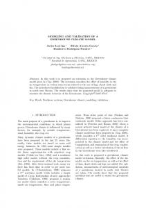
In Figure 4 we show the mean cross-validation accuracy of the support vector machine on 50% training data across 100 random splits. We see that indels alone have much poorer accuracy than SNPs alone and contribute marginally to the SNPs. We achieve a top accuracy of about 82% with the top 20 SNPs. The accuracy drops once we pass the top 20 SNP threshold. Recall that the accuracies shown in Figure 4 are averaged across 100 training validation splits. In each split we first rank the SNPs and compute prediction on validation with top k ranked ones. Thus there is no one set of 20 SNPs to be identified
Cross-validation and cross-study validation of chronic lymphocytic leukaemia
55
here and this is certainly not the same as the top 20 SNPs from the ranking on the full dataset (although there are some in common with top ranked ones from different splits). Alternatively one may consider the intersection of the top 20 SNPs from all 100 split and use them for prediction on an independent external dataset. The drawback there is that not all of the SNPs in the intersection may pass the GATK quality control filtering thresholds. This is why we choose to rank SNPs on the full dataset and consider the first top 100 that are found in the external dataset. Figure 4
Average cross-validation accuracy of support vector machine with top Pearson ranked SNPs and indels together and separately on 100 50:50 training validation splits. Also shown are error bars indicating the standard deviation (see online version for colours)
3.2 Comparison to cross-validation on GWAS To better understand the cross-validation results from SNPs obtained in our whole exome analysis we examine a GWAS for the same subjects. This is an Affymetrix 6.0 genomewide human SNP array of the same disease and subjects that we obtained from the dbGaP site for the whole exome study. We first removed SNPs with more than 10% missing entries and excluded samples that didn’t pass the quality control test with 0.4 threshold in the Affymetrix Genotyping Console. The quality control test measures the differences in contrast distributions for homozygote and heterozygote genotypes in each cel file. Following this we ranked the SNPs with the Pearson correlation coefficient. We then created one hundred random 50:50 train and validation splits and determined the average prediction accuracy of the support vector machine in the same manner as described above for the whole exome study. In Figure 5 we see that the GWAS SNPs give the highest prediction accuracy of 57% in the top 10 SNPs but then it gradually decreases. Thus the SNPs given by our exome analysis which give a higher prediction accuracy may serve as better markers that are not found in the GWAS. Upon closer examination we see that there is no overlap between the top 1000 ranked SNPs from the exome and GWAS datasets except for four that have low Pearson correlation values.
56
A. Aljouie et al.
Figure 5
Average cross-validation accuracy of support vector machine with top Pearson ranked SNPs on 100 50:50 training validation splits of the GWAS dataset (see online version for colours)
3.3 Cross-study validation For cross-study validation on an independent dataset we consider a lymphoma whole exome study that has case subjects for lymphocytic leukaemia as well as a few controls. We also consider controls from a head and neck cancer and a breast cancer study.
Fifteen cases and three controls from a lymphoma whole exome study with dbGaP study ID phs000328.v2.p1 (Pasqualucci et al., 2014). Reads are 101bp length produced from Illumina HiSeq 2000 machine and have 3.4X coverage. The ancestry or origin of data in this study are unavailable in the publication and the dbGaP site.
Three controls from neck and head cancer whole exome study with dbGaP study ID phs000328.v2.p1 (Stransky et al., 2011). Reads are 77bp length produced from Illumina HiSeq 2000 and have 6.9X coverage. Individuals in this study are from the University of Pittsburgh Head and Neck Spore neoplasm virtual repository.
Five controls from breast cancer whole exome study with dbGaP study phs000369.v1.p1 ID (Banerji et al., 2012). Reads are 77bp length produced from Illumina HiSeq 2000 of coverage 5.9X. Individuals in this study have Mexican and Vietnamese ancestry.
In all three datasets we followed a similar procedure that we used for the chronic lymphocytic leukaemia exome dataset. We mapped the short reads to the human genome with the BWA program and detect variants with GATK using the same software and parameters as for the lymphocytic leukaemia dataset. Since this is a validation dataset we cannot use the labels to perform any feature selection or model training. Instead we learn the support vector machine model from the full original dataset. We refer to that as the training set here. We don’t consider all SNPs from the training dataset to build a model. We first obtain the top 1000 Pearson
Cross-validation and cross-study validation of chronic lymphocytic leukaemia
57
correlation coefficient ranked SNPs in the full training. Many of these SNPs don’t pass the GATK quality control tests on some of the external validation samples. One reason for this is the much lower coverage (