Cycle-Based versus Degree-based Classification of Social Networks
Khaled Mahdi1, Maytham Safar2, Ibrahim Sorkhoh3, Ali Kassem4 Chemical Engineering Department College of Engineering & Petroleum Kuwait University P.O. Box 5969 Safat 13060 Kuwait
[email protected]
1
Journal of Digital Information Management
2,3,4 Computer Engineering Department College of Engineering & Petroleum Kuwait University P.O. Box 5969 Safat 13060 Kuwait
[email protected],
[email protected],
[email protected]
ABSTRACT: Complex networks can be classified in three main types: random networks, small-world networks and scale-free networks. Two approaches are tested and compared to identify and classify social networks: one is based on vertex degree and the other on cycle degree. The former approach inaccurately concludes the type of the real network whereas the later accurately identifies the type of the real network. The cycle-based approach reveals Gaussian distribution of the cycles. Cycles distributions of random, small world and scale free networks have one universal Gaussian function. The proposed equation can be used to model, identify and classify any network including social networks. Categories and Subject Descriptors C.2.1 [Network Architecture and Design]: G.1.4 [Quadrature and Numerical Differentiation]; Gaussian quadrature General Terms Network classification, Social networks Keywords Network analysis, Gaussian distribution, Social networks, Received: 18 May 2009; Revised 29 July 2009; Accepted 1 August 2009.
1. Background Networking is the study concerned with analyzing, monitoring, designing or maintaining structures that consist of nodes, links and data transferred through the links to reflect the relationship. Such data is transferred in different formats including and not limited to text, voice, video or signals. One important type of networks is a communication network, for instance phone lines, mobiles, mailing system, e-mails, chatting and the web. In principle, each network has its unique definition of a node, a link and a relationship that dictates the transferred data. One application of networks is the domain of social networks. In social networks, the nodes represent social actors (e.g. Human beings, animals, etc), the links represent the social relationship and the data can take several forms and formats (e.g. text, media, signals, etc). By understanding the characteristics of the links among the actors, we might predict the behavior of the social actor involved; the main motivation of social network studies [9][32].
Journal of Digital Information Management
Social networks analysts have been studying the human sociality [20] for a very long time, and have tried to answer questions: How do people communicate? What are the rules that really control these communications? Half century ago, it was almost impossible to provide qualitative or quantitative assessment to help providing accurate answers to these questions due to lack of statistically sufficient data. Nevertheless, the technological advancement in the communication field and the creation of the Internet and mobiles, the ability to provide insight has grown tremendously. The necessary data surrounding the communications among people can easily be collected from the virtual communities in the Internet, social platforms indifferent to spatial or temporal limitations. Examples of well-known social networks websites of different scope, users and services are Facebook, Hi5, MySpace, LinkedIn and Flicker. Numerous applications of social networks modeling exist in the literature. In [4] they tried to use a mail inbox as a source to develop a social network and asses the network with the objective of fighting spam messages. In [6] they tried to use data stored in banks, phone records, vehicle sales, surveillance reports and registration records to create a social network and to analyze this network to fight criminal organizations. Some other researches tried to use social network to represent web-communities to analyze the World Wide Web. Other applications include data model, compression methods, indexing and query operators were suggested in [1], [3], and [12] respectively to analyze social networks. Most studies characterize social networks using degree distribution, clustering coefficient, average path length and average degree. Recently [10][32] proposed to compute statistical mechanic properties, the cyclic entropy of the network as a measure of the degree of network robustness, such property is based on counting the number of cycles of certain length existing in the network. The research in [8] addressed the problem of correctly relating aliases that belong to the same entity. Their network was constructed from email data mined from the Internet. Links in the network represent web pages on which two email addresses are collocated. The work in [2] analyzed e-mail social network analysis for the detection of security policy violations on computer systems. They assume that the properties of social networks are computationally feasible to evaluate, and in fact can be determined in linear time. In addition, the authors were not able to predict a universal social structure, which can be exploited for encoding all the violations. The study in [11] analyzed a dy-
Volume 7 Number 6
December 2009
383
namic social network in which interactions between individuals are inferred room time-stamped e-mail headers recorded over one year. They discovered that the evolution of such a network is reacted to both the network topology and the application area in which the network is embedded. However, they assumed that global perturbations of such networks are absence, and they used average network properties. Another work in [7] automatically extracted social hierarchies from Enron corporations e-mail data to analyze and catalog patterns of communications between entities to rank relationships. It assumes that the organization is dynamic and its structure changes over time. Almost all the aforementioned research studies analyze networks on the basis of node’s degree. Interestingly, an attempt in [10][15] to characterize social networks by mean of counting cycles and evaluates the network cyclic entropy. However, no comparison to degree-based analysis is based; the purpose of this work. Generally, social networks are classified in three major types: random networks, small-world networks and scale-free networks. These three classes have different topological features. This causes the connectivity between nodes to be different between the three classes. No single unified functional form of degree distribution exists among the major networks types. The main advantage to formulate a unified distribution besides simplifying classification and categorization of networks is to provide a tool to design networks with specific characteristics; such as robustness and prone to failure networks. One challenge in the field of social network is to recognize the real network type correctly and effectively. Current network identification techniques extensively use parameters based on nodes’ degree evaluation mainly: average degree, average length clustering coefficient in addition to the shape of the degree distribution. In section three, we prove the ineffectiveness of degree-based identification techniques. In the subsequent section we provide an alternative identification (or classification) tool. The scope of this work is to study and analyze the three major types of networks and propose a unified formulation of a distribution function of an intrinsic property of the network; cycles in our case. For example, given a real network data, we should be able to recognize the type of social networks by calculating statistical parameters that are unique to a specific type of network. We introduce a new classification based on the cycles existing in the network and compare it to classifications of network based on the degree of the nodes in the network. The aim is to propose a universal form representative distribution of social networks. Our focus is on social networks although it might be applicable to other different types of complex network [21][22][23]. The manuscript is divided into three major parts: the first is the methodology of social network construction adopted by the authors; the second is to classify social networks based on the analysis of node’s degree; the number of links per node; the third is to classify the social networks based on the analysis of the cycles existed in the network. Real network data are obtained from a well-known web friendship application; Hi5.com and Paltalk.
properties that define the model of any complex network, such as the social networks, the connectivity of the nodes in the network and the weights of those connections between the nodes (degree of interaction). The weight is a number that is given to each edge in the network. This number can describe the relation between the two connected vertices in many ways. For example, it could define whether the relation between the two members is tight or strong. In some cases, it might be useful to give the edge only a sign. That is, each relation in the social network is described negatively or positively; for instance hate/love relationship. The second property is the edge nature. Is it directed or undirected? For a social network that the relations on it are usually duplex such brotherhood, it is preferable to represent this relation as an undirected edge. However, sometimes not only the nature of the relation, the application itself enforces the model to be a directed network. We decided to use networks that are undirected and un-weighted because we lack enough information about the relation tightness among the members of the studied social network. We also chose it to be undirected because the generated virtual networks are also undirected as explained in the next subsection. 2.1 Virtual Network Construction The simplest and the most popular network to generate is the random network. With this type of network, connections between each pair of nodes are randomly generated by considering an input design parameter p (probability of connection). Random Network is the simplest model. Its connections are randomly distributed. Because of the lack of a common that gathers a group of actors together, the clustering coefficient for these networks is usually very small. In this network model, it is assumed that there is no such common. The average path length of a random network is usually small and the degree distribution takes the shape of Gaussian Distribution [11]. Generating a virtual network that follows this type is very simple. Considering a probability p that decides the connectivity between the vertices in the network can generate this type of network. Then we can generate the connections between each pairs of the network vertices randomly using p.
The actual and virtual social networks are analyzed subsequently in order to come up with an appropriate model to represent them based on the nature of the data extracted and the application the social network is created for. There are two
Small world is an interesting model that can be found in many real networks. The main property that distinguishes this model from any other is the small world property. This property says that starting from any vertex, any other vertex can be reached by a small number of hubs. The best way to visualize this network is by a set of groups that are strongly connected internally and each group has a small set of connections to another groups. Because of that, this network model has a large clustering coefficient and a small average path length at the same time. There are several real networks that follow this network type. Electric power grids, telephone call networks, neural networks, and many other networks are classified in this model. The degree distribution of this network also takes the shape of Gaussian Distribution [11]. Generating a small world network is a little bit more complicated than random network. The network must be initially a lattice. That is, each vertex has k neighbors. After constructing this initial network, a rewiring probability must be considered. This probability is used to rewire some of the existing edges randomly. To construct small world network, we start by considering all the nodes of the network with no connections between them. Then each node is connected to its nearest k neighbor nodes. After constructing this initial network, a rewiring process is applied, in which each edge in the initial network is rewired randomly based on a probability p. Edge rewiring means, changing the endpoint for an edge from one node to another. In the small-world networks, there are two input design parameters, which are k and p.
384
Volume 7 Number 6
2. Social Network Structure In order to classify the social networks, we need to construct them. In the subsections, we illustrate the construction of virtual random, small word and scale-free networks as explained in details in [11] and the construction of an actual network using an extracted data of virtual friendship network, Paltalk.
Journal of Digital Information Management
December 2009
The World Wide Web network is the most well known network that follows scale-free model. The WWW network has the property of having central hubs. These hubs own the most of the connections in the network. This property is the feature of the scale-free network model. A small number of vertices have a very high degree and most vertices have a very low degree. Other examples of real scale-free networks are: Protein-protein interaction network and the collaboration of actors in films [11]. Scale-free networks are built following a growth pattern. First, the network starts with a random network of size m0. Then the network grows by adding new nodes to the existing network and creating more relations between the newly added node and some of the pre existing nodes. Each time a number of m nodes are added to the existing network. Nodes-adding process ends when reaching the required total number of nodes in the network. However, adding the new relations between a new node i and an existing node v is proportional to the total degree of v. The probability of creating a link between node i and node v is represented by the degree of v over the summation of degrees of all nodes in the network:
p (v ) =
d (v ) , ∑ d (u )
where u ∈ G
(1)
u
where the degree d(v) is the number of neighbors of node v. The larger the degree of v is, the more it is probable for v to get new relations. When creating a scale-free network, two main input design parameters must be specified, m0 and m. Where m0 is the initial randomly created population of nodes with their random set of links and relations. And m is the number of nodes to be added each time to the existing network until reaching the total number of required nodes in the network. In the generation of the virtual network, the selection of the input design parameters is very vital in guaranteeing that the networks generated are as similar as possible to the actual networks. We use a value for p calculated from an actual social network. This probability is calculated by:
p=
2E V ( V − 1)
(2)
where |E| is the number of edges in the network and |V| is the number of vertices in the network. This computes the ratio of the actual number of edges divided by maximum possible number of edges [10]. We chose the rewiring probability as the connection probability of the actual network and the number of neighbors as the average vertex degree of the actual network [10]. Finally, we chose m to be the average vertex degree of the actual network divided by two. The same is assumed and applied to compute m0 [10]. 2.2 Actual Network Construction In addition to the virtually constructed networks, we use data from real social networks such as Hi5 [10] and Paltalk [9]. The first friends network was constructed by extracting a number of records from Hi5 online social network. Hi5 is a social networking website that was founded in 2003 and claims to have over 60 million active members. It is also in the top 10 most visited websites in the world. To construct the friends network, we first created nodes representing each individual and the friends in his list. Then, from a known client, we start extracting the friends of this client then change the current client to the second one in the list as follows:
Journal of Digital Information Management
Create a list and put one client in the list. Pop the first client from the list and make him the current client. If the current client is already processed, don’t extract his friend again. If the current client is not already processed, find his friends and put them in the list and add the current client in the processed clients list. Repeat from step 2 until the desired number of clients is processed. The second real data was extracted from Paltalk; an online chatting program [9] that enables its members to text, voice and video chat with each other in different rooms. Paltalk as a room-based chatting network is more dynamic than other virtual friends network (e.g.,Hi5, Facebook, MySpace). The dynamicity comes from the movement of the members between the rooms. A user can chat with group of users today, and chat with a totally different set of users the next day. Interaction can be between two members or within a large group of members gathered in one chat room. Chat rooms are categorized into different regions or hobbies. For example: Europe, America, Middle East, Sport, Music …etc. Paltalk claims 4 million members worldwide, and on average 50,000 members and 4,000 rooms are online at a time. Members can text chat in more than one room simultaneously, however, they are restricted in accessing a maximum of four rooms at a time. Based on Social network definition, Paltalk is considered as a social network, where its actors are Paltalk’s members and relations are pairs of two members who visited the same room at the same time (i.e. there exists a relation between members x and y if and only if x and y were in the same room at a given time). Moreover the relations between members in this social network are dynamic; since they appear and disappear frequently (i.e. members can visit and leave rooms any time they decide to).
3. Degree-Based Classification The current social network literature [1][8][14][16][21][22][29] emphasizes that any complex network with no specific topology can be classified in one of the three known distinguishable types, Random (RN), Small World (SW), or Scale-Free (SF) using networks properties, all based on nodes’ degree, average vertex degree, clustering coefficient, and average path length [2][10][11]. Average degree ( d ): a vertex degree is the number of the vertices it is connected to. The average vertex degree is an important parameter for characterizing any complex network. The higher the average is, the stronger the vertices are connected to each other. The average vertex degree is calculated by:
d=
1 ∑ d(vi ) N i
(3)
where N is the number of vertices in the network and vi is the ith vertex in the network vertices list [10]. Clustering coefficient: an indication to how much the vertex friends know each other. The network cluster-ability shows how the network members tend to build clusters (a group of members that are strongly related). Calculating the average clustering coefficient (C) is done by using the following formula: C=
1 N
2edges(ne (vi ) (vi ) ne (vi ) − 1
∑ ne i
(4)
where N is the number of vertices in the network, edges(network) is the number of the edges in the network, ne(v) is the vertex
Volume 7 Number 6
December 2009
385
v neighbors sub-network [10]. Average path length (l) is the median of the means of all shortest paths. Calculating this parameter gives a perception of how fast the information can be spread over the network members [10]. On the basis of the above parameters, we should be able to identify and classify any real network and compare it to the parameters of RN, SW or SF distinctively. Such technique we referred to as Network Comparison Technique. In this method, we numerically evaluate the parameters of the actual (real) network and compare them to an equivalent virtual network construct. The other technique is the Network Consistency Technique It considers the real network as being of a specific type and then compute the different network parameters (average vertex degree, clustering coefficient, and average path length) of the real network using analytical equations for well-known network types as suggested in the literatures. Then, we check how close “consistent” those computed values are to the numerically calculated values. Figure 1 illustrates both methods.
Figure 2. Average vertex degree comparison
We calculate the average parameters as shown in Tables 1 and 2, both methods lead to the same conclusion. The actual network is closer to a small world network. However, examining the influence of network size on these parameters, shown in Figures 2, 3 and 4, provide a different insight. The results are misleading and not sufficient to confidently confirm the type of the actual networks based on the calculated parameters. The average vertex degree plot reveals that the actual network can be scale free or small world (both coinciding on the plot). The clustering coefficient plot suggests that the actual network is almost definitely a small world. Whereas, the average path length plot indicates that the actual network can be both random and small world (the RN and SW are coincided in the figure). Unfortunately, we cannot conclude decisively on the type of the actual social network using the major degree-based parameters. This motivates us to search for another intrinsic property of the network that can be effectively used to identify the type of the actual networks; to be discussed in the following section.
Figure 3. Clustering Coefficient
Figure 4. Average Path length Comparison
Network Type
Average Degree
Clustering Coefficient
Average Path Length
Random
2.52
0.03
2.52
Small World
16.57
0.72
NA
Scale-Free
NA
0.01
6.04
Actual Network
16.57
0.65
3.43
Figure 1. Flowchart illustrating the Network comparison and consistency techniques.
Table 1. Network Consistency Technique.NA (Not Applicable) as no analytical expression due to discontinuity in the network
386
Volume 7 Number 6
Journal of Digital Information Management
December 2009
Network Type
Average Degree
Clustering Coefficient
Average Path Length
Random
33.22
0.05
1.96
Small World
16.57
0.67
2.83
Scale-Free
16.17
0.01
6.04
Actual Network
16.57
0.65
3.43
Table 2. Network Comparison Technique
4. Cycle-Based Classification Motivated by the failure of degree-based parameters to decisively identify the real social network type. In addition, there exists no unified form of a distribution function of all major network types since characterization of social network through the degree leads to different non-universal forms of distribution. Random network has a Poisson distribution of the vertices degree. Small-World network has generalized binomial distribution. Scale-Free network has a power law distribution form. There is no universality class reported yet. Here, we propose a universal distribution form that is applicable for all social networks by using the degree of loops or cycles existing in a social network. Consequently, we can identify the type of the real network based on the function parameters. The main question is what intrinsic microscopic property of the network we should use. Social network researchers who use the degree of vertices as an intrinsic property justify their selection from the social question: How many people a social actor in a network is connected to others? By knowing the links a person in a network has, we can derive other topological information based on such information. Another social question that can be asked is how many itineraries the same information dispatched by a given social actor will return to the same person in a social network? It is another way of asking how many cycles existing in the network per person. Closed itinerary, path, loop or cycle, all referred to the same path originates and end in the same node in a graph, the mathematical representation of a network. Cycles exist in none hierarchal networks, most social networks. Such a microscopic property is not widely looked at in social network analysis due to the computational challenges encountered in counting the cycles existing in graph, a known problem in the literature. The authors proved by using cycles as a microscopic property, interesting information could be derived such as the optimal size of a fully connected network, introducing the concept of the form of an ideal social network [13]. In this section, we examine the use of cycles distribution in a network as a method to characterize and classify social network [32]. First, we discuss counting the cycles in a network and next we find the cycles distribution functions of the three major networks as well as the actual network and propose a universal form of the distribution. 4.1 Counting Cycles In order to compute the cyclic entropy of a network, we need to first count the number of existing loops (cycles) in the network. We need to do this counting in the most efficient way. Hence, we modified a well known algorithm in the literature to be used for such a purpose. When counting the loops in a network, multiple loops on the same set of vertices that are in the same direction but with different start vertices will be counted as one loop. However, loops with different directions are considered as different loops. For example, the cycle “X Y Z” is different than “X Z Y”. We are not interested in the members of the cycles; we need only its length. However, we need to save it
Journal of Digital Information Management
in a database to avoid redundancy and multiple counting. Our algorithm is based on the iterative loop counting algorithm (ILCA) [30]. We modified this algorithm to meet our network criteria. ILCA is developed to find all the loops in any connected undirected graph by starting from any vertex or a vertex that has the most links and then search all the paths from it. To determine the cycles distribution, we need to count the number of cycles for each possible cycle length in the network. For this purpose, we utilize a backtracking, described in [7][9]. This Algorithm has a time complexity of O((n+e)c) where n is the number of nodes, e is the number of edges and c is the number of cycles in the network. The algorithm can be summarized in the following steps: 1. Assign IDs for all nodes in the network. 2. Choose node S as the node with least ID. 3. Initialize a path by making S is the root of the path. 4. Start a depth first traversal using S as the root, for each new unblocked node add it to the current path. 5. If S is found again, then a new cycle is found and displayed. 6. When a node is finished, it is set to unblocked so that it can be used in another cycle. 7. After finishing all the nodes, remove S from the network and start again from step 2. 8. If S is the last node in the network, End the algorithm 4.2 Cycles Distribution Function In the experiments we construct networks of the major types using the procedure outlined in Section 2. Networks are generated of different sizes varying from 10 to 25 nodes and different network parameters (p for random networks, p and k for small-world networks and m0 & m for scale free networks). Then, we use the algorithm explained in Section 4.1 to count cycles of different sizes. Consequently, the probability distributions of the cycles existing in the tested networks are determined. In each run, we observe the large number of cycles found in each network, approximately 107 cycles. Hence, Central Limit Theorem (CLT) [26][31] is applicable to the cycle size being random variable. The central limit theorem states that as we increase the size of the sample, the random variables reach a normal distribution. In addition, a plot of the cycles number versus their sizes reveal a bell shape plot, Figures 5-7. For all tested networks, all plots clearly show Gaussian distributions [26][31][32]. The function can be expressed mathematically as:
y ( x) = a e
⎛ x −b ⎞ −⎜ ⎟ ⎝ c ⎠
2
(5)
where a, b and c are positive real numbers. And the parameter a is the y-value of the peak. The parameter b is the x-value of the peak. And the parameter c controls the width of the bell-shape. The function has two inflection points. These points are at x = b - c and x = b + c. The parameters are found through nonlinear regression. Matlab 7.0 is used to perform the regression [27]. We propose this function to represent any given network of any type. This universal representation of networks may help in networks design and characterization. Table 3 summarizes the regression for all types of networks: RN, SW, SF and real network. Figure 5 shows the cycles distribution of a random network with 20 nodes and a connectivity probability p = 0.2. The regression resulted in a = 0.1912, b = 15.9145 and c = 2.9613. Then the graph of the proposed Gaussian function is plotted in the same figure (Figure 5) using the resulting parameters. The same experiment with small-world networks is shown in Figure 6. It shows the cycles distribution of a small-world network with 20 nodes and with parameters p = 0.2 and k = 3. The regression resulted in
Volume 7 Number 6
December 2009
387
a = 0.2182, b = 16.9718 and c = 2.6114. Then the graph of the proposed Gaussian function is plotted in the same figure (Figure 6) using the resulting parameters. Figure 7 shows the cycles distribution of a scale-free network with 20 nodes and with parameters m0 = 3 and m = 3. The regression resulted in a = 0.1756, b = 11.9872 and c = 3.2376. Then the graph of the proposed Gaussian function is plotted in the same figure (Figure 7) using the resulting parameters. Finally, we tested the extracted social network from Paltalk in the same way. The network consists of 26 nodes. The regression resulted in a = 0.1789, b = 18.9995 and c = 3.1583. The cycles distribution of the network and the graph of the proposed Gaussian function are shown in Figure 8. Interestingly, the parameters of the real network are much closer to scale-free network parameters than any other network type. Parameters
X*
Random
N=20 , p=0.2
16 0.190 0.191 15.915
2.961
Smallworld
N=20, p=0.2, k=3
17 0.217 0.218 16.972
2.611
Scale-free
N=20, m0=3, m=3
12 0.173 0.176 11.987
3.238
Actual Network
N=26
19 0.177 0.179
3.158
Network
Y*
a
b
c
Figure 7. Scale-free network with 20 nodes, m0 = 3 and m = 3. The function with a = 0.1756, b = 11.9872 and c = 3.2376
Type
19
Table 3. Regression results of a, b and c of the universal proposed function. X* is the most probable cycle size and Y* is its probability. Note: X* and b are technically the same , they are both network size dependent.
Figure 8. Real social network with 26 nodes. The function with a = 0.1789, b = 18.9995 and c = 3.1583
5. Conclusion
Figure 5. Random network with 20 nodes and p = 0.2. The function with a = 0.1912, b = 15.9145 and c = 2.9613
In attempt to identify and classify a real social network, two approaches are considered, one is based on the evaluation of degree-based parameters and the other is based on evaluating the parameters of cycles distribution. In the first approach, no solid conclusion is derived on the type of real network, whether random, small world or scale free. However, in the second approach, the real network is closer to scale-free than any other type. In addition, the cycles distribution function presents one universal mathematical form. The distinction among different network types is based on the first moment a and the third moment c which distinctively differentiate the networks. Other parameters in the cycle distribution are size dependent and should not be used as benchmarks for different network types.
References [1] Bagchi, A. et al. (2006). Design of a data model for social network applications, Journal of Database Management. [2] Batagelj, V. et al. (2005). Exploratory Social Network Analysis with Pajek (Structural Analysis in the Social Science). Cambridge University Press, England. [3] Bhanu, T. C. et al. (2006). Pre-processing and path normalization of a web graph used as a social network, Journal of Digital Information Management, 4 Figure 6. Small-world network with 20 nodes, p = 0.2 and k = 3. The function with a = 0.2182, b = 16.9718 and c = 2.6114
[4] Boykin, P., Roychowdhury, V. (2005). Leveraging Social Networks to Fight Spam, Computer , 38 (4) 61-68.
388
Volume 7 Number 6
Journal of Digital Information Management
December 2009
[5] Cormen, T. et al (2001). Introduction to Algorithms (2nd ed.). London: The MIT Press.
[19] Safar, M., Ghaith, H.B (2006). Friends Network, In: IADIS International Conference WWW/Internet, Murcia, Spain.
[6] Hsinchun, C., Jennifer, X. (2005). Criminal Network Analysis and Visualization, Communications of ACM, 100-107.
[20] Fiske, A. P. (1998). Human Sociality, International Society for the Study of Personal Relationships Bulletin, v. 14, p. 4-9.
[7] Johnson, D. B. (1975). Finding All the Elementary Circuits of a Directed Graph. SIAM Journal on Computing, 77-84.
[21] Costa, L. d. F., Rodrigues, F. A., Travieso, G., Boas, P. R. V (2007). Characterization of complex networks: A survey of measurements, Advances in Physics, 56, 167 – 242.
[8] Knoke, D., Yang, S. (2008). Social Network Analysis (2nd ed.). SAGE. [9] Mahdi, K. et al. (2008). Temporal Evolution of Social Networks in PaltalkTM. The 10th International Conference on Information Integration and Web-based Applications & Services (iiWAS). [10] Mahdi, K. et al, 2008. Entropy Of Robust Social Networks. The International e-Society Conference. [11] Mahdi, K. et al (2009). A Model of Diffusion Parameter Characterizing Social Networks, In: Proceedings of IADIS International Conference e-Society, 2009. [12] Mitra, S. e. (2006). Complex queries on web graph representing a social network. 1st International Conference on Digital Information Management, (pp. 430-435). Bangalore, India. [13] Safar, M. et al (2008). Maximum Entropy of Fully Connected Social Network. The International Conference on Web Based Communities. [14] Scott, J. (2000). Social Network Analysis: a Handbook. Sage Publications Ltd; Second Edition, U.S.A. [15] Sorkhoh, I. et al (2008). Classification of Social Networks. The International Conference on WWW/Internet. [16] Wasserman, S., Faust, K (1994). Social Network Analysis: Methods and Applications. Cambridge University Press, England. [[17] http://en.wikipedia.org/wiki/Gaussian_function. [18] Shirazi, S. A. J. (2006). Social Networking: Orkut, Facebook, and Gather, In: Blogcritics.
Journal of Digital Information Management
[22] Albert, R., Barabasi, A.-L (2002). Statistical mechanics of complex networks, Reviews of Modern Physics, 74. [23] Albert, R., Jeong, H., Barabasi, A.-L (2000). Error and attack tolerance of complex networks, Nature, 406, 378-382. [24] Wang, B., Tang, H. Guo, C. ,Xiu, Z (2005). Entropy optimization of scale-free networks’ robustness to random failures, Physica A, 363, 591-596. [25] Plischke, M., Bergersen, B (1994) .Equilibrium Statistical Physics, second ed.: World Scientific. [26] Callen, H. B. (1985). Thermodynamics and an Introduction to Thermostatistics, second ed.: Wiley. [27] Kirk, J. (2006). MATLAB Central - File detail - Count Loops in a Graph, MATLAB Central. [28] Agnarsson, G., Greenlaw, R. (2006). Graph Theory: Modeling, Applications, and Algorithms: Pearson/Prentice Hall. [29] Freeman, L. C (2004). The Development of Social Network Analysis: A Study in the Sociology of Science: BookSurge. [30] Mathworks http://www.mathworks.com/matlabcentral/ fileexchange/loadFile.do?objectId=10722&objectType=FILE. [31] Gravetter, F. J., Wallnau, L. B (2008). Statistics for the Behavioral Sciences: Wadsworth Publishing; 8th edition. [32] Safar, M., Mahdi, K., Qassim, A. (2009). Universal Cycles Distribution Function of Social Networks, In: Proceedings of the First International Conference on Networked Digital Technologies’ (NDT).
Volume 7 Number 6
December 2009
389