Damage Detection by Drive-by Monitoring Using the

Damage Detection by Drive-by Monitoring Using the Vertical Displacements of a Bridge D. Martinez School of Civil Engineering, University College Dublin, Ireland

E.J. OBrien School of Civil Engineering, University College Dublin, Ireland

E. Sevillano

School of Civil Engineering, University College Dublin, Ireland ABSTRACT: Drive-by monitoring has received increasing attention in recent years, as it has great potential useful for Structural Health Monitoring (SHM) applications. Although direct instrumentation of civil infrastructures has been demonstrated to be a way of detecting damage, it is also a very expensive method as it requires data acquisition, storage and transmission facilities on each bridge. Drive-by constitutes an alternative that allows the monitoring of a bridge without the necessity of installing sensors on it. In this numerical study, the vertical displacements of the bridge are used for damage detection purposes. The goal of this paper is to describe a model that can reproduce the vertical displacements of the bridge when a simulated vehicle is driving through and show how these displacements change with damage. Vertical displacements are calculated before and after damage, so that the sensitivity of the data to bridge damage can be determined. A finite element (FE) model of a simply supported beam interacting with a moving half car is used in this study. Damage is represented as a loss of stiffness in several parts of the bridge. Vertical displacements are generated at a moving reference for healthy and damaged states, corresponding to vehicle location on the bridge. Two options are explored, the first axle and the second one, as the locations to fix the simulated sensor on the vehicle. Keywords: drive-by, monitoring, bridge, Structural Health Monitoring, SHM, moving reference. 1 INTRODUCTION Damage clearly changes some of the mechanical properties of a bridge such as the frequency (Salawu, 1997), the deflection (Zhu & Law, 2006) and the acceleration (Hester & González, 2012) responses to a given load. First natural frequency tends to decrease when there is damage (Salawu, 1997) whilst deflection increases (Bilello & Bergman, 2004). Nowadays, alternatives to the traditional SHM techniques are needed, given that many of these monitoring methodologies require the installation of complex and expensive sensing and data handling electronics. Such equipment may need to be installed in structures with difficult access and many have safety implications (Keenahan et al., 2013). Some of these issues have prompted a move towards the instrumentation of a vehicle instead of the bridge itself, especially for short span bridges (Kim et al., 2011). Some advantages exist for this concept such as the use of the same vehicle for several bridges and not only for one bridge as in the case in the direct instrumentation. Fewer people are needed to obtain the results and fewer errors are likely as there is no need to install any device. Falling Weight Deflectometer (FWD) is used to measure the stiffness of pavements, but on busy roads it creates traffic problems, as it must be stationary when measuring. The

FWD is a vehicle-mounted device which through its onboard geophones and a weight can determine the stiffness of a pavement. It can also be used to find a bridge’s stiffness, using several loads and averaging these loads and the displacements (Fernstrom et al., 2013). The Traffic Speed Deflectometer (TSD), which was designed to measure pavement stiffness, could be described as a moving equivalent of the FWD. It is therefore an obvious candidate for a drive-by bridge monitoring vehicle. In drive-by monitoring the instrumented vehicle drives over the bridge at a constant speed (González et al., 2012, Malekjafarian et al., 2015). No traffic problems are caused and the data needed can be measured using on board sensors, power and electronics. In many studies, damage detection was attempted using bridge natural frequencies (Salawu, 1997), mode shapes (Malekjafarian & OBrien, 2014) or damping (Keenahan et al., 2013). The properties of the bridge and those of the vehicle have to be defined in order to compare the healthy and damaged situations. Vertical deflections are used in this study due to the simplicity of analysis. The goal is to show how deflection changes through time and space for 1

healthy and damaged bridges and to determine sensitivity to damage. 2. SENSIVITY TO DAMAGE OF THE BRIDGE RESPONSE A potential advantage of drive-by is that the sensors must pass at some time over the damaged parts (Malekjafarian et al., 2015). Vertical displacements vary as the simulated vehicle crosses the bridge, as a function of both time and location. The displacement in the damage case is clearly greater than in the healthy situation, and is related in some way to the damage (Bilello & Bergman, 2004). The simulation has been done with a MATLAB program using a Half-Car model crossing an EulerBernoulli beam. The Half-Car model has just 4 degrees of freedom (DOFs), two for each axle. The DOFs are referred to as the sprung mass bounce displacement, the sprung mass pitch rotation and the two axle hop displacements of the unsprung masses, as it is shown in Figure 1 (McGetrick et al., 2013).

Table 1. Geometrical and mechanical properties of the modelled vehicle Half-Car Property

Value

Weight of the sprung mass, m Unsprung mass axle 1, m Unsprung mass axle 2 , m Length of the vehicle, Axle spacing, D + D Tire 1 stiffness, K , Tire 2 stiffness, K , Damper 1 stiffness, K , Damper 2 stiffness, K , Damper 1 damping, C , Damper 2 damping, C , Centre of gravity distance from axle 1, D Centre of gravity distance from axle 2, D Height of the vehicle h Constant velocity c

18 t 1000 kg 1000 kg 11.25 m 7.6 m 1.75 × 10 N⁄m 3.5 × 10 N⁄m 4 × 10 N⁄m 10 N⁄m 10 Ns⁄m 2 × 10 Ns⁄m 3.8 m 3.8 m 3.76 m 80 km⁄h

The elements considered in the bridge are 1 dimensional beam elements and Bernoulli’s model is assumed for the interaction. The number of elements and the scanning frequency are set to high values in an attempt to increase resolution in the response signal. An approach length of 100 m has chosen to ensure that all degrees of freedom are in equilibrium when the vehicle arrives to the bridge and a high velocity is chosen in order to represent highway conditions.

Table 2. Geometrical and mechanical properties of the modelled bridge

Figure 1. Diagram of the Half-Car model, adapted from (McGetrick et al., 2013). The values of the simulation are in Table 1

Contact is ensured at each time step between the axles and the relevant points on the bridge. A smooth road surface profile has been used for this example. The healthy bridge has the properties listed in table 2. The nature of the damage is specified in table 3. The model was developed in Matlab.

Bridge Property

Value

Number of elements Scanning frequency Length Young’s modulus 2nd moment of area Mass per unit length Damping First natural frequency Length of the approach

200 1000 20 m 3.5 × 10 N⁄m 1.26 m 37500 kg⁄m 3% 4.26 Hz 100 m

Table 3. Properties of the damage Damage Property

Value

Type of damage Quantity of damage Length of damage Centred location of damage

Loss of stiffness ( ) 20% of 2 m (10% of length) 7.5 m from left bearing

2

3. RESULTS AND DISCUSSION

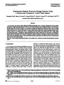
Figure 2. Contour plots of deflection for a) healthy and b) damaged bridges.

The contour plots for the vertical deflection in both the healthy and damaged cases in figure 2. The greatest deflections can be found when the vehicle is close to the mid-span of the bridge. The distributions of the deflections are different for the healthy and damaged cases. With the centre of the damage located at 37.5% of the length of the bridge (7.5 m), the deflection tends to be greater in the first half of the bridge. The moving references of axle location are drawn as diagonal lines in the figure.

Figure 3. Sections through the contour plot at various positions: a) 5m, b) 10 m and c) 15 m.

Damage quantification can be done better than in the constant position situation, due to the smoother graph, as the difference between healthy and damaged situation is progressive, but it is dependent on the location, which is suggested as it was with the constant position figures; for all three figures, deflections are greater around the location of damage.

The flatter parts of the graph at the left and right ends correspond to when there is only one axle on the bridge. It is noteworthy that the slope in the central part of all three graphs gives a slightly indication of damage location.

Figure 5 gives the moving reference cases. The curvature is of interest, these figures reference curvature is generally maximum near the centre but increases locally at the damage region. This follows from the fact that curvature is the ratio of bending moment to stiffness EI. The static bending moment is generally maximum when one of the axles passes the center of the beam. However, there will be a local increase in the damaged region.

The quarter span figure points to the right, the mid span figure points leftwards and the three quarter span figure also points to the left, but with greater slope. The damage severity in indicated by the difference between the healthy and the damaged states, increasing gap suggesting increasing damage. Figure 4 gives sections through the contour plot for given instants in time, as would be captured, for example by a camera based deflection measurement system. 3

4. CONCLUSIONS This paper provides a comparison of three strategies for monitoring the health of a bridge using deflection measurements: fixed in location (point sensor on bridge), fixed in time (snapshot) and moving reference (drive-by). A contour plot provides an overview and cross-sections through that plot show the healthy and damaged responses for each strategy. The drive-by strategy is shown to be competitive with the others and may be particularly promising if curvatures can be extracted. 5. ACKNOWLEDGEMENTS The authors acknowledge the support for the work reported in this paper from the European Union’s Horizon 2020 Research and Innovation Programme under the Marie Sklodowska-Curie grant agreement No. 642453. 6. REFERENCES

Figure 4. Fixed time graphs at a) t= 0.2 s, b) t=0.6 s and c) t=1.0 s.

Figure 5. Bridge displacements at axle location, a) first axle, b) second axle.

BILELLO, C. & BERGMAN, L. A. 2004. Vibration of damaged beams under a moving mass: theory and experimental validation. Journal of Sound and Vibration, 274, 567-582. FERNSTROM, E., CARREIRO, J., RAWN, J. & GRIMMELSMAN, K. 2013. Dynamic Characterization of a Truss Bridge by Falling Weight Deflectometer. Transportation Research Record: Journal of the Transportation Research Board, 2331, 81-89. GONZÁLEZ, A., OBRIEN, E. J. & MCGETRICK, P. J. 2012. Identification of damping in a bridge using a moving instrumented vehicle. Journal of Sound and Vibration, 331, 4115-4131. HESTER, D. & GONZÁLEZ, A. 2012. A wavelet-based damage detection algorithm based on bridge acceleration response to a vehicle. Mechanical Systems and Signal Processing, 28, 145-166. KEENAHAN, J., OBRIEN, E. J., MCGETRICK, P. J. & GONZÁLEZ, A. 2013. The use of a dynamic trucktrailer drive-by system to monitor bridge damping. Structural Health Monitoring, 1475921713513974. KIM, C.-W., ISEMOTO, R., TOSHINAMI, T., KAWATANI, M., MCGETRICK, P. & OBRIEN, E. J. 2011. Experimental investigation of drive-by bridge inspection. 5th International Conference on Structural Health Monitoring of Intelligent Infrastructure (SHMII-5), Cancun, Mexico, 11-15 December,. Instituto de Ingeniería, UNAM. MALEKJAFARIAN, A. & OBRIEN, E. J. 2014. Identification of bridge mode shapes using Short Time Frequency Domain Decomposition of the responses measured in a passing vehicle. Engineering Structures, 81, 386397.

4

MALEKJAFARIAN, A., MCGETRICK, P. J. & OBRIEN, E. J. 2015. A Review of Indirect Bridge Monitoring Using Passing Vehicles. Shock and Vibration, 2015, 16. MCGETRICK, P., KIM, C.-W. & GONZÁLEZ, A. 2013. Dynamic axle force and road profile identification using a moving vehicle. SALAWU, O. S. 1997. Detection of structural damage through changes in frequency: a review. Engineering Structures, 19, 718-723. ZHU, X. Q. & LAW, S. S. 2006. Wavelet-based crack identification of bridge beam from operational deflection time history. International Journal of Solids and Structures, 43, 2299-2317.

5