Structural damage detection using artificial ... - Inderscience Online

Int. J. Sustainable Materials and Structural Systems, Vol. 1, No. 4, 2014

Structural damage detection using artificial neural networks and least square support vector machine with particle swarm harmony search algorithm Ramin Ghiasi and Peyman Torkzadeh* Department of Civil Engineering, Faculty of Technical and Engineering, Shahid Bahonar University of Kerman, Kerman, Iran Fax: +98-341-3220054 Email: [email protected] Email: [email protected] *Corresponding author

Mohammad Noori College of Engineering, California Polytechnic State University at San Luis Obispo, California, USA Email: [email protected] Abstract: The study presented herein compares the performance of structural damage detection using artificial neural networks (ANNs) and least square support vector machines (LS-SMVs). Structural response signals under ambient vibration are processed according to wavelet energy spectrum for feature extraction. The feature vectors are used as inputs to both classifiers based on ANNs and LS-SVMs. LS-SVM parameters along with the selection of input features are optimised using particle swarm harmony search (PSHS) algorithm with a distance evaluation fitness function. The PSHS that has been introduced in this paper is a new hybrid meta-heuristic algorithm for improving the accuracy and the convergence rate of harmony search (HS) algorithm. The effectiveness of different feature extraction methods and different optimisation algorithms are investigated. This investigation shows that although performance of both classifiers is improved by employing PSHS-based selection, for most cases considered, the classification accuracy of LS-SVM is better than ANN. Furthermore, the results demonstrate the efficiency and the robustness of PSHS. Keywords: damage detection; artificial neural networks; ANNs; least square support vector machine; LS-SMV; particle swarm harmony search; PSHS; distance criterion; wavelet packet decomposition. Reference to this paper should be made as follows: Ghiasi, R., Torkzadeh, P. and Noori, M. (2014) ‘Structural damage detection using artificial neural networks and least square support vector machine with particle swarm harmony search algorithm’, Int. J. Sustainable Materials and Structural Systems, Vol. 1, No. 4, pp.303–320.

Copyright © 2014 Inderscience Enterprises Ltd.

303

304

R. Ghiasi et al. Biographical notes: Ramin Ghiasi received his MSc from Department of Civil Engineering in Shahid Bahonar University of Kerman in Iran. His research interests are structural health monitoring, artificial intelligence, metaheuristic optimisation techniques and applications. Peyman Torkzadeh is an Assistant Professor of Department of Civil Engineering in Shahid Bahonar University of Kerman in Iran. He has over 50 papers in various journals and conferences. His research has been in structural health monitoring, structural damage detection, structural optimisation, numerical modelling and seismic design of structures. Mohammad Noori’s research over the last 30 years has been in nonlinear random vibrations and hysteresis, smart materials, seismic isolation and diagnostic methods in structural health monitoring. He was the RJ Reynolds Professor and Head of Mechanical and Aerospace at NC State and the Dean of Engineering at Cal Poly, where he is currently a Professor of Mechanical Engineering. He also has research affiliations with Southeast University in China. He is an ASME Fellow, has published over 200 refereed and technical papers, serves as the executive editor, associate editor and the editorial board member of seven journals.

1

Introduction

Damages in structural systems are generally caused due to dynamic excitations, fatigue, impact and cyclic loadings, temperature variations, corrosion, natural hazards, and/or extreme loading conditions. As the analytical, experimental, and field test results have shown, the incurred damage in a structure leads to a change in the structural dynamic characteristics, such as stiffness, natural frequencies, damping and subsequently dynamic response. The damage identification techniques quantify the conditions of a structure by examining these changes. The core of these methods is to seek some damage indices that are sensitive to structural damage. Doebling et al. (1998) presented a literature review on the damage assessment methodologies based on parameters such as the natural frequencies, mode shapes, mode shape curvature, flexibility matrix and stiffness matrix. Considering a change in the dynamic characteristics, as a measure for detecting the damage, the feasibility of applying artificial intelligence (AI) was considered in order to detect the structural damages (Yan et al., 2014). Liu et al. (2011) presented a structural damage diagnosis method based on combining the wavelet packet decomposition and artificial neural network (ANN) pattern classification. Fan and Liu (2008) employed support vector machine (SVM) and relative change value index of modal flexibility. They concluded this combined method had a good damage detection capability within a certain noise level. A study was performed by Saeed et al. (2011) to identify the cracks in curvilinear beams by using ANN and adaptive neural fuzzy inference system (ANFIS). The results demonstrated that the average prediction errors in the multiple ANN models is less than those in the single ANN model and multiple ANFIS. Saadat et al. (2004) proposed an intelligent parameter varying (IPV) method for damage detection in a highly nonlinear hysteretic system. IPV uses embedded radial basis function (RBF) networks to estimate the constitutive characteristics of inelastic and hysteretic restoring forces in a multi-degree-of-freedom structure. Their results demonstrated the effectiveness of IPV in

Structural damage detection using ANNs and LS-SMV

305

identifying highly nonlinear restoring forces, without a priori information, while preserving a direct association with the structural dynamics. Among the aforementioned methods, SVM is a supervised learning method, which is used for classification and regression with a high accuracy and relatively broad application capability. However, in some cases of structural health monitoring diagnosis, the collected data from the structure may be from a single sensor. Given the accuracy of the collected data from a single source depends on the efficiency and performance of the sensor, as well as the level of the environmental noise, only limited information about the structure’s dynamic response can be collected and the relevant information from the vibration signals may be incomplete, inconsistent or even imprecise. Signals from additional sensors positioned in other locations may provide complementary data in addition to the redundant information content (Guo, 2006). However, if data collected from all sensors are used as input for a classifier, it may result in slow convergence of the classification process and the classification performance can be deteriorated. There are several methods to overcome these problems some of which include; independent component analysis (ICA), and distance criterion feature selection and principal component analysis (PCA) method (Zhong et al., 2006). A few investigators have recently employed genetic algorithm for feature selection and have demonstrated if certain specific features are selected from the utilised diagnostic systems, they can perform better than the original general diagnosis tool (Nguyen et al., 2008; Samanta, 2004). The data transformation to a lower dimension of ICA and PCA techniques is effective, however, there is no guarantee that the removed information is not essential for the damage classification. In specific cases, the feature selection that selects part of the original data can provide better results. In this study, we propose an integrated system consisting of an LS-SVM classifier, which has the ability to select optimal parameters and features, along with a particle swarm harmony search (PSHS) algorithm used in conjunction with that. PSHS is a new hybrid meta-heuristic algorithm that is introduced in this paper, for improving the accuracy and converges rate of HS algorithm. PSHS algorithm is used for not only selecting the features and all LS-SVM parameters, but it is also applied as a distance evaluation technique for the fitness function. For this purpose, Wavelet packet decomposition is applied to the structural response signals under ambient vibration, and feature vectors are obtained via a feature extraction based on wavelet energy spectrum. Subsequently, the best feature vector is selected by the PSHS algorithm and in the final step this selected feature is employed for training the LS-SVM algorithm. Various levels of structural damage detection including the occurrence, location and severity of the damages are studied through a numerical analysis. In order to demonstrate the accuracy of classification by the proposed algorithm, the same system is analysed by an ANN approach and eventually a comparison is made between the performance of both algorithms, with and without automatic selection of features and classifier parameters. Furthermore, the efficacy of using HS or PSO algorithm instead of PSHS, and utilising the statistical characteristics of vibration signals, instead of wavelet packet transform (WPT), is investigated. This paper is organised as follows: in Section 2, we describe the intelligent classification algorithm utilising LS-SVM and ANN. Optimisation algorithm including PSO, HS and the procedure for constructing the PSHS algorithm are represented in Section 3. Feature extracting method utilising WPT and statistical characteristics of

306

R. Ghiasi et al.

dynamic signals are described in Section 4. Damage detection procedure is described in Section 5. Numerical examples are studied in Section 6 and conclusions are presented in Section 7.

2

Intelligent classification algorithms

2.1 Least square support vector machine (LS-SVM) There are various types of SVMs, as a new learning system, based on statistical learning theory. Among these types, LS-SVM with the advantages of simpler algorithm and faster operation speed has been widely applied in pattern recognition and nonlinear regression (Suykens et al., 2002). The regression principle of LS-SVM can be explained as follows. Consider a sample set {(x, y), X ∈ Rn×m, Y ∈ R} and input sample matrix X = [x1; x2; …; xn], in which xi is m dimensional and Y = [y1; y2; …; yn] denotes the output sample column vector. For the regression problem, LS-SVM regression model in the primal weight space can be considered as the following form: y ( x) = ωT φ( x) + b

(1)

The optimisation problem of the above model can be formulated as follows: 1 1 || ω ||2 + γ || ξ ||2 2 2 S.t. φ( x)ω + eb + ξ = Y Min

(2)

where φ(.): Rn → Rnh is the mapping to the high dimensional and potentially infinite dimensional feature space. The parameter γ > 0 denotes a real constant used to control the punishment degree for misclassification and e denotes a column vector with elements equal to 1. Because ω becomes infinite dimensional, this problem cannot directly be solved. Therefore, let us proceed by constructing the following Lagrangian: L(ω, b, ξ , α ) =

1 1 || ω ||2 + γ || ξ ||2 −α T ( φ( x)ω + eb + ξ − Y ) 2 2

(3)

where α is Lagrange multiplier. The conditions for optimality are given by: ∂L ∂L ∂L ∂L = 0, = 0, = 0, =0 ∂ω ∂b ∂ξ ∂α

(4)

After elimination of the variables ω and ξ, a linear Karush-Kuhn-Tucher (KKT) system with a set of n + 1 dimensional linear equations can be obtained: eT ⎤ ⎡ b ⎤ ⎡ 0 ⎤ ⎡0 ⎢ ⎥=⎢ ⎥=⎢ ⎥ ⎣ e K + I / γ ⎦ ⎣α ⎦ ⎣Y ⎦

(5)

where I ∈ Rn×n denotes a unit matrix, α = [α1; α2; …; αN] and K = K(X, X) = φ(x)φ(xT) is a kernel matrix.


307

By solving equation (5), the results of LS-SVM regression model become: y ( x) = K ( X , X )α + b

(6)

2.2 RBF neural network RBF network is a type of feed forward neural networks that learns using a supervised training technique. Lowe and Broomhead (1988) were the first researchers that exploited the use of RBF in design of neural networks. Radial functions are a special class of functions and their characteristics are that response decreases, or increases, monotonically with the distance from a centre point. It has been shown that RBF networks are able to approximate any reasonable continuous function mapping with a satisfactory level of accuracy (Park and Sandberg, 1991). The main difference between ANNs and SVM is in the principle of risk minimisation (RM). In SVM, structural risk minimisation (SRM) principle is used for minimising an upper bound on the expected risk whereas in ANNs, traditional empirical risk minimisation (ERM) is used for minimising the error on the training data. The difference in RM is to improve the general application of SVM compared to ANNs (He and Yan, 2007). In this study, damage detection capability of LS-SVM is compared with that of RBF neural network.

3

Meta-heuristic optimisation algorithms

3.1 Particle swarm optimisation Particle swarm optimisation (PSO) is a swarm based intelligence algorithm, influenced by the social behaviour of animals such as a flock of birds finding a food source or a school of fish protecting themselves from a predator (Eberhart and Kennedy 1995). A particle in PSO is analogous to a bird flying or fish swimming through a search (problem) space. The movement of each particle is coordinated by a velocity which has both magnitude and direction. Each particle’s position at any instance of time is influenced by its best position and the position of the best particle in a problem space. The performance of a particle is measured by a fitness value, which is problem specific. The PSO algorithm is similar to other evolutionary algorithms. In PSO, the population is the number of particles in a problem space. Particles are initialised randomly. Each particle will have a fitness value, which would be evaluated by a fitness function to be optimised in each generation. Each particle knows its best position pbest and the best position so far among the entire group of particles gbest. The pbest of a particle is the best result (fitness value) so far reached by the particle, whereas gbest is the best particle in terms of fitness in an entire population. The particle would have velocity, which directs the flying of the particle. In each generation the velocity and the position of particles are updated as follows: vik +1 = wvik + c1rand1 × ( pbesti − xik ) + c2 rand 2 × ( gbest − xik ) xik +1 = xik + vik +1

(7)

308

R. Ghiasi et al.

where vik

velocity of particle i at iteration k

vik +1

velocity of particle i at iteration k +1

w

inertia weight

ci

acceleration coefficients; j = 1, 2

randi random number between 0 and 1; i = 1, 2

xik

current position of particle i at iteration k

pbesti best position of particle i gbest position of best particle in a population xik +1 position of the particle i at iteration k + 1.

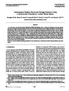
3.2 Harmony search algorithm Harmony search (HS) algorithm is based on natural musical performance processes that occur when a musician searches for a better state of harmony, such as during jazz improvisation. The engineers seek for a global solution which is determined by an objective function, just like the musicians seeking to find musically pleasing harmony as determined by an aesthetic (Geem et al., 2001). Figure 1 shows the optimisation procedure of HS algorithm, which consists of following steps: Step 1

Initialise the algorithm parameters and optimisation operators. HS algorithm includes a number of optimisation operators, such as harmony memory (HM), harmony memory size (HMS), harmony memory considering rate (HMCR) and pitch adjusting rate (PAR). In HS algorithm, HM stores the feasible vectors, which all of them are in the feasible space. The HMS determines the number of vectors to be stored.

Step 2

Improvise a new harmony from HM. A new harmony vector is generated from the HM, based on memory considerations, pitch adjustments and randomisation. Variation of HMCR between 0 and 1 sets the rate of choosing a value in the new vector from the historic values stored in the HM, and (1-HMCR) sets the rate of randomly choosing one value from the possible range of values. The pitch adjusting process is performed only after a value is chosen from the HM. The value (1-PAR) sets the rate of doing nothing. For example, PAR = 0.1 indicates that the algorithm will choose a neighbouring value with 10% × HMCR probability.

Step 3

Update HM. If new harmony vector is better than the worst harmony in the HM, judged in terms of the objective function value, the new harmony is included in the HM and the existing worst harmony is excluded from the HM.

Step 4

Repeat Steps 2 and 3 until terminating criterion is satisfied; otherwise, Steps 2 and 3 are repeated.

Structural damage detection using ANNs and LS-SMV Figure1

309

The flow chart for HS

3.3 The realisation of PSHS based on HS This section describes the implementation of proposed improvement in HS using PSO approach. The proposed method, called PSHS is based on the characteristics of both PSO and HS algorithms. PHSH applies PSO to perform global exploration and HS to perform local search on the solutions produced in the global exploration process. Based on the previous section, at the beginning of the HS algorithm HM matrix is created and filled with randomly generated solutions vectors. It is obvious that if HS is filled by optimised solution vectors, convergence rate of HS is improved. In other words, in the process of HS algorithm the initial random solution vector is improvised until stopping criterion is satisfied. If this initial solution is near the global solution, the process of finding best solution will be faster. Therefore, in hybrid algorithm PSO is substituted with random selection of harmony vector and is used to explore the potential solution space. In summary, process of PSHS can be described as follows: Step 1

Initialising the parameters of PSO and HS.

Step 2

Executing PSO by 20 particles and the global best position after a few iterations have been repeated HMS/2 times in the HM matrix. Remaining part of HM matrix is filled by random solution vectors (harmonies).

Step 3

Performing HS and generating a new solution.

Step 4

If the new solution is better than the worst harmony vector then it replaces that with the new one.

Step 5

The programme is completed if the termination conditions are met otherwise process goes back to Step 3.

In the process of searching for the optimal solution, two fundamental principles should be considered simultaneously. First, the global optimum can be located anywhere in the search space. The second, probability of finding the new solution, that can improve the objective function value, is higher in the vicinity of a solution with a higher objective

310

R. Ghiasi et al.

function value (Randy and Sue, 2004). The PSHS algorithm presented herein employs the two aforementioned strategies simultaneously and effectively together in order to find the optimal solution. By selecting several members of HM by randomisation, using the first strategy, and by replicating the best solution of PSO in HM strategies, the second strategy.

4

Feature extraction methods

4.1 Wavelet packet transform The WPT of a time domain signal f(t) can be calculated using a recursive filter-decimation operation (Coifman and Wickerhauser, 1992). After j-levels of decomposition, the original signal f(t) can be expressed as: 2j

∑f

f (t ) =

i j (t )

(8)

i =1

2j

f ji (t ) =

∑ C (t )ψ i j

i j , k (t )

(9)

i =1

Herein, the component signal f ji (t ) can be expressed by a linear combination of wavelet functions ψ ij , k (t ). Integers i, j and k are the modulation, scale and translation parameters, respectively; C ij (t ) and ψ ij , k (t ) are defined as the wavelet packet coefficient and the wavelet packet function. The wavelet packet coefficients can be obtained from

∫

C ij , k =

∞

−∞

f (t )ψ ij ,k (t )dt

(10)

For the purpose of structural damage detection, frequency domain information tends to be more important and thus a high level of the WPT is often required to detect the sudden changes in the signals. Once the WPT is carried out, the energies of these decomposed component signals can be utilised for structural condition assessment. These component energies are defined as E ij =

∫

∞

−∞

f ji (t ) 2 dt

(11)

It can be shown that, when the mother wavelet is semi-orthogonal or orthogonal (Han et al., 2005), the signal energy Ef is the summation of the j-level component energies as follows: Ef =

∫

∞

−∞

2j

f (t )dt = 2

∑E

i j

(12)

i =1

Generally, we use relative energy to indicate the damage feature, thus, the relative energy Ei in i-frequency band can be expressed as


Ei =

311

E ij

(13)

Ef

4.2 Statistical features (SF) Time-domain vibrational signals from sensors can be preprocessed by the function presented in Table 1 to form the features vector. The features are: root mean square (RMS), variance, skewness, kurtosis, crest factor and the maximum frequency signal at each sensor. These features represent the energy, the vibration amplitude and the time series distribution of the signal in time-domain. Table 1

Time-domain features

Feature Root mean square

Function

rms =

∑

var = σ 2 =

∑

Skewness

skewness =

∑

Kurtosis

kurtosis =

∑

Maximum value

5

( x( n) )

2

N

Variance

Crest factor

N n =1

N n =1

( x(n) − mean( x) )

2

( N − 1) N n =1

3

( N − 1)σ 3

N n =1

crest =

( x(n) − mean( x) )

( x(n) − mean( x) )

4

( N − 1)σ 4 max x( n) rms

max = max|x(n)|

Damage detection procedure

5.1 Extracting data and creating input vector A data fusion technique can combine data from several information sources, as well as the information from the relative data-bases, to achieve a higher accuracy and more specific inferences than what could be achieved by a single source alone (Telmoudi and Chakhar, 2004). Feature fusion is one kind of data fusion; it integrates information from different sensors and obtains feature vectors (Chen and Jen, 2000). Since the LS-SVM is very suitable for feature fusion detection, a damage detection method based on feature fusion and LS-SVM model is herein proposed.

R. Ghiasi et al.

312 A

When using WPT as data extraction method: 1 Battle-Lemarie wavelet is symmetric, the wavelet function is a band filter in the frequency domain, while the scale function is a low-pass filter. Thus, frequency bands of the above two functions are overlapped in certain degree. This shows a favourable orthogonal characteristic (Mallat, 1989). In order to decompose the signals to be analysed into different frequency bands and make each frequency band energy independent and irredundant, Battle-Lemarie is adopted as the basis wavelet package function in this paper. Several optional measuring nodes are selected, and vibration signals from these nodes are analysed by using the WPT first. 2 The level of wavelet packet decomposition is determined through a trial and error sensitivity analysis using both the healthy and the damaged structural models. The frequency band energy is then calculated and normalised. The wavelet package relative energy (WPRE) of the signals from sensor s is E ps = { Em , m = 1, ..., M }

(14)

where s = 1, 2, …, S, p is the acquiring number, p = 1, 2, 3, …, P. 3

The WPRE E ps of the signals from sensor s is combined to obtain the fused feature vector E p = { E1p , E p2 , ..., E ps }

4

B

(15)

A well trained LS-SVM, with the structural damage fused feature proxy Ep, as the inputs, and the corresponding damage condition, as the outputs, is applied to classify and identify the samples based on the given principles. The damage assessment results are therefore, obtained.

When using statistical features as data extraction method: Time-domain vibrational signals from sensors are preprocessed by equations given in Table 1 to form the feature training and test sets. Each feature is normalised by dividing it by the maximum of its absolute value before using that for training and testing the LS-SVM models.

5.2 Creating harmony vector In this study, LS-SVM and RBF neural network are employed for damage detection. PSHS algorithm is designed for the feature selection and the LS-SVM parameter optimisation. For this purpose, harmony vector has been formatted in a binary form in such a way that the first 6 × i data in this vector represent features of vibrational signal of the i sensor. By this procedure, the value of ‘1’ means the feature is selected and the value of ‘0’ indicates that the feature is not selected. Next two data in harmony vector represent C and σ2 parameters of LS-SVM. C is the regularisation parameter that determines a trade-off between the training error minimisation and the smoothness. Parameter σ2 is the squared bandwidth of Gaussian RBF kernel. These parameters change continuously between the predefined upper and lower bounds.


313

5.3 Fitness function Fitness function is an important factor for the speed and the efficiency of PSHS algorithm. In this study, the fitness function of HS is developed based on LS-SVM training accuracy and the number of selected features. The LS-SVM accuracy is obtained by the evaluation of the test data classification using the trained model. By using this fitness function, the LS-SVM parameters are optimised and the number of features are also selected. PSHS selects the vector with the smallest fitness value after the termination conditions are satisfied. The fitness function of PSHS is formed as follows (Nguyen et al., 2008): F = W × ( LS − SVM trainingaccuracy ) + (1 − W ) −1

×

∑ ∑

classes

classes

within − class distance

(16)

between − class distance

Equation (16) can be rewritten as: F = W × ( LS − SVM trainingaccuracy ) + (1 − W ) × −1

Jc Jb

(17)

where W is weighting factor with the value between 0 to 1. The within-class distance is given by: c

Jc =

∑pJ

(18)

i i

i =1

n

T ⎛1⎞ J i = ⎜ ⎟ ( xki − mi ) ( xki − mi ) ⎝ ni ⎠ k =1

∑

(19)

where class i = 1, …, c; mi is the mean vector of class i; ni is the number of samples in class i and pi is the ratio factor between the number of samples in class i and the total samples. The between-class distance is: c

Jb =

∑ p (m − m)

T

i

i

( mi − m )

(20)

k =1

where m is the mean vector of all classes. In this study, class means the damage pattern. The ratio Jc/Jb is used to obtain the optimal features based on the criterion that chooses the smaller within-class distance Jc and the larger between-class distance Jb. The number of features is selected based on minimising Jc/Jb ratio.

5.4 Block diagram Figure 2 presents a block diagram of PSHS programme that is used to look for an optimal feature subset and LS-SVM parameters. When the termination condition is satisfied, the best member is obtained and used to receive the needed information.

R. Ghiasi et al.

314 Figure 2

6

The flow chart of the system

Damage detection example

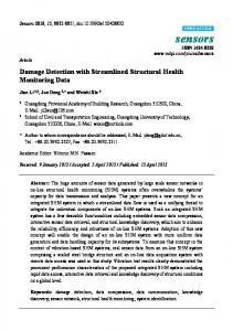
The four-story steel structure shown in Figure 3 has 12 degrees of freedom (DOF). This structure has a base plan of 2.5 m × 2.5 m and a height of 3.6 m. The quarter-scale symmetrical model of structure was developed and studied in the Earthquake Engineering Research Laboratory at the University of British Columbia (UBC) (Johnson et al., 2003). The members are hot rolled grade 300 W steel with a nominal yield stress of 300 MPa (42.6 kpsi). The excitation is a low-level ambient wind loading at each floor in y-direction. To consider the uncertainty of environmental loads, the wind loading is modelled as a filtered Gaussian white noise process passed through a sixth order low-pass Butterworth filter with a 100 Hz cut-off. Sensors are installed in each floor on the side end middle column; there are in total 16 sensors. Signals to be analysed are the


315

acceleration response signals gathered from each floor sensors. The sampling frequency is 100 Hz; the length of the data is 40,000. Figure 3

Four-story structure of ASCE health monitoring benchmark studies, (a) schematic drawing (b) node numbering in finite element model

(a)

(b)

316

R. Ghiasi et al.

6.1 Extracted features Battle-Lemarie as a basis function is employed to decompose the acceleration responses with 4 as the decomposition level. 16 frequency bands in total are generated, the width of which is 3.91 Hz. These component energies are sorted first according to their magnitude, 95% of the WPRE is mainly distributed below 100 Hz frequency bands after calculation, which are both significant in value and sensitive to the damage of the structure. Therefore, the first 6 component energies of WPT are selected as damage indices. In statistical features case, by preprocessing of vibrational signal of each sensor we have 6 features per sensor. Thus, we have a total of 96 features for each damage scenario for each method of data extraction.

6.2 Damage occurrence and damage location For damage detection by the proposed algorithm we incorporate the damages by removing the braces in y-direction. Relative calculation indicates that the damage of beams and the braces in x-direction has low effects on the vibrational responses. Therefore, only the damage of braces in y-direction is investigated in this study. Damage severity is described by removing four braces, three braces, two braces and one brace, respectively. Furthermore, it is assumed that damages occur in one, two, three and all four floors of the structure. For example, when damage is restricted to one floor, we have 4 × 4 damage scenarios. Therefore, all damage scenarios include: 1

Damages in one floor: 4 × 4 = 16

2

Damages in two floors: 4 × 6 = 24

3

Damages in three floors: 4 × 4 = 16

4

Damages in four floors: 4 × 1 = 4.

With the above damages, in addition to the case of no damage, there are in total 61 damaged cases. Considering the effect of the environmental noise, random Gaussian white noise with different severity is added to the acceleration responses of the above 61 damage cases. The ratios of the maximum RMS values between the noise and the signal for the 61 cases are 10%, 20% and 30%, respectively. These are named as the samples I to III. Samples I and II are used as training samples and sample III are employed for testing. Therefore, 183 samples are used in simulation of damage identification, including 61 testing samples and 122 training samples. Signals are preprocessed similar to what described in the previous section, then the best feature is selected by PSHS algorithm. The kernel functions of LS-SVM are the RBF functions. The PSHS parameters are: number of iterations for HS = 5,000, HMS = 40, HMCR = 0.9, PAR = 0.5, number of particles = 20, and c1 = c2 = 0.8. The value of inertia weight in velocity formula of PSO decreases linearly from 0.9 in the first iteration to 0.4 in the 1000th iteration of PSO. The weighting factor W in fitness function is varied from 0.6 to 0.9 to get the different sets of features. All 96 features of each damaged case are the input of both algorithms. The output numerical value is the damaged case as


317

previously mentioned in this study; we have 61 damage cases. Number of neurons for RBF neural networks is equal to the number of inputs. Table 2 shows the effect of selecting WPT or statistical features as data extraction methods on the damage detection accuracy of classification algorithms. Ratio of correctly detected damage cases to all test data (61 cases) is defined as damage detection accuracy (DDA). The result show that the accuracy of damage detection based on WPT is higher than that based on statistical features under the same conditions. This is due to the fact that WPT is a powerful mathematical tool for capturing changes of structural characteristics/properties induced by damage. As compared with statistical features, WPT provides an effective feature extraction procedure for compressing the data measured and obtaining useful information for damage assessment. In other words, the features that are acquired by WPT from vibrational signal have higher sensitivity to the damage of the structure in comparison with the features that are acquired by statistical features. Therefore, we use WPT as the data extraction method for other studies in this paper. Table 2

Comparing the performance of data extraction methods RBFNN

LS-SVM

Input feature

DDA (%)

Training time (s)

DDA (%)

Training time (s)

Statistical feature

All

83.12%

28

81.1%

22

Wavelet pocket transform

All

91%

31

87%

27

Dataset

Table 3 shows the DDA for classification methods with PSHS algorithm compared by other meta-heuristic optimisation algorithms. Results demonstrate the efficiency and robustness of PHSH, which performs better than PSO and HS. This is due to the fact that, PSHS combines the advantages of both algorithms and PSO helps HS process not only to efficiently perform the global exploration for rapidly attaining the feasible solution space, but also effectively helps to reach optimal or near optimal solution. Table 3

Optimiser algorithm

Comparing the performance of optimisation algorithms RBFNN

LS-SVM Par. LS-SVM σ2, C

DDA (%)

10, 23, 56, 76, 77, 79, 80

1.25–3.47

98.68%

97.66%

5, 10, 17, 31, 41, 53, 79, 84, 94

1.092–2.01

98.2%

99%

11, 16, 32, 60, 80

1.62–2.23

100%

Input features

DDA (%)

Input features

PSO

10, 26, 33, 49, 72, 79, 84, 94

98%

Harmony

12, 33, 37, 79, 80

PSHS

11, 15, 20, 35, 60, 80

Table 4 and Table 5 show the results of damage location and damage severity by using PSHS selection with LS-SVM and RBF neural network, respectively. In Table 4 and Table 5, the selection with a few number of features and the larger accuracy can be chosen from DDA and the features set. For LS-SVM with RBF kernel in Table 4, the feature set: 11, 16, 32, 60 and 80 is the best choice. This set has only five features and gives the highest performance compared with others. These features have

318

R. Ghiasi et al.

been selected from 96 available features. In Table 5, when RBF neural network is used, the set: 11, 15, 20, 60 and 80 can be the best choice. It has the small number of features (6 features) and a higher performance. Furthermore, features 11, 60 and 80 are common in both the best feature set, hence, the selection of this feature has a high performance in damage detection procedure. Table 4

Test of damage location and damage severity using PSHS algorithm and LS-SVM Parameter σ2

Parameter C

DDA (%)

5, 10, 11, 16, 17, 22, 28, 31, 41, 53, 60, 72, 79, 84, 94

1.4301

2.4393

98%

10, 76, 77, 79, 80

2.2558

1.0504

96%

11, 16, 32, 60, 80

1.6261

2.2372

100%

28, 32, 52, 80

1.3818

1.4404

96%

Selected feature

Table 5

Test of damage location and damage severity using PSHS algorithm and RBF neural network

Selected feature

DDA (%)

10, 26, 33, 49, 72, 79, 84, 94

85%

12, 33, 37, 79, 80

95%

11, 15, 20, 35, 60, 80

99%

13, 32, 54, 91

90%

In order to confirm the efficiency of the proposed selections, the performances of LS-SVM and RBF neural networks for the selected feature subsets and all features are obtained and the results are shown in Table 6. When all the features are considered, the procedure is repeated 100 times with random parameters to get the average results. The LS-SVM parameters are randomly chosen in the range of 0 to 50. The results represent that the efficiency of the proposed selections for reducing the number of features and also determining the LS-SVM parameters is suitable. Table 6 shows that the damage detection accuracy is increased by using the PSHS algorithm, while the number of features is significantly decreased. In LS-SVM case, the accuracy is increased from 87% to 100% with 94.8% data reduction. In case of RBF neural network, the accuracy is increased to 99% with 93.75% data reduction. Generally, Table 6 shows that LS-SVM has a high accuracy and performance for damage detection of the structure with and without PSHS selection. In addition, performance of RBF neural network is increased with PSHS selection but damage detection accuracy of LS-SVM is better than RBF neural network. Table 6

Comparing the performance of proposed LS-SVM and RBF neural network for selected features and all features

Algorithm

Feature

Parameter σ2

Parameter C

DDA (%)

LS-SVM

All

1.5

2.5

87%

RBF network LS-SVM RBF network

All

-

-

91%

11, 16, 32, 60, 80

1.6261

2.2372

100%

11, 15, 20, 35, 60, 80

-

-

99%


7

319

Results and discussion

In this study, a method was presented for structural damage detection using two classifiers, namely, RBF neural networks and LS-SVM with PSHS-based feature selection from time-domain vibration signals. The selection of the input features and the appropriate classifier parameters have been optimised by using PSHS-based approach. The roles of different feature extraction methods, WPT and statistical feature, and different optimisation algorithms, HS, PSO and PSHS, were investigated. In order to assess the performance of the proposed method for structural damage detection, benchmark dataset from IASC-ASCE SHM group was considered. Based on the numerical results, the following conclusions resulted: 1

Selecting the parameters and training the inputs for LS-SVM have high influence on the system performance. The feature selection can remove the irrelevant and the redundant information by choosing useful features as input of LS-SVM, while each proper parameter helps to build the high performance and accuracy of LS-SVM model.

2

Although performance of both classifiers is improved by using PSHS-based selection, for most cases considered, the classification accuracy by LS-SVM is better than that of RBF neural network. The use of PSHS with only few features provide 100% classification accuracy for LS-SVM.

3

The results show that the potential application of PSHS algorithm for selection of features and classifier parameters for damage detection.

4

The combination of the WPT, feature selection by PSHS and LS-SVM model, is suitable for the structural damage detection. This method can also correctly identify the location and the severity of damages in the structure.

5

Wavelet transform has emerged as a powerful mathematical tool for capturing changes of structural characteristics/properties induced by damage. It provides an effective feature extraction procedure for compressing the data measured and obtaining useful information for damage assessment. The WPT-based component energies extracted appear to be good indicators that can reveal the health condition of structures.

6

PHSH algorithm presented in this paper is a special combination of PSO and harmony algorithms, and compared with them has a higher convergence rate and requires less computational time and effort.

References Chen, S-L. and Jen, Y.W. (2000) ‘Data fusion neural network for tool condition monitoring in CNC milling machining’, International Journal of Machine Tools and Manufacture, Vol. 40, No. 3, pp.381–400. Coifman, R.R. and Wickerhauser, M.V. (1992) ‘Entropy-based algorithms for best basis selection’, IEEE Transactions on Information Theory, Vol. 38, No. 2, pp.713–718. Doebling, S.W., Farrar, C.R. and Prime, M.B. (1998) ‘A summary review of vibration-based damage identification methods’, Shock and Vibration Digest, Vol. 30, No. 2, pp.91–105.

320

R. Ghiasi et al.

Eberhart, R. and Kennedy, J. (1995) ‘A new optimizer using particle swarm theory’, in Proceedings of the Sixth International Symposium on Micro Machine and Human Science, MHS’95, IEEE, pp.39–43. Fan, X. and Liu, T. (2008) ‘Structural damage identification based on support vector machine and relative change value of modal flexibility’, in 2008 International Workshop on Education Technology and Training & 2008 International Workshop on Geoscience and Remote Sensing, IEEE, pp.789–793. Geem, Z.W., Kim, J.H. and Loganathan, G.V. (2001) ‘A new heuristic optimization algorithm: harmony search’, Simulation, Vol. 76, No. 2, pp.60–68. Guo, H.Y. (2006) ‘Structural damage detection using information fusion technique’, Mechanical Systems and Signal Processing, Vol. 20, No. 5, pp.1173–1188. Han, J-G., Ren, W-X. and Sun, Z-S. (2005) ‘Wavelet packet based damage identification of beam structures’, International Journal of Solids and Structures, Vol. 42, No. 26, pp.6610–6627. He, H. and Yan, W. (2007) ‘Structural damage detection with wavelet support vector machine: introduction and applications’, Structural Control and Health Monitoring, Vol. 14, No. 1, pp.162–176. Johnson, E.A. et al. (2003) ‘Phase I IASC-ASCE structural health monitoring benchmark problem using simulated data’, Journal of Engineering Mechanics, Vol. 130, No. 1, pp.3–15. Liu, Y-Y. et al. (2011) ‘Structure damage diagnosis using neural network and feature fusion’, Engineering Applications of Artificial Intelligence, Vol. 24, No. 1, pp.87–92. Lowe, D. and Broomhead, D. (1988) ‘Multivariable functional interpolation and adaptive networks’, Complex Systems, Vol. 2, No. 3, pp.321–355. Mallat, S.G. (1989) ‘A theory for multiresolution signal decomposition: the wavelet representation’, IEEE Transactions on Pattern Analysis and Machine Intelligence, Vol. 11, No. 7, pp.674–693. Nguyen, N-T., Lee, H-H. and Kwon, J-M. (2008) ‘Optimal feature selection using genetic algorithm for mechanical fault detection of induction motor’, Journal of Mechanical Science and Technology, Vol. 22, No. 3, pp.490–496. Park, J. and Sandberg, I.W. (1991) ‘Universal approximation using radial-basis-function networks’, Neural Computation, Vol. 3, No. 2, pp.246–257. Randy, L.H. and Sue, E.H. (2004) Practical Genetic Algorithms, 2nd ed., John Wiley & Sons, Inc., Hoboken, New Jersey. Saadat, S. et al. (2004) ‘An intelligent parameter varying (IPV) approach for non-linear system identification of base excited structures’, International Journal of Non-Linear Mechanics, Vol. 39, No. 6, pp.993–1004. Saeed, R.a., Galybin, a.N. and Popov, V. (2011) ‘Crack identification in curvilinear beams by using ANN and ANFIS based on natural frequencies and frequency response functions’, Neural Computing and Applications, Vol. 21, No. 7, pp.1629–1645. Samanta, B. (2004) ‘Gear fault detection using artificial neural networks and support vector machines with genetic algorithms’, Mechanical Systems and Signal Processing, Vol. 18, No. 3, pp.625–644. Suykens, J.A.K. et al. (2002) ‘Weighted least squares support vector machines: robustness and sparse approximation’, Neurocomputing, Vol. 48, No. 1, pp.85–105. Telmoudi, A. and Chakhar, S. (2004) ‘Data fusion application from evidential databases as a support for decision making’, Information and Software Technology, Vol. 46, No. 8, pp.547–555. Yan, R., Gao, R.X. and Chen, X. (2014) ‘Wavelets for fault diagnosis of rotary machines: a review with applications’, Signal Processing, Vol. 96, pp.1–15. Zhong, L., Song, H. and Han, B. (2006) ‘Extracting structural damage features: comparison between PCA and ICA’, in Intelligent Computing in Signal Processing and Pattern Recognition, pp.840–845, Springer.