Marcelo Blatt, Shai Wiseman and Eytan Domany. Department of Physics of Complex Systems,. The Weizmann Institute of Science, Rehovot 76100, Israel.
arXiv:cond-mat/9702072v1 [cond-mat.dis-nn] 9 Feb 1997
Data clustering using a model granular magnet Marcelo Blatt, Shai Wiseman and Eytan Domany Department of Physics of Complex Systems, The Weizmann Institute of Science, Rehovot 76100, Israel February 1, 2008
Abstract We present a new approach to clustering, based on the physical properties of an inhomogeneous ferromagnet. No assumption is made regarding the underlying distribution of the data. We assign a Potts spin to each data point and introduce an interaction between neighboring points, whose strength is a decreasing function of the distance between the neighbors. This magnetic system exhibits three phases. At very low temperatures it is completely ordered; i.e. all spins are aligned. At very high temperatures the system does not exhibit any ordering and in an intermediate regime clusters of relatively strongly coupled spins become ordered, whereas different clusters remain uncorrelated. This intermediate phase is identified by a jump in the order parameters. The spin-spin correlation function is used to partition the spins and the corresponding data points into clusters. We demonstrate on three synthetic and three real data sets how the method works. Detailed comparison to the performance of other techniques clearly indicates the relative success of our method.
1
1
Introduction
In recent years there has been significant interest in adapting numerical (Kirkpatrick, Gelatt and Vecchi 1983) as well as analytic (Fu and Anderson 1986, M´ezard and Pairsi 1986) techniques from statistical physics to provide algorithms and estimates for good approximate solutions to hard optimization problems (Yuille and Kosowsky 1994). In this work we formulate the problem of data clustering as that of measuring equilibrium properties of an inhomogeneous Potts model. We are able to give good clustering solutions by solving the physics of this Potts model. Cluster analysis is an important technique in exploratory data analysis, where a priori knowledge of the distribution of the observed data is not available (Duda and Hart 1973; Jain and Dubes 1988). Partitional clustering methods, that divide the data according to natural classes present in it, have been used in a large variety of scientific disciplines and engineering applications that include pattern recognition (Duda and Hart 1973), learning theory (Moody and Darken 1989), astrophysics (Dekel and West 1985), medical image (Suzuki et. al. 1995) and data processing (Phillips et. al. 1995), machine translation of text (Cranias et. al. 1994), image compression (Karayiannis et. al. 1994), satellite data analysis (Baraldi and Parmiggiani 1995), automatic target recognition (Iokibe 1994), as well as speech recognition (Kosaka and Sagayama 1994), and analysis (Foote and Silverman 1994). The goal is to find a partition of a given data set into several compact groups. Each group indicates the presence of a distinct category in the measurements. The problem of partitional clustering can be formally stated as follows. Determine the partition of N given patterns {vi }N i=1 into groups, called clusters, such that the patterns of a cluster are more similar to each other than to patterns in different clusters. It is assumed that either dij , the measure of dissimilarity between patterns vi and vj is provided, or that each pattern vi is represented by a point ~xi in a D-dimensional metric space, in which case dij = |~xi − ~xj |. The two main approaches to partitional clustering are called parametric and nonparametric. In parametric approaches some knowledge of the clusters’ structure is assumed and in most cases patterns can be represented by points in a D-dimensional metric space. For instance, each cluster can be parameterized by a center around which the points that 2
belong to it are spread with a locally Gaussian distribution. In many cases the assumptions are incorporated in a global criterion whose minimization yields the “optimal” partition of the data. The goal is to assign the data points so that the criterion is minimized. Classical approaches are variance minimization, maximal likelihood and fitting Gaussian mixtures. A nice example of variance minimization is the method proposed by Rose, Gurewitz and Fox (1990) based on principles of statistical physics, which ensures an optimal solution under certain conditions. This work gave rise to other mean-field methods for clustering data (Buhmann and K¨ uhnel 1993, Wong 1993, Miller and Rose 1996). Classical examples of fitting Gaussian mixtures are the Isodata algorithm (Ball and Hall 1967) or its sequential relative, the K-means algorithm (MacQueen 1967) in statistics, and soft competition in neural networks (Nowlan and Hinton, 1991). In many cases of interest, however, there is no a priori knowledge about the data structure. Then it is more natural to adopt non-parametric approaches, which make less assumptions about the model and therefore are suitable to handle a wider variety of clustering problems. Usually these methods employ a local criterion, against which some attribute of the local structure of the data is tested, to construct the clusters. Typical examples are hierarchical techniques such as the agglomerative and divisive methods (see Jain and Dubes 1988). These algorithms suffer, however, from at least one of the following limitations: (a) high sensitivity to initialization; (b) poor performance when the data contains overlapping clusters; (c) inability to handle variabilities in cluster shapes, cluster densities and cluster sizes. The most serious problem is the lack of cluster validity criteria; in particular, none of these methods provides an index that could be used to determine the most significant partitions among those obtained in the entire hierarchy. All these algorithms tend to create clusters even when no natural clusters exist in the data. We introduced recently (Blatt, Wiseman and Domany 1996a 1996b 1996c) a new approach to clustering, based on the physical properties of a magnetic system. This method has a number of rather unique advantages: it provides information about the different self organizing regimes of the data; the number of “macroscopic” clusters is an output of the algorithm; hierarchical organization of the data is reflected in the manner the clusters merge or split when a control parameter (the physical temperature) is varied. Moreover, the results are completely insensitive to the initial conditions, and the algorithm is robust against 3
the presence of noise. The algorithm is computationally efficient; equilibration time of the spin system scales with N , the number of data points, and is independent of the embedding dimension D. In this paper we extend our work by providing demonstrating the efficiency and performance of the algorithm on various real-life problems. Detailed comparison with other non-parametric techniques are also presented. The outline of the paper is as follows. The magnetic model and thermodynamic definitions are introduced in section 2. A very efficient Monte Carlo method used for calculating the thermodynamic quantities is presented in section 3. The clustering algorithm is described in section 4. In section 5 we analyze synthetic and real data to demonstrate the main features of the method, and comparison of its performance with other techniques.
2
The Potts model
We now briefly describe the physics of Potts models and introduce various concepts and thermodynamic functions that will be used in our solution of the clustering problem. Ferromagnetic Potts models have been extensively studied for many years (see Wu 1982 for a review). The basic spin variable s can take one of q integer values: s = 1, 2, ...q. In a magnetic model the Potts spins are located at points vi that reside on (or off) the sites of some lattice. Pairs of spins associated with points i and j are coupled by an interaction of strength Jij > 0. Denote by S a configuration of the system, S = {si }N i=1 . The energy of such a configuration is given by the Hamiltonian H(S) =
X
Jij 1 − δsi ,sj
�
si = 1, . . . q ,
(1)
where the notation < i, j > stands for neighboring sites vi and vj . The contribution of a pair < i, j > to H is 0 when si = sj , i.e. when the two spins are aligned, and is Jij > 0 otherwise. If one chooses interactions that are a decreasing function of the distance dij ≡ d(vi , vj ), then the closer two points are to each other, the more they “like” to be in the same state. The Hamiltonian (1) is very similar to other energy functions used in neural systems, where each spin variable represents a q-state neuron with an excitatory coupling to its neighbors. In fact, magnetic models have inspired many neural models (see for example Hertz, Krogh and Palmer 1991). 4
In order to calculate the thermodynamic average of a physical quantity A at a fixed temperature T , one has to calculate the sum hAi =
X
A(S) P (S) ,
(2)
S
where the Boltzmann factor P (S) =
� � 1 H(S) exp − , Z T
(3)
plays the role of the probability density which gives the statistical weight of each spin configuration S = {si }N i=1 in thermal equilibrium and Z is a normalization constant, Z = P S exp(−H(S)/T ). Some of the most important physical quantities A for this magnetic system are the order
parameter or magnetization and the set of δsi ,sj functions, because their thermal average reflect the ordering properties of the model. The order parameter of the system is hmi, where the magnetization, m(S), associated with a spin configuration S is defined (Chen, Ferrenberg and Landau 1992) as m(S) =
q Nmax (S) − N (q − 1) N
(4)
with Nmax (S) = max {N1 (S), N2 (S), . . . Nq (S)} , where Nµ (S) is the number of spins with the value µ; Nµ (S) =
P
i δsi ,µ .
The thermal average of δsi ,sj is called the spin–spin correlation function, �
Gij = δsi ,sj ,
(5)
which is the probability of the two spins si and sj being aligned. When the spins are on a lattice and all nearest neighbor couplings are equal, Jij = J, the Potts system is homogeneous. Such a model exhibits two phases. At high temperatures the system is paramagnetic or disordered; hmi = 0, indicating that Nmax (S) ≈
N q
for all
statistically significant configurations. In this phase the correlation function Gij decays to 1 q
when the distance between points vi and vj is large; this is the probability to find two
completely independent Potts spins in the same state. At very high temperatures even neighboring sites have Gij ≈ 1q . 5
As the temperature is lowered, the system undergoes a sharp transition to an ordered, ferromagnetic phase; the magnetization jumps to hmi = 6 0. This means that in the physically relevant configurations (at low temperatures) one Potts state “dominates” and Nmax (S) exceeds
N q
by a macroscopic number of sites. At very low temperatures hmi ≈ 1 and
Gij ≈ 1 for all pairs {vi , vj }. The variance of the magnetization is related to a relevant thermal quantity, the susceptibility, χ=
� N � 2 � m − hmi2 , T
(6)
which also reflects the thermodynamic phases of the system. At low temperatures fluctuations of the magnetizations are negligible, so the susceptibility χ is small in the ferromagnetic phase. The connection between Potts spins and clusters of aligned spins was established by Fortuin and Kasteleyn (1972). In the appendix we present such a relation and the probability distribution of such clusters. We turn now to strongly inhomogeneous Potts models. This is the situation when the spins form magnetic “grains”, with very strong couplings between neighbors that belong to the same grain, and very weak interactions between all other pairs. At low temperatures such a system is also ferromagnetic, but as the temperature is raised the system may exhibit an intermediate, super-paramagnetic phase. In this phase strongly coupled grains are aligned (i.e. are in their respective ferromagnetic phases), while there is no relative ordering of different grains. At the transition temperature from the ferromagnetic to super-paramagnetic phase a pronounced peak of χ is observed (Blatt, Wiseman and Domany 1996a). In the superparamagnetic phase fluctuations of the state taken by grains acting as a whole (i.e. as giant super-spins) produce large fluctuations in the magnetization. As the temperature is further raised, the super-paramagnetic to paramagnetic transition is reached; each grain disorders and χ abruptly diminishes by a factor that is roughly the size of the largest cluster. Thus the temperatures where a peak of the susceptibility occurs and the temperatures at which χ decreases abruptly indicate the range of temperatures in which the system is in its super-paramagnetic phase. In principle one can have a sequence of several transitions in the super-paramagnetic 6
phase: as the temperature is raised the system may break first into two clusters, each of which breaks into more (macroscopic) sub-clusters and so on. Such a hierarchical structure of the magnetic clusters reflects a hierarchical organization of the data into categories and sub-categories.
To gain some analytic insight into the behavior of inhomogeneous Potts ferromagnets, we calculated the properties of such a “granular” system with a macroscopic number of bonds for each spin. For such “infinite range” models mean field is exact, and we have shown (Wiseman et. al.
1996, Blatt et. al.
1996b) that in the paramagnetic phase the
spin state at each site is independent of any other spin; i.e. Gij = 1q . At the paramagnetic/super-paramagnetic transition the correlation between spins belonging � � � �2 q−1 q−2 2 1 + q ≃ 1 − q + O q12 while the correlation to the same group jumps abruptly to q q−1
between spins belonging to different groups is unchanged. The ferromagnetic phase is � �2 q−2 characterized by strong correlations between all spins of the system: Gij > q−1 + 1q . q q−1
There is an important lesson to remember from this: in mean field we see that in the super-paramagnetic phase two spins that belong to the same grain are strongly correlated, whereas for pairs that do not belong to the same grain Gij is small. As it turns out, this double-peaked distribution of the correlations is not an artifact of mean field and will be used in our solution of the problem of data clustering.
As we will show below, we use the data points of our clustering problem as sites of an inhomogeneous Potts ferromagnet. Presence of clusters in the data gives rise to magnetic grains of the kind described above in the corresponding Potts model. Working in the superparamagnetic phase of the model we use the values of the pair correlation function of the Potts spins to decide whether a pair of spins do or do not belong to the same grain and we identify these grains as the clusters of our data. This is the essence of our method; details are given below. 7
3
Monte Carlo simulation of Potts models: the SwendsenWang method
The aim of equilibrium statistical mechanics is to evaluate sums such as (2) for models with N >> 1 spins.
1
This can be done analytically only for very limited cases. One resorts
therefore to various approximations (such as mean field), or to computer simulations that aim at evaluating thermal averages numerically. Direct evaluation of sums like (2) is impractical, since the number of configurations S increases exponentially with the system size N . Monte Carlo simulations methods (see Binder and Heermann 1988 for a introduction) overcome this problem by generating a characteristic subset of configurations which are used as a statistical sample. They are based on the notion of importance sampling, in which a set of spin configurations {S1 , S2 , . . . SM } is generated according to the Boltzmann probability distribution (3). Then, expression (2) is reduced to a simple arithmetic average
hAi ≈
M 1 X A(Si ) M
(7)
i
where the number of configurations in the sample, M , is much smaller than q N , the total number of configurations. The set of M states necessary for the implementation of (7) are constructed by means of a Markov process in the configuration space of the system. There are many ways to generate such a Markov chain: in this work it turned out to be essential to use the Swendsen–Wang (Wang and Swendsen 1990, Swendsen, Wang and Ferrenberg 1992) Monte Carlo algorithm (SW). The main reason for this choice is that it is perfectly suitable for working in the super-paramagnetic phase: it overturns an aligned cluster in one Monte Carlo step, whereas algorithms that use standard local moves will take forever to do this. The first configuration can be chosen at random (or by setting all si = 1). Say we already generated n configurations of the system, {Si }ni=1 , and we start to generate configuration n + 1. This is the way it is done. First “visit” all pairs of spins < i, j > that interact, i.e. have Jij > 0; the two spins are 1
Actually one is usually interested in the thermodynamic limit, e.g. when the number of spins N → ∞
8
“frozen” together with probability pfi,j
� � Jij = 1 − exp − δsi ,sj , T
(8)
That is, if in our current configuration Sn the two spins are in the same state, si = sj , then sites i and j are frozen with probability pf = exp(−Jij /T ). Having gone over all the interacting pairs, the next step of the algorithm is to identify the SW–clusters of spins. A SW–cluster contains all spins which have a path of frozen bonds connecting them. Note that according to (8) only spins of the same value can be frozen in the same SW–cluster. After this step our N sites are assigned to some number of distinct SW–clusters. If we think of the N sites as vertices of a graph whose edges are the interactions between neighbors Jij > 0, each SW–cluster is a subgraph of vertices connected by frozen bonds. The final step of the procedure is to generate the new spin configuration Sn+1 . This is done by drawing, independently for each SW–cluster, randomly a value s = 1, . . . q, which is assigned to all its spins. This defines one Monte Carlo step Sn → Sn+1 . By iterating this procedure M times while calculating at each Monte Carlo step the physical quantity A(Si ) the thermodynamic average (7) is obtained. The physical quantities that we are interested in are the magnetization (4) and its square value for the calculation of the susceptibility χ, and the spin–spin correlation function (5). Actually, in most simulations a number of the early configurations are discarded, to allow the system to “forget” its initial state. This is not necessary if the number of configurations M is not too small (increasing M improves of course the statistical accuracy of the Monte Carlo measurement). Measuring autocorrelation times (Gould and Tobotchnik 1989) provides a way of both deciding on the number of discarded configurations and for checking that the number of configurations M generated is sufficiently large. A less rigorous way is simply plotting the energy as a function of the number of SW steps and verifying that the energy reached a stable regime. At temperatures where large regions of correlated spins occur, local methods (such as Metropolis), which flip one spin at a time, become very slow. The SW procedure overcomes this difficulty by flipping large clusters of aligned spins simultaneously. Hence the SW method exhibits much smaller autocorrelation times than local methods. The efficiency of the SW method, which is widely used in numerous applications, has been tested in various 9
Potts (Billoire 1991) and Ising (Hennecke 1993) models.
4
Clustering of Data - detailed description of the algorithm
So far we have defined the Potts model, the various thermodynamic functions that one measures for it and the (numerical) method used to measure these quantities. We can now turn to the problem for which these concepts will be utilized, i.e. clustering of data. For the sake of concreteness assume that our data consists of N patterns or measurements vi , specified by N corresponding vectors ~xi , embedded in a D-dimensional metric space. Our method consists of three stages. The starting point is the specification of the Hamiltonian (1) which governs the system. Next, by measuring the susceptibility χ and magnetization as function of temperature the different phases of the model are identified. Finally, the correlation of neighboring pairs of spins, Gij , is measured. This correlation function is then used to partition the spins and the corresponding data points into clusters. The outline of the three stages and the sub-tasks contained in each can be summarized as follows: 1. Construct the physical analog Potts-spin problem: (a) Associate a Potts spin variable si = 1, 2, . . . q to each point vi . (b) Identify the neighbors of each point vi according to a selected criterion. (c) Calculate the interaction Jij between neighboring points vi and vj . 2. Locate the super-paramagnetic phase. (a) Estimate the (thermal) average magnetization, hmi, for different temperatures. (b) Use the susceptibility χ to identify the super-paramagnetic phase. 3. In the super-paramagnetic regime (a) Measure the spin–spin correlation, Gij , for all neighboring points vi , vj . (b) Construct the data-clusters. In the following subsections we provide detailed descriptions of the manner in which each of the three stages are to be implemented. 10
4.1
The physical analog Potts-spin problem.
The goal is to specify the Hamiltonian of the form (1), that serves as the physical analog of the data points to be clustered. One has to assign a Potts spin to each data point, and introduce short-range interactions between spins that reside on neighboring points. Therefore we have to choose the value of q, the number of possible states a Potts spin can take, define what is meant by “neighbor” points and provide the functional dependence of the interaction strength Jij on the distance between neighboring spins. We discuss now the possible choices for these attributes of the Hamiltonian and their influence on the algorithm’s performance. The most important observation is that none of them needs fine tuning; the algorithm performs well provided a reasonable choice is made, and the range of “reasonable choices” is very wide. 4.1.1
The Potts spin variables
The number of Potts states, q, determines mainly the sharpness of the transitions and the temperatures at which they occur. The higher q, the sharper the transition.2 On the other hand, in order to maintain a given statistical accuracy, it is necessary to perform longer simulations as the value the q increases. ¿From our simulations we conclude that the influence of q on the resulting classification is weak. We used q = 20 in all the examples presented in this work. Note that the value of q does not imply any assumption about the number of clusters present in the data. 4.1.2
Identifying Neighbors
The need for identification of the neighbors of a point ~xi could be eliminated by letting all pairs i, j of Potts spins interact with each other, via a short range interaction Jij = f (dij ) which decays sufficiently fast (say, exponentially or faster) with the distance between the two data points. The phases and clustering properties of the model will not be affected strongly by the choice of f . Such a model has O(N 2 ) interactions, which makes its simulation rather expensive for large N . For the sake of computational convenience we decided to keep only 2
For a two dimensional regular lattice one must have q > 4 to ensure that the transition is of first order,
in which case the order parameter exhibits a discontinuity (Baxter 1973, Wu 1982)
11
the interactions of a spin with a limited number of neighbors, and setting all other Jij to zero. Since the data do not form a regular lattice, one has to supply some reasonable definition for “neighbors”. As it turns out, our results are quite insensitive to the particular definition used. Ahuja (1982) argues for intuitively appealing characteristics of Delaunay triangulation over other graphs structures in data clustering. We use this definition when the patterns are embedded in a low dimensional (D ≤ 3) space. For higher dimensions we use the mutual neighborhood value; we say that vi and vj have a mutual neighborhood value K, if and only if vi is one of the K-nearest neighbors of vj and vj is one of the K-nearest neighbors of vi . We chose K such that the interactions connect all data points to one connected graph. Clearly K grows with the dimensionality. We found convenient, in cases of very high dimensionality (D > 100), to fix K = 10 and to superimpose to the edges obtained with this criteria the edges corresponding to the minimal spanning tree associated with the data. We use this variant only in the examples presented in sections 5.2 and 5.3. 4.1.3
Local interaction
In order to have a model with the physical properties of a strongly inhomogeneous granular magnet, we want strong interaction between spins that correspond to data from a highdensity region, and weak interactions between neighbors that are in low-density regions. To this end and in common with other “local methods”, we assume that there is a ‘local length scale’ ∼ a, which is defined by the high density regions and is smaller than the typical distance between points in the low density regions. This a is the characteristic scale over which our short-range interactions decay. We tested various choices but report here only results that were obtained using
Jij =
1 b K
0
� 2 � d if vi and vj are neighbors exp − 2aij2
(9)
otherwise
We chose the “local length scale”, a, to be the average of all distances dij between b is the average number of neighbors; it is twice the number of neighboring pairs vi and vj . K
non vanishing interactions divided by the number of points N . This careful normalization 12
of the interaction strength enables us to estimate the temperature corresponding to the highest super-paramagnetic transition (see 4.2). It should be noted that everything done so far can be easily implemented in the case when instead of providing the ~xi for all the data we have an N × N matrix of dissimilarities dij . This was tested in experiments for clustering of images where only a measure of the dissimilarity between them was available (Gdalyahu and Weinshall 1996). Application of other clustering methods would have necessitated embedding this data in a metric space; the need for this was eliminated by using SPC. The results obtained by applying the method on the matrix of dissimilarities3 of these images were excellent; all points were classified with no error.
4.2
Locating the super-paramagnetic regions
The various temperature intervals in which the system self-organizes into different partitions to clusters are identified by measuring the susceptibility χ as a function of temperature. We start by summarizing the Monte Carlo procedure and conclude by providing an estimate of the highest transition temperature to the super-paramagnetic regime. Starting from this estimate, one can take increasingly refined temperature scans and calculate the function χ(T ) by Monte Carlo simulation. We used the Swendsen–Wang method described in section 3; here we give a step by step summary of the procedure. 1. Choose the number of iterations M to be performed. 2. Generate the initial configuration by assigning a random value to each spin. 3. Assign frozen bond between nearest neighbors points vi and vj with probability pfi,j (eq. (8)). 4. Find the connected subgraphs, the SW–clusters. 5. Assign new random values to the spins (spins that belong to the same SW–cluster are assigned the same value). This is the new configuration of the system. 3
Interestingly, the triangle inequality was violated in about 5% of the cases.
13
6. Calculate the value assumed by the physical quantities of interest in the new spin configuration. 7. Go to step 3, unless the maximal number of iterations M , was reached. 8. Calculate the averages (7).
The super-paramagnetic phase can contain many different sub-phases with different ordering properties. A typical example can be generated by data with a hierarchical structure, giving rise to different acceptable partitions of the data. We measure the susceptibility χ at different temperatures in order to locate these different regimes. The aim is to identify the temperatures at which the system changes its structure. As was discussed in section 2, the super-paramagnetic phase is characterized by a nonvanishing susceptibility. Moreover, there are two basic features of χ in which we are interested. The first is a peak in the susceptibility, which signals a ferromagnetic to superparamagnetic transition, at which a large cluster breaks into a few smaller (but still macroscopic) clusters. The second feature is an abrupt decrease of the susceptibility, corresponding to a super-paramagnetic to paramagnetic transition, in which one or more large clusters have melted (i.e. broke up into many small clusters). The location of the super-paramagnetic to paramagnetic transition which occurs at the highest temperature can be roughly estimated by the following considerations. First we b and a constant approximate the clusters by an ordered lattice of coordination number K interaction
J ≈ hhJij ii =
**
d2ij
1 exp − 2 b 2a K
!++
DD EE d2ij 1 ≈ exp − b 2a2 K
where hh· · ·ii denotes the average over all neighbors. Secondly, from the Potts model on a square lattice (Wu 1982), we get that this transition should occur roughly at
T ≈
DD
1 √ exp− 4 log(1 + q)
d2ij
EE
2a2
.
An estimate based on the mean field model yields a very similar value. 14
(10)
4.3
Identifying the data clusters
Once the super-paramagnetic phase and its different sub-phases have been identified, we select one temperature in each region of interest. The rational is that each sub-phase characterizes a particular type of partition of the data, with new clusters merging or breaking. On the other hand, as the temperature is varied within a phase, one expects only shrinking or expansion of the existing clusters, changing only the classification of the points on the boundaries of the clusters.
4.3.1
The spin–spin correlation
We use the spin–spin correlation function Gij , between neighboring sites vi and vj , to build the data clusters. In principle we have to calculate the thermal average (7) of δsi ,sj in order to obtain Gij . However, the Swendsen–Wang method provides an improved estimator (Niedermayer 1990) of the spin–spin correlation function. One calculates the two–point connectedness Cij , the probability that sites vi and vj belong to the same SW–cluster, which is estimated by the average (7) of the following indicator function 1 if vi and vj belong to the same SW–cluster cij = 0 otherwise
,
Cij = hcij i is the probability of finding sites vi and vj in the same SW–cluster. Then the relation (Fortuin and Kasteleyn 1972) Gij =
(q − 1) Cij + 1 ; q
(11)
is used to obtain the correlation function Gij . 4.3.2
The data clusters
Clusters are identified in three steps. 1. Build the clusters’ “core” using a thresholding procedure; if Gij > 0.5, a link is set between the neighbor data points vi and vj . The resulting connected graph depends weakly on the value (0.5) used in this thresholding, as long as it is bigger than
1 q
and
less than 1 − 2q . The reason is, as was pointed out in section 2, that the distribution 15
of the correlations between two neighboring spins peaks strongly at these two values and is very small between them (fig 3(b)). 2. Capture points lying on the periphery of the clusters by linking each point vi to its neighbor vj of maximal correlation Gij . It may happen, of course, that points vi and vj were already linked in the previous step. 3. Data clusters are identified as the linked components of the graphs obtained in steps 1,2. Although it would be completely equivalent to use in steps 1,2 the two–point connectedness, Cij , instead of the spin–spin correlation, Gij , we considered the latter to stress the relation of our method with the physical analogy we are using.
16
5
Applications
The approach presented in this paper has been successfully tested on a variety of data sets. The six examples we discuss here were chosen with the intention of demonstrating the main features and utility of our algorithm to which we refer from now as the Super-Paramagnetic clustering (SPC) method. We use both artificial and real data. Comparisons with the performance of other classical (non-parametric) methods are also presented. We refer to different clustering methods by the nomenclature used in the books of Jain and Dubes (1988) and Fukunaga (1990). The non-parametric algorithms we have chosen belong to four families: a) hierarchical methods: single–link and complete–link; b) graph theory based methods: Zhan’s minimal spanning tree and Fukunaga’s directed graph method; c) nearest-neighbor clustering type, based on different proximity measures: the mutual neighborhood clustering algorithm and k-shared neighbors; and d) density estimation: Fukunaga’s valley seeking method. These algorithms are of the same kind as the super-paramagnetic method in the sense that only weak assumptions are required about the underlying data structure. The results from all these methods depend on various parameters in an uncontrolled way; we always used the best result that was obtained. A unifying view of some of these methods in the framework of the present work is presented in the Appendix.
5.1
A pedagogical 2-dimensional example
The main purpose of this simple example is to illustrate the features of the method discussed in the previous sections, in particular the behavior of the susceptibility and its use for the identification of the two kinds of phase transitions. The influence of the number of Potts states, q and the partition of the data as a function of the temperature are also discussed.
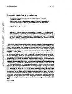
The toy problem of figure 1 consist of 4800 points in D = 2 dimensions whose angular distribution is uniform and whose radial distribution is normal with variance 0.25; θ ∼ U[0, 2π] 17
r ∼ N[R, 0.25] , we generated half the points with R = 3, one third with R = 2 and one sixth with R = 1. 4
2
0
-2
Outer Cluster Central Cluster Inner Cluster Unclassified Points -4
-4
-2
0
2
4
Figure 1: Data distribution: the angular coordinate is uniformly distributed, i.e U[0, 2π], while the radial one is normal N[R, 0.25] distributed around three different radius R. The outer cluster (R = 3.0) consists of 2400 points, the central one (R = 2.0) of 1600 and the inner one (R = 1.0) of 800. The classified data set: points classified at T = 0.05 as belonging to the three largest clusters are marked by circles (outer cluster, 2358 points), squares (central cluster, 1573 points) and triangles (inner cluster, 779 points). The x’s denotes the 90 remaining points which are distributed in 43 clusters, the biggest of size 4.
Since there is a small overlap between the clusters, we consider the Bayes solution as the optimal result; i.e. points whose distance to the origin is bigger than 2.5 are considered a cluster, points whose radial coordinate lies between 1.5 and 2.5 are assigned to a second cluster and the remaining points define the third cluster. These optimal clusters consist of 2393, 1602 and 805 points respectively. 18
By applying our procedure, and choosing the neighbors according to the mutual neighborhood criterion with K = 10 we obtain the susceptibility as a function of the temperature as presented in figure 2(a). The estimated temperature (10) corresponding to the superparamagnetic to paramagnetic transition is 0.075, which is in a good agreement with the one inferred from figure 2(a).
0.050
(a)
χT/N
0.040 0.030 0.020 0.010 0.000
0.00
0.02
0.04
0.06
0.08
0.10
5000
(b) Cluster Size
4000 3000 outer cluster
2000
central cluster
st
1000 0 0.00
1 cluster nd 2 cluster rd 3 cluster th 4 cluster
0.02
inner cluster
0.04
0.06
0.08
0.10
T
Figure 2: (a) The susceptibility density
χT N
of the data set of figure 1 as a function of the
temperature. (b) Size of the four biggest clusters obtained at each temperature.
Figure 1 presents the clusters obtained at T = 0.05. The sizes of the three largest clusters are 2358, 1573 and 779 including 98% of the data; the classification of all these points coincides with that of the optimal Bayes classifier. The remaining 90 points are 19
distributed among 43 clusters of size smaller than 4. As can be noted in figure 1, the small clusters (less than 4 points) are located at the boundaries between the main clusters. One of the most salient features of the SPC method is that the spin–spin correlation function, Gij reflects the existence of two categories of neighboring points: neighboring points that belong to the same cluster and those that do not. This can be observed from figure 3(b), the two-peaked frequency distribution of the correlation function Gij between neighboring points of figure 1. In contrast, the frequency distribution 3(a) of the normalized distances
dij a
between neighboring points of figure 1, contains no hint of the existence of a
natural cutoff distance, that separates neighboring points into two categories. 4000
24000
(a)
(b)
22000 3000
8000 2000
6000
4000 1000
2000
0 0.0
1.0
dij/a
2.0
3.0
1/q
1
Gij
Figure 3: Frequency distribution of (a) distances between neighboring points of fig. 1 (scaled by the average distance a), and (b) spin–spin correlation of neighboring points.
It is instructive to observe the behavior of the size of the clusters as a function of the temperature, presented in figure 2(b). At low temperatures, as expected, all data points form only one cluster. At the ferromagnetic to super-paramagnetic transition temperature, indicated by a peak in the susceptibility, this cluster splits into three. These essentially remain stable in their composition until the super-paramagnetic to paramagnetic transition temperature is reached, expressed in a sudden decrease of the susceptibility χ, where the clusters melt. Turning now to the effect of the parameters on the procedure, we found (Wiseman et. al. 1996) that the number of Potts states q affects the sharpness of the transition but the obtained classification is almost the same. For instance, choosing q = 5 we found that the 20
three largest clusters contained 2349, 1569 and 774 data points, while taking q = 200 we yielded 2354, 1578 and 782. Of all the algorithms listed at the beginning of this section, only the single–link and minimal spanning methods were able to give (at the optimal values of their clustering parameter) a partition that reflects the underlying distribution of the data. The best results are summarized in table 1, together with those of the SPC method. Clearly, the standard parametric methods (such k-means or Ward’s method) would not be able to give a reasonable answer because they assume that different clusters are parameterized by different centers and a spread around them. Method
outer
central
inner
unclassified
cluster
cluster
cluster
points
Bayes
2393
1602
805
–
Super–Paramagnetic (q=200)
2354
1578
782
86
Super–Paramagnetic (q= 20)
2358
1573
779
90
Super–Paramagnetic (q= 5)
2349
1569
774
108
Single–Link
2255
1513
758
274
Minimal Spanning Tree
2262
1487
756
295
Table 1: Clusters obtained with the methods that succeeded in recovering the structure of the data. Points belonging to cluster of sizes less than 50 points are considered as “unclassified points”. The Bayes method is used as benchmark because it is the one that minimizes the expected number of mistakes, provided that the distribution that generated the set of points is known
In figure 4 we present, for the methods that depend only on a single parameter, the sizes of the four biggest clusters that were obtained as a function of the clustering parameter. The best solution obtained with the single–link method (for a narrow range of the parameter) corresponds also to three big clusters of 2255, 1513 and 758 points respectively, while the remaining clusters are of size smaller than 14. For larger threshold distance the second and third clusters are linked. This classification is slightly worse than the one obtained by the super–paramagnetic method. 21
When comparing SPC with single–link one should note that if the “correct” answer is not known, one has to rely on measurements such as the stability of the largest clusters (existence of a plateau) to indicate the quality of the partition. As can be observed from figure 4(a) there is no clear indication that signals which plateau corresponds to the optimal partition among the whole hierarchy yielded by single link. The best result obtained with
(b) directed graph
cluster size
(a) single linkage 5000
5000
4000
4000
3000
3000
2000
2000
1000
1000
0.06
0.08
0.10
0.12
0.14
0.30
cluster size
(c) complete linkage 5000
5000
4000
4000
3000
3000
2000
2000
1000
1000
1.0
3.0
5.0
7.0
6
cluster size
5000
5000
4000
4000
3000
3000
2000
2000
1000
1000
0.80
1.00
1.20
clustering parameter
0.90
1.20
7
8
9
10
(f) shared neighborhood
(e) valey seeking
0.60
0.60
(d) mutual neighborhood
1.40
11
12
13
14
clustering parameter
Figure 4: Size of the three biggest clusters as a function of the clustering parameter obtained with (a) single–link, (b) directed graph, (c) complete–link, (d) mutual neighborhood, (e) valley seeking and (f ) shared neighborhood algorithm. The arrow in (a) indicate the region corresponding to the optimal partition for the single–link method. The other algorithms were unable to recover the data structure.
the minimal spanning tree method is very similar to the one obtained with the single– link, but this solution corresponds to a very small fraction of its parameter space. In comparison, SPC allows clear identification of the relevant super–paramagnetic phase; the entire temperature range of this regime yields excellent clustering results. 22
5.2
Only one cluster
Most existing algorithms impose a partition on the data even when there are no natural classes present in it. The aim of this example is to show how the SPC algorithm signals this situation. Two different 100–dimensional data sets of 1000 samples are used. The first data set is taken from a Gaussian distribution centered at the origin, with covariance matrix equal to the identity. The second data set consists of points generated randomly from a uniform distribution in a hypercube of side 2. The susceptibility curve, which was obtained by using the SPC method with these data sets is shown in figures 5(a) and 5(b). The narrow peak and the absence of a plateau Gaussian Distribution
Uniform Distribution 0.008
0.03
(a)
(b) 0.006
χT/N
0.02 0.004 0.01 0.002
0.00 0.00
0.05
0.10
0.15
0.20
0.25
1000
0.000 0.00
cluster size
(c)
0.10
0.05
0.10
0.15
0.20
0.25
0.15
0.20
0.25
(d)
750
750
500
500
250
250
0 0.00
0.05
1000
0.05
0.10
0.15
0.20
0 0.00
0.25
T
Figure 5: Susceptibility density
T
χT N
as a function of the temperature T for data points
(a) uniformly distributed in a hypercube of side 2 and (b) multi-normally distributed with covariance matrix equal to the identity in a 100-dimensional space. The size of the two biggest clusters obtained at each temperature are presented in (c) and (d) respectively.
indicate that there is only a single phase transition (ferromagnetic to paramagnetic), with no super-paramagnetic phase. This single phase transition is also evident from figures 5(c) and 5(d) where only one cluster of almost 1000 points appears below the transition. This single “macroscopic” cluster “melts” at the transition, to many “microscopic” clusters of 23
1–3 points in each.
Clearly, all existing methods are able to give the correct answer since it is always possible to set the parameters such that this trivial solution is obtained. Again, however, there is no clear indicator for the correct value of the control parameters of the different methods.
5.3
Performance: scaling with data dimension and influence of irrelevant features
The aim of this example is to show the robustness of the SPC method and to give an idea of the influence of the dimension of the data on its performance. To this end we generated N D–dimensional points whose density distribution is a mixture of two isotropic Gaussians, i.e.
P(~x)
√ �−D � � � �� � 2πσ k~x − ~y2 k2 k~x − ~y1 k2 + exp − exp − = 2 2σ 2 2σ 2
(12)
where ~ y1 and ~y2 are the centers of the Gaussians and σ determines its width. Since the two characteristics lengths involved are k~y1 − ~y2 k and σ, the relevant parameter of this example is the normalized distance L =
k~ y1 −~ y2 k . σ
The manner in which these data points were generated satisfies precisely the hypothesis about data distribution that is assumed by the K-means algorithm. Therefore it is clear that this algorithm (with K=2) will achieve the Bayes optimal result; the same will hold for other parametric methods, such as maximal likelihood (once a two-Gaussian distribution for the data is assumed). Even though such algorithms have, for this kind of data, an obvious advantage over SPC, it is interesting to get a feeling about the loss in the quality of the results, caused by using our method, which relies on less assumptions. To this end we considered the case of 4000 points generated in a 200–dimensional space from the distribution (12), setting the parameter L = 13.0 σ. The two biggest clusters we obtained were of sizes 1853 and 1816; the smaller ones contained less than 4 points each. About 8.0 % of the points were left unclassified, but all those points that the method did assign to one of the two large clusters, were classified in agreement with a Bayes classifier. For comparison we applied the single linkage algorithm to the same data; at the best classification point 74% of the points were unclassified. 24
Next we studied the minimal distance, Lc , at which the method is able to recognize that two clusters are present in the data and, to find the dependence of Lc on the dimension D and number of samples N . Note that the lower bound for the minimal discriminant distance for any non-parametric algorithm is 2 (for any dimension D). Below this distance the distribution is no longer bimodal, but rather the maximal density of points is located at the at the midpoint between the Gaussian centers. Sets of N = 1000, 2000, 4000 and 8000 samples and space dimensions D = 2, 10, 100, 100 and 1000 were tested. We set the number of neighbors K = 10 and superimposed the minimal spanning tree to ensure that at T = 0 all points belong to the same cluster. To our surprise we observed that in the range 1000 ≤ N ≤ 8000 the critical distance seems to depend only weakly on the number of samples, N . The second remarkable result is that the critical discriminant distance Lc grows very slowly with the dimensionality of the data points, D. Apparently the minimal discriminant distance Lc increases like the logarithm of the number of dimensions D; Lc ≈ α + β log D
(13)
where α and β do not depend on D. The best fit in the range 2 ≤ D ≤ 1000, yields α = 2.3 ± 0.3 and β = 1.3 ± 0.2. Thus, this example suggests that the dimensionality of the points does not affect the performance of the method significantly. A more careful interpretation is that the method is robust against irrelevant features present in the characterization of the data. Clearly, there is only one relevant feature in this problem, which is given by the projection x′ =
~y1 − ~y2 · ~x . k~y1 − ~y2 k
The Bayes classifier, which has the lowest expected error, is implemented by assigning ~xi to cluster 1 if x′i < 0 and to cluster 2 otherwise. Therefore we can consider the other D − 1 dimensions as irrelevant features because they do not carry any relevant information. Thus, equation (13) is telling us how noise, expressed as the number of irrelevant features present, affects the performance of the method. Adding pure noise variables to the true signal can lead to considerable confusion when classical methods are used (Fowlkes et. al. 1988). 25
5.4
The Iris Data
The first “real” example we present is the time–honored Anderson–Fisher Iris data, which has become a popular benchmark problem for clustering procedures. It consists of measurement of four quantities, performed on each of 150 flowers. The specimens were chosen from three species of Iris. The data constitute 150 points in four-dimensional space. The purpose of this experiment is to present a slightly more complicated scenario than that of fig. 1. From the projection on the plane spanned by the first two principal components, presented on fig. 6, we observe that there is a well separated cluster (corresponding to the Iris Setosa species) while clusters corresponding to the Iris Virginia and Iris Versicolor do overlap.
second principal component
5.0
4.0
3.0
2.0 Iris Setosa Iris Versicolor Iris Virginica
1.0 2.0
4.0
6.0 8.0 first principal component
10.0
Figure 6: Projection of the iris data on the plane spanned by its two principal components.
We determined neighbors in the D = 4 dimensional space according to the mutual K (K=5) nearest neighbors definition; applied the SPC method and obtained the susceptibility curve of Fig. 7(a); it clearly shows two peaks! When heated, the system first breaks into two clusters at T ≈ 0.1. At Tclus = 0.2 we obtain two clusters, of sizes 80 and 40; points of the smaller cluster correspond to the species Iris Setosa. At T ≈ 0.6 another transition occurs, where the larger cluster splits to two. At Tclus = 0.7 we identified clusters of sizes 45, 40 26
and 38, corresponding to the species Iris Versicolor,Virginica and Setosa respectively.
(a) 0.20
χT/N
0.15
0.10
0.05
0.00 0.00
cluster size
(b)
0.02
0.04
0.06
0.08
0.10
150 st
100
50
1 cluster nd 2 cluster rd 3 cluster th 4 cluster th 5 cluster
Versicolor + Virginica
Setosa
Setosa Virginica
0 0.00
0.02
0.04
Versicolor
0.06
0.08
0.10
T
Figure 7: (a) The susceptibility density
χT N
as a function of the temperature and (b) the
size of the four biggest clusters obtained at each temperature for the Iris data.
As opposed to the toy problems, the Iris data breaks into clusters in two stages. This reflects the fact that two of the three species are “closer” to each other than to the third one; the SPC method clearly handles very well such hierarchical organization of the data. 125 samples were classified correctly (as compared with manual classification); 25 were left unclassified. No further breaking of clusters was observed; all three disorder at Tps ≈ 0.8 (since all three are of about the same density). Among all the clustering algorithms used in this work, the minimal spanning tree procedure obtained the most accurate result, followed by our method, while the remaining clustering techniques failed to provide a satisfactory result.
27
Method
biggest
middle
smallest
cluster
cluster
cluster
Minimal Spanning Tree
50
50
50
Super–Paramagnetic
45
40
38
Valley Seeking
67
42
37
Complete–Link
81
39
30
Directed Graph
90
30
30
K-Shared Neighbors
90
30
30
Single–Link
101
30
19
Mutual Neighborhood Value
101
30
19
Table 2: Best partition obtained with each of the clustering methods. Only the minimal spanning tree and the super–paramagnetic method returned clusters where points belonging to different Iris species were not mixed
5.5
LANDSAT data
Clustering techniques have been very popular in remote sensing applications (Faber et. al.
1994, Kelly and White 1993, Kamata and Kawaguchi 1995; Larch 1994, Kamata
et. al.
1991). Multi-spectral scanners on LANDSAT satellites sense the electromagnetic
energy of the light reflected by the earth’s surface in several bands (or wavelengths) of the spectrum. A pixel represents the smallest area on earth’s surface that can be separated from the neighboring areas. The pixel size and the number of bands varies, depending on the scanner; in this case four bands are utilized, whose pixel resolution is of 80 × 80 meters. Two of the wavelengths are in the visible region, corresponding approximately to green (0.52 to 0.60 µm ) and red (0.63 to 0.69µm ) and the other two are in the near–infrared (0.76 to 0.90 µm ) and mid–infrared (1.55 to 1.75 µm ) regions. The wavelength interval associated with each band is tuned to a particular cover category. For example the green band is useful for identifying areas of shallow water, such as shoals and reefs, whereas the red band emphasizes urban areas. The data consist of 6437 samples that are contained in a rectangle of 82 × 100 pixels. Each “data point” is described by 36 features that correspond to a 3 × 3 square of pixels. 28
A classification label (ground truth) of the central pixel is also provided. The data is given in random order and certain samples have been removed, so that one cannot reconstruct the original image. The data was provided by Srinivasan (1994) and is available at the UCI Machine Learning Repository (Murphy and Aha 1994). The goal is to find the “natural classes” present in the data (without using its labels, of course). The quality of our results is determined by the extent to which the clustering reflects the six terrain classes present in the data: red soil, cotton crop, grey soil, damp grey soil, soil with vegetation stubble and very damp grey soil. This exercise is close to a real problem of remote sensing, where the true labels (ground truth) on the pixels is not available, and therefore clustering techniques are needed to group pixels on the basis of the sensed observations.
100
cotton crop 60
red soil 20
-20
grey soil very damp grey soil damp grey soil soil with vegetation subble -20
20
60
100
Figure 8: Best two dimensional projection pursuit among the first six solutions for the LANDSAT data
We used the projection pursuit method (Friedman 1987), which is a dimension–reducing 29
transformation, in oder to gain some knowledge about the organization of the data. Among the first six two–dimensional projections that were produced we present in figure 8 that one which reflects best the (known) structure of the data. We observe the that: (a) the clusters differ in their density, (b) there is unequal coupling between clusters, and (c) the density of the points within a cluster is not uniform; it decreases towards the perimeter of the cluster.
(2)
0.010
χT/N
0.008 0.006 0.004
(4)
0.002 0.000
(3)
(1)
0.04
0.06
0.08
0.10
0.12
0.14
0.16
7000 st
cluster size
6000
1 cluster nd 2 cluster rd 3 cluster th 4 cluster
A
5000 A2
4000 3000
1
A2 : grey soil 2
2000 1000 0
A2 : very damp grey soil
A1 : red soil
3
A1
B: cotton crop
0.04
0.06
0.08
0.10
0.12
A2 : damp
1
A1
2 4
A2 : vegetation
0.14
0.16
T
Figure 9: (a) Susceptibility density
χT N
of the Landsat data as a function of the temperature
T. The number in parenthesis indicate the phase transitions. (b) The sizes of the four biggest clusters at each temperature. The jumps indicate that a cluster has been split. Symbols A,B,Ai and Aji corresponds to the hierarchy depicted in fig. 10 .
The susceptibility curve Fig. 9(a) reveals four transitions, that reflect the presence of the following hierarchy of clusters (see fig. 10). At the lowest temperature two clusters A and B appear. Cluster A splits at the second transition into A1 and A2 . At the next transition cluster A1 splits into A11 and A21 . At the last transition cluster A2 splits into four clusters Ai2 , i = 1...4. At this temperature the clusters A2 and B are no longer identifiable; their 30
spins are in a disordered state, since the density of points in A2 and B is significantly smaller than within the Ai1 clusters. Thus the super–paramagnetic method overcomes the difficulty of dealing with clusters of different densities by analyzing the data at several temperatures. This hierarchy indeed reflects the structure of the data. Clusters obtained in the range of
(1)
A
(2)
A1
(3)
1
A2
A1
red soil
2
A1
B cotton crop
(4)
1
2
A2
A2
grey soil
very damp
3
A2
4
A2
damp vegetation g.s.
Figure 10: The Landsat data structure reveals a hierarchical structure. The number in parenthesis corresponds to the phase transitions indicated by a peak in the susceptibility (fig. 9)
temperature 0.08 to 0.12 coincides with the picture obtained by projection pursuit; cluster B corresponds to cotton crop terrain class, A1 to red soil and the remaining four terrain classes are grouped in the cluster A2 . The clusters A11 and A21 are a partition of the red soil4 , while A12 , A22 , A32 and A42 correspond, respectively, to the classes grey soil, very damp grey soil, damp grey soil and soil with vegetation stubble. 97% purity was obtained, meaning that points belonging to different categories were almost never assigned to the same cluster. Only the optimal answer of Fukunaga’s valley seeking, and our SPC method succeeded in recovering the structure of the LANDSAT data. Fukunaga’s method, however, yielded for 4
This partition of the red soil is not reflected in the “true” labels. It would be of interest to reevaluate the
labeling and try to identify the features that differentiate the two categories of red soil that were discovered by our method.
31
different (random) initial conditions grossly different answers, while our answer was stable.
5.6
Isolated Letter Speech Recognition
In the isolated–letter speech recognition task, the “name” of a single letter is pronounced by a speaker. The resulting audio signal is recorded for all letters of the English alphabet for many speakers. The task is to find the structure of the data, which is expected to be a hierarchy reflecting the similarity that exists between different groups of letters, such as {B, D} or {M, N } which differ only in a single articulatory feature. This analysis could be useful, for instance, to determine to what extent the chosen features succeed in differentiating the spoken letters. We used the ISOLET database of 7797 examples created by Ron Cole (Fanty and Cole 1991) which is available at the UCI machine learning repository (Murphy and Aha 1994). The data was recorded from 150 speakers balanced for sex and representing many different accents and English dialects. Each speaker pronounce each of the 26 letters twice (there are 3 examples missing). Cole’s group has developed a set of 617 features describing each example. All attributes are continuous and scaled into the range −1 to 1. The features include spectral coefficients, contour features, sonorant, pre–sonorant, and post–sonorant features. The order of appearance of the features is not known. We applied the SPC method and obtained the susceptibility curve shown in figure 11(a) and the cluster size versus temperature curve presented in fig 11(b). The resulting partitioning obtained at different temperatures can be cast in hierarchical form, as presented in fig. 12(a). We also tried the projection pursuit method; but none of the first six 2-dimensional projections succeeded to reveal any relevant characteristic about the structure of the data. In assessing the extent to which the SPC method succeeded to recover the structure of the data, we built a “true” hierarchy by using the known labels of the examples. To do this, we first calculate the center of each class (letter) by averaging over all the examples belonging to it. Then a matrix 26 × 26 of the distances between these centers is constructed. Finally, we apply the single–link method to construct a hierarchy, using this proximity matrix. The result is presented in figure 12(b). The purity of the clustering was again very high (93%); and 35% of the samples were left as unclassified points. The CPCC validation index (Jain 32
0.010
(a) 0.008
χΤ/Ν
0.006
0.004
0.002
0.000
0.04
0.06
0.08
0.10
0.12
0.14
T
8000
(b)
cluster sizes
6000
4000
2000
st
1 cluster nd 2 cluster rd 3 cluster th 4 cluster 0
0.04
0.06
0.08
0.10
0.12
0.14
T
Figure 11: (a) Susceptibility density as a function of the temperature for the isolated–letter speech–recognition data. (b) Size of the four biggest clusters returned by the algorithm for each temperature. 33
and Dubes 1988) is equal to 0.98 for this graph, which indicates that this hierarchy fits very well the data. Since our method does not have a natural length scale defined at each resolution, we cannot use this index for our tree. Nevertheless, the good quality of our tree, presented in figure 12(a), is indicated by the good agreement between it and the tree of Fig. 12(b). Needless to say, in order to construct the “reference” tree depicted in fig.12(b) , the correct label of each point must be known.
6
Complexity and computational overhead
Non-parametric clustering is performed in two main stages: Stage 1: Determination of the “geometrical structure” of the problem. Basically a number of nearest neighbors of each point has to be found, using any reasonable algorithm, such as identifying the points lying inside a sphere of a given radius, or a given number of closest neighbors (like in the SPC algorithm). Stage 2: Manipulation of the data. Each method is characterized by a specific processing of the data. For almost all methods, including SPC, complexity is determined by the first stage because it deserves more computational effort than the data manipulation itself. Finding the nearest neighbors is an expensive task, the complexity of branch and bound algorithms (Kamgar-Parsi and Kanal 1985) is of order O(N ν log N ) (1 < ν < 2). Since this operation is common for all non–parametric clustering methods, any extra computational overhead our algorithm may have over some other non–parametric method must be due to the difference between the costs of the manipulations performed beyond this stage. The second stage, in the SPC method, consists of equilibrating a system at each temperature. In general, the complexity is of order N (Binder and Heermann 1988, Gould and Tobochnik 1988). Scaling with N: The main reason for choosing an unfrustrated ferromagnetic system, versus to a spin–glass (where negative interactions are allowed), is that ferromagnets reach thermal equilibrium very fast. Very efficient Monte Carlo algorithms (Wang and Swendsen 1990, Wolf 1989, Kandel and Domany 1991) were developed for these systems, in which the number of sweeps needed for thermal equilibration is small at the temperatures of interest. 34
(a)
ABCDEFGHIJKLMNOPQRSTUVWXYZ ABCDEFGHIJKLMNOPQRSTUVXYZ ABCDEFGHJKLMNOPSTVXZ ABCDEGJKLMNOPTVZ ABCDEGJKMNPTVZ ABCDEGJKPTVZ
IRY
W W
QU
HFSX
LO
H
W
FSX IR
MN I
Y
U
Q
R
ABDEGJKPTV CZ
W
BDEGJKPTV A BDEGPTV GPT
P
MN
JK CZ
BDEV
GT E
BD V
JK
A
Q
L O FS
O L
C
U
X X I
H FS
R
Y
ABCDEFGHIJKLMNOPQRSTUVWXYZ
(b)
ABCDEFGHIJKLMNOPRSTVXYZ ABCDEFGHIJKLMNOPRSTVXZ
ABCDEGHJKMNPTVZ
MN
ABDEGHJKPTV ABDEGJKPTV
V
BDE BD
E
B D
Figure 12:
GPT P
M
C
Z
U
L
O
FSX FS
IR X
I
R
F S
N
AJK
BDEGPTV BDEGPT
H
LO
CZ
Y Q
W
FIRSX
ABCDEGHJKLMNOPTVZ ABDEGHJKMNPTV
QU
JK
A J
K
GT G
T
Isolated–letter speech–recognition hierarchy obtained by (a) the Super–
Paramagnetic method and (b) using the labels of the data and assuming each letter is well represented by a center. 35
The number of operations required for each Swendsen–Wang Monte Carlo sweep scales linearly with the number of edges; i.e. it is of order K × N (Hoshen and Kopelman 1976). In all the examples of this article we used a fixed number of sweeps (M = 1000). Therefore, the fact that the SPC method relies on a stochastic algorithm does not prevent it from being efficient. Scaling with D: The equilibration stage does not depend on the dimension of the data, D. In fact it is not necessary to know the dimensionality of the data as long as the distances between neighboring points are known. Since the complexity of the equilibration stage is of order N and does not scale with D, the complexity of the method is determined by the search for the nearest neighbors. Therefore, we conclude that the complexity of our method does not exceed that of the most efficient deterministic non–parametric algorithms. For the sake of concreteness, we present the running times, corresponding to the second stage, on an HP–9000 (series K200) machine for two problems: the LANDSAT (sec. 5.5) and ISOLET data (sec. 5.6). The corresponding running times were 1.97 and 2.53 minutes per temperature respectively (0.12 and 0.15 sec per sweep per temperature). Note that there is a good agreement with the discussion presented above; the ratio of the CPU times is close to the ratio of the corresponding total number of edges (18,388 in the LANDSAT and 22,471 in the ISOLET data set), and there is no dependence on the dimensionality . Typical runs involve about 20 temperatures which leads to 40 and 50 minutes of CPU. This number of temperatures can be significantly reduced by using the Monte Carlo histogram method (Swendsen 1993) where a set of simulations at small number of temperatures suffices to calculate thermodynamic averages for the complete temperature range of interest. Of all the deterministic methods we used, the most efficient one is the minimal spanning tree. Once the tree is built, it requires only 19 and 23 seconds of CPU respectively for each set of clustering parameters. However, the actual running time is determined by how long one spends searching for the optimal parameters in the (3–dimensional) parameter space of the method. The other non–parametric methods presented in this paper were not optimized and therefore comparison of their running times could be misleading. For instance, we used Johnson’s algorithm for implementing the single and complete linkage which requires O(N 3 ) operations for recovering all the hierarchy, but faster versions, based on Minimal 36
Spanning trees require less operations. Running Friedman’s projection pursuit algorithm5 , whose results are presented in fig. 8, required 55 CPU minutes for LANDSAT. For the case of the ISOLET data (where D = 617) the difference was dramatic; projection pursuit required more than a week of CPU time, while SPC required about one hour. The reason is that our algorithm does not scale with the dimension of the data D, whereas the complexity of projection pursuit increases very fast with D.
7
Discussion
This work proposes a new approach to non-parametric clustering, based on a physical, magnetic analogy. The mapping onto the magnetic problem is very simple; a Potts spin is assigned to each data point, and short-range ferromagnetic interactions between spins are introduced. The strength of these interactions decreases with distance. The thermodynamic system defined in this way presents different self organizing regimes and the parameter which determines the behavior of the system is the temperature. As the temperature is varied the system undergoes many phase transitions. The idea is that each phase reflects a particular data structure related to a particular length scale of the problem. Basically, the clustering obtained at one temperature that belongs to a specific phase should not differ substantially from the partition obtained at another temperature in the same phase. On the other hand the clustering obtained at two temperatures corresponding to different phases must be significantly different, reflecting different organization of the data. These ordering properties are reflected in the susceptibility χ and the spin–spin correlation function Gij . The susceptibility turns out to be very useful for signaling the transition between different phases of the system. The correlation function Gij is used as a similarity index, whose value is not determined only by the distance between sites vi and vj , but also by the density of points near and between these sites. Separation of the spin–spin correlations Gij into strong and weak, as evident in fig. 3(a), reflects the existence of two categories of collective behavior. In contrast, as shown in figure 3(b), the frequency distribution of distances dij between neighboring points of Fig. 1 does not even hint that a natural cut-off distance, which separates neighboring points into two categories, exists. Since the double peaked 5
We thank Jerome Friedman for allowing public use his program.
37
shape of the correlations’ distribution persists at all relevant temperatures, the separation into strong and weak correlations is a robust property of the proposed Potts model. This procedure is stochastic, since we use a Monte Carlo procedure to “measure” the different properties of the system, but it is completely insensitive to initial conditions. Moreover, the cluster distribution as a function of the temperature is known. Basically, there is a competition between the positive interaction which encourages the spins to be aligned (the energy, which appears in the exponential of the Boltzmann weight, is minimal when all points belong to a single cluster) and the thermal disorder (that assigns a “bonus” that grows exponentially with the number of uncorrelated spins and, hence, with the number of clusters). We have shown that this method is robust in the presence of noise, and that it is able to recover hierarchical structure of the data without enforcing the presence of clusters. We have also confirmed that the super–paramagnetic method is successful in real life problems, where existing methods failed to overcome the difficulties posed by the existence of different density distributions and many characteristic lengths in the data. Finally we wish to re-emphasize the aspect we view as the main advantage of our method: it’s generic applicability. It is likely and natural to expect that for just about any underlying distribution of data one will be able to find a particular method, tailor-made to handle the particular distribution, whose performance will be better than that of SPC. If however, there is no advance knowledge of this distribution, one cannot know which of the existing methods fits best and should be trusted. SPC, on the other hand, will find any ”lumpiness” (if it exists) of the underlying data, without any fine-tuning of its parameters.
Acknowledgments We thank I. Kanter for many useful discussions. This research has been supported by the Germany-Israel Science Foundation (GIF).
Appendix: Clusters and the Potts model The Potts model can be mapped onto a random–cluster problem (Fortuin and Kasteleyn, 1972, Coniglio and Klein 1980, Edwards and Sokal 1988). In this formulation clusters 38
are defined as connected graph components governed by a specific probability distribution. We present here this alternative formulation in order to give another motivation for the super–paramagnetic method as well as to facilitate its comparison to graph based clustering techniques. Consider the following graph based model whose basic entities are bond variables nij = 0, 1 residing on the edges < i, j > connecting neighboring sites vi and vj . When nij = 1 the bond between sites vi and vj is “occupied”, and when nij = 0 the bond is “vacant”. Given a configuration N = {nij }, random–clusters are defined as the vertices of the connected components of the occupied bonds (where a vertex connected to “vacant” bonds only is considered a cluster containing a single point). The random cluster model is defined by the probability distribution W(N ) =
q C (N ) Y nij pij (1 − pij )(1−nij ) , Z
(14)
where C (N ) is the number of clusters of the given bond configuration, the partition sum Z is a normalization constant, and the parameters pij fulfill 1 ≥ pij ≥ 0. The case q = 1 is the percolation model where the joint probability (14) factorizes into a product of independent factors for each nij . Thus the state of each bond is independent of the state of any other bond. This implies for example that the most probable state is found simply by setting nij = 1 if pij > 0.5 and nij = 0 otherwise. By choosing q > 1 the weight of any bond configuration N is no longer the product of local independent factors. Instead the weight of a configuration is also influenced by the spatial distribution of the occupied bonds, since configurations with more random–clusters are given a higher weight. For instance it may happen that a bond nij is likely to be vacant while a bond nkl is likely to be occupied even though pij = pkl . This can occur if the vacancy of nij enhances the number of random–clusters, while sites vk and vl are connected through other (than nkl ) occupied bonds. Surprisingly there is a deep connection between the random–cluster model and the seemingly unrelated Potts model. The basis for this connection (Edwards and Sokal 1988) is a joint probability distribution of Potts spins and bond variables:
P(S,N ) =
� 1 Y � (1 − pij ) (1 − nij ) + pij nij δsi ,sj . Z
39
(15)
The marginal probability W(N ) is obtained by summing P(S,N ) over all Potts spin configurations. On the other hand by setting � � Jij pij = 1 − exp − , T and summing P
(S,N )
(16)
over all bond configurations the marginal probability (3) is obtained.
The mapping between the Potts spin model and the random–cluster model implies that the super–paramagnetic clustering method can be formulated in terms of the random–cluster model. One way to see this is to realize that the SW–clusters are actually the random– clusters. That is the prescription given in Sec. 3 for generating the SW–clusters is defined through the conditional probability P(N |S) = P(S,N )/P(S). Therefore by sampling the spin configurations obtained in the Monte Carlo sequence (according to probability P(S)), the bond configurations obtained are generated with probability W(N ). In addition, remember that the Potts spin–spin correlation function Gij is measured by using equation (11) and relying on the statistics of the SW–clusters. Since the clusters are obtained through the spin–spin correlations they can be determined directly from the random–cluster model. One of the most salient features of the super–paramagnetic method is its probabilistic approach as opposed to the deterministic one taken in other methods. Such deterministic schemes can indeed be recovered in the zero temperature limit of this formulation (equations (14) and (16) ); at T = 0 only the bond configuration N0 corresponding to the ground state, appears with non-vanishing probability. Some of the existing clustering methods can be formulated as deterministic–percolation models (T = 0, q = 1). For instance, the percolation method proposed by Dekel and West (1985) is obtained by choosing the coupling between spins Jij = θ(R − dij ); that is, the interaction between spins si and sj is equal to one if its separation is smaller than the clustering parameter R and zero otherwise. Moreover, the single–link hierarchy (see for example Jain and Dubes, 1988) is obtained by varying the clustering parameter R. Clearly, in these processes the reward on the number of clusters is ruled out and therefore only pairwise information is used in those procedures. Jardine and Sibson (1971) attempted to list the essential characteristics of useful clustering methods and concluded that the single–link method was the only one that satisfied all the mathematical criteria. However, in practice it performs poorly because single–link clusters easily chain together and are often “straggly”. Only a single connecting edge is 40
needed to merge two large clusters. To some extent the super–paramagnetic method overcomes this problem by introducing a bonus on the number of clusters which is reflected by the fact that the system prefers to break apart clusters that are connected by a small number of bonds. Fukunaga’s (1990) valley–seeking method is recovered in the case q > 1 with interaction between spins Jij = θ(R − dij ). In this case, the Hamiltonian (1) is just the class separability measure of this algorithm where a Metropolis relaxation at T = 0 is used to minimize it. The relaxation process terminates at some local minimum of the energy function, and points with the same spin value are assigned to a cluster. This procedure depends strongly on the initial conditions and is likely to stop at a metastable state that does not correspond to the correct answer.
References Ahuja, N. (1982). “Dot pattern processing using Voronoi neighborhood”, IEEE Transactions on Pattern Analysis and Machine Intelligence PAMI 4, 336–343. Ball, G., and Hall, D. 1967. “A clustering technique for summarizing multivariate data”, Behavioral Science 12, 153–155. Baxter, R. J. 1973. “Potts model at the critical temperature”, Journal of Physics C 6, L445–448. Baraldi, A., and Parmiggiani, F. 1995. “A neural network for unsupervised categorization of multivalued input patterns: an application to satellite image clustering”, IEEE Transactions on Geoscience and Remote Sensing 33(2), 305–316. Binder, K., and Heermann, D.W. 1988. Monte Carlo Simulations in statistical physics, an introduction. Springer–Verlag, Berlin Billoire, A., Lacaze, R., Morel, A., Gupta, S.,˙ Irback, A., and Petersson, B. 1991. “Dynamics near a first–order phase transition with the Metropolis and Swendsen–Wang algorithms.” Nuclear Physics B 358, 231 – 248. 41
Blatt, M., Wiseman, S., and Domany, E. 1996a. “Super–paramagnetic clustering of data”, Physical Review Letters 76, 3251–3255. Blatt, M., Wiseman, S., and Domany, E. 1996b. “Clustering data through an analogy to the Potts model” to appear in Advances in Neural Information Processing Systems 8, Touretzky, Mozer, Hasselmo, eds., MIT Press. Blatt, M., Wiseman, S., and Domany, E. 1996c. “Method and apparatus for clustering data”, USA patent application (pending). Buhmann, J.M., and K¨ uhnel, H. 1993. “Vector quantization with complexity costs”, IEEE Transactions Information Theory 39, 1133 (1993). Chen, S., Ferrenberg, A.M., and Landau D.P. 1992. “Randomness–induced second–order transitions in the two–dimensional eight–state Potts model: a Monte Carlo study”, Physical Review Letters, 69 (8), 1213–1215. Coniglio, A., and Klein, W. 1981.
“Thermal phase transitions at the percolation–
threshold”, Physics Letters A 84, 83–84. Cranias, L., Papageorgiou, H.’, and Piperidis, S. 1994. “Clustering: a technique for search space reduction in example–based machine translation”, proceedings of the 1994 IEEE International Conference on Systems, Man, and Cybernetics. Humans, Information and Technology, 1, 1–6. IEEE, New York. Dekel, A., and West, M.J. 1985. “On percolation as a cosmological test”, The Astrophysical Journal 288, 411–417. Duda, R.O., and Hart, P.E. 1973. Pattern Classification and Scene Analysis. Wiley– Interscience, New York. Edwards, R.G., and Sokal, A.D. 1988.
“Generalization of the Fortuin–Kasteleyn–
Swendsen–Wang representation and Monte Carlo algorithm”, Physical review D 38, 2009–2012. Faber, V., Hochberg, J.G., Kelly, P.M., Thomas, T.R., and White, J.M. 1994. “Concept extraction, a data–mining technique”. Los Alamos Science, 22, 122–149. 42
Fanty, M., and Cole, R. 1991. “Spoken letter recognition”, Advances in Neural Information Processing Systems 3, 220–226. Lippmann, Moody and Touretzky, eds., Morgan– Kaufmann, San Mateo. Foote, J.T., and Silverman, H.F. 1994. “A model distance measure for talker clustering and identification”, proceedings of the 994 IEEE International Conference on Acoustics, Speech and Signal Processing 1, 317–320. IEEE, New York. Fowlkes, E.B., Gnanadesikan, R., and Kettering, J.R. 1988. “Variable selection in clustering”, Journal of classification, 5 205–228. Friedman, J.H. 1987. “Exploratory projection pursuit”, Journal of the American statistical association 82, 249–266. Fu, Y., and Anderson, P.W. 1986. “Applications of statistical mechanics to NP–complete problems in combinatorial optimization”. Journal of Physics A: Math. Gen. 19 1605–1620. Fukunaga, K. 1990. Introduction to statistical Pattern Recognition. Academic Press, San Diego. Fortuin, C.M., and Kasteleyn, P.W. 1972.
“On the random–cluster model”, Physica
(Utrecht), 57, 536–564. Gdalyahu, Y., Weinshall, D., unpublished. Gould, H., and Tobochnik, J. 1989. An introduction to computer simulation methods, part II. Addison–Wesley, New York. Gould, H., and Tobochnik, J. 1989. “overcoming critical slowing down”, Computers in physics 82–86. Hennecke, M, and Heyken, U. 1993. “Critical–dynamics of cluster algorithms in the diluite Ising–model”, Journal of Statistical Physics 72, 829–844. Hertz, J., Krogh, A., and Palmer, R. 1991. Introduction to the theory of neural computation Addison–Wesley, Redwood City. 43
Hoshen, J. and Kopelman, R. 1976. “Percolation and cluster distribution. I. Cluster multiple labeling technique and critical concentration algorithm” Physical Review B 14, 3438–3445. Iokibe, T. 1994. “A method for automatic rule and membership function generation by discretionary fuzzy performance function and its application to a practical system”, Proceedings of the First International Joint Conference of the North American Fuzzy Information Processing Society Biannual Conference. The Industrial Fuzzy Control and Intelligent Systems Conference, and the NASA Joint Technology Workshop on Neural Networks and Fuzzy Logic., 363–364. Hall, Hao Ying, Langari and Yen, eds., IEEE, New York. Jain, A.K., and Dubes, R.C. 1988. Algorithms for Clustering Data. Prentice–Hall, Englewood Cliffs. Kamata, S., Eason, R.O., Kawaguchi, E. 1991. “ Classification of Landsat image data and its evaluation using a neural network approach”, Transactions of the Society of Instrument and Control Engineers 27(11), 1302–1306. Kamgar-Parsi, B., Kanal, L.N. 1985. “An improved branch and bound algorithm for computing k–nearest neighbors, Pattern recognition letters 3, 7–12. Kamata, S., Kawaguchi, E., Niimi, M. 1995. “An interactive analysis method for multidimensional images using a Hilbert curve”, Systems and Computers in Japan, 83–92. Kandel, D., and Domany, E. 1991. “General cluster Monte Carlo Dynamics”, Physical Review B 43, 8539–8548. Karayiannis, N.B. 1994. “Maximum entropy clustering algorithms and their application in image compression”, proceedings of the 1994 IEEE International Conference on Systems, Man, and Cybernetics. Humans, Information and Technology 1, 337–342. IEEE, New York. Kelly, P.M., and White, J.M., 1993. “preprocessing remotely–sensed data for efficient analysis and classification”. SPIE Applications of artificial intelligence 1993: knowledge based systems in aerospace and industry. 24–30. 44
Kirkpatrick, S., Gelatt Jr., C.D., and Vecchi, M.P. 1983. “Optimization by simulated annealing”, Science 220, 671–680. Kosaka, T., and Sagayama, S. 1994. “Tree–structured speaker clustering for fast speaker adaptation”, proceedings of the 1994 IEEE International Conference on Acoustics, Speech and Signal Processing 1, 245–248. IEEE, New York. Larch, D. 1994. “ Genetic algorithms for terrain categorization of Landsat”, Proceedings of the SPIE – The International Society for Optical Engineering 2231, 2–6. MacQueen, J. 1967. “Some methods for classification and analysis of multivariate observations”, proceedings of the Fifth Berkeley Symp. Math. Stat. Prob. I, 281–297. M´ezard, M., and Parisi, G. 1986. “A replica analysis of the traveling salesman problem”, Journal de Physique 47, 1285–1286. Miller, D., and Rose, K. 1996. “Hierarchical, unsupervised learning with growing via phase transitions”, Neural Computation, 8, 425–450. Moody, J., and Darken, C.J. 1989. “Fast learning in neural networks of locally–tuned processing units”, Neural Computation 1, 281–294. Murphy, P.M., and Aha.
D.W. (1994). UCI repository of machine learning databases,
http://www.ics.edu/˜ mlearn/MLRepository.html, Irvive, CA: University of California, Department of Information and Science. Niedermayer, F. 1990. “Improving the improved estimators in O(N) spin models”, Physical Letters B 237, 473–475. Nowlan, J.S., and Hinton, G.E. 1991. “Evaluation of adaptive mixtures of competing experts”, Advances in Neural Information Processing Systems 3, 774–780. Lippmann, Moody and Touretzky, eds., Morgan–Kaufmann, San Mateo. Phillips, W.E., Velthuizen, R.P., Phuphanich, S., Hall, L.O., Clarke, L.P., and Silbiger, M.L. 1995. “Application of fuzzy c–means segmentation technique for tissue differentiation in MR images of a hemorrhagic glioblastoma multiforme”, Magnetic Resonance Imaging 13, 277–290. 45
Rose, K., Gurewitz, E., and Fox, G.C. 1990. “Statistical mechanics and phase transitions in clustering”, Physical Review Letters 65, 945–948. Srinivasan A. 1994. UCI Repository of machine learning databases (University of California, Irvine) maintained by P. Murphy and D. Aha (1994). Suzuki, M., Shibata, M., and Suto, Y. 1995. “ Application to the anatomy of the volume rendering–reconstruction of sequential tissue section for rat’s kidney”, Medical Imaging Technology 13, 195–201. Swendsen, R.H., Wang, S., and Ferrenberg, A.M. 1992. “New Monte Carlo methods for improved efficiency of computer simulations in statistical mechanics” in The Monte Carlo method in condensed matter physics, Topics in applied physics 71, 75–91. Edited by K. Binder, Springer–Verlag, Berlin. Swendsen, R.H. 1993. “Modern methods of analyzing Monte Carlo computer simulations”, Physica A 194, 53–62. Wang, S., and Swendsen, R.H. 1990. “Cluster Monte Carlo algorithms”, Physica A 167, 565–579. Wiseman, S., Blatt, M., and Domany, E. 1996. Preprint. Wolff, U. 1989. “Comparison between cluster Monte Carlo algorithms in the Ising spin model”, Physics Letters B 228, 379–382. Yuille, A.L., and Kosowsky, J.J. 1994. Neural Computation 6, 341–356. Wong, Y-F. 1993. “Clustering data by melting”, Neural Computation 5 89–104. Wu, F.Y., 1982. “The Potts model”, Reviews of modern physics, 54(1)235–268.
46