DATA COMPRESSION USING WAVELETS - Purdue Math

DATA COMPRESSION USING WAVELETS: ERROR, SMOOTHNESS, AND QUANTIZATION* Extended Abstract ¨ RONALD A. DeVORE,1 BJORN JAWERTH,1 and BRADLEY J. LUCIER 2 Abstract. Recently, a theory, developed by DeVore, Jawerth, and Popov, of nonlinear approximation by both orthogonal and nonorthogonal wavelets has been applied to problems in surface and image compression by DeVore, Jawerth, and Lucier. This theory relates precisely the norms in which the error is measured, the rate of decay in that error as the compression decreases, and the smoothness of the data. In addition, one can interpret the error incurred by the quantization of wavelet coefficients in terms of this theory. In this talk we give an overview of the previous results, and expand our argument, made earlier for image compression, that frequency-amplitude response curves that arise quite naturally in problems involving human visual and audio perception should be used to decide the quantization strategy for wavelet coefficients and the norm in which to measure the error in compressed data.

1. Introduction In this talk we present an overview of recent theoretical results about methods of data compression based on wavelet decompositions. This theory, developed by DeVore, Jawerth, and Popov [5], relates precisely a one-parameter family of norms used to measure the error between the original and compressed data, the rate of decrease in this error as more coefficients are included in the approximation, and the smoothness of images in certain smoothness classes called Besov spaces. We recall how this theory has been applied to surface compression [4] and image compression [3]. The paper on image compression emphasizes how coefficient quantization strategies can be interpreted in this theory, and, alternately, how the theory can be used to choose a quantization strategy. In addition, [3] introduces the notion that the Contrast Sensitivity Threshold (CST) curve [7], which gives the relationship between contrast and frequency at the limits of human perception, should be used to choose the norm in which to measure the error in compressed images and to choose the quantization strategy. In this talk we explain further how the functional relationship between intensity (or amplitude) and frequency at the limits of human perception in vision or hearing can guide one to choose norms and coefficient quantization strategies to minimize the human perception of error. Furthermore, we emphasize that this theory gives a practical way to measure the smoothness of functions representing surfaces, images, * This work was partially supported by grants from the National Science Foundation and contracts from the Air Force Office of Scientific Research, the Office of Naval Research, the Defense Advanced Research Projects Agency, and the Army High Performance Computing Research Center. 1 Department of Mathematics, University of South Carolina, Columbia, SC 29208 2 Department of Mathematics, Purdue University, West Lafayette, IN 47907

or sound data, using a notion of error that is capable of measuring the smoothness even of the discontinuous, almost fractal, functions that arise, e.g., as image intensities. Finally, we give an explicit series of steps that can be followed to apply this theory to any situation where the perception of a signal or function depends in a known (and hopefully well-behaved) way on both intensity and frequency. 2. Mathematics 2.1. Wavelet decompositions. A wavelet decomposition of a function f defined on Rd is (typically) an expression of the form X (2.1) f= cj,k φj,k , k≥0, j=(j1 ,...,jd )∈Zd

where the coefficients cj,k depend on f and the functions φj,k (x) := φ(2k (x − j/2k )) are the dyadic dilates (by 2k ) and translates (by j/2k ) of a single function φ called a wavelet. (Orthogonal expansions in Rd usually use 2d − 1 functions φ.) We consider a wavelet transform to consist of (1) the functions φj,k and (2) a particular method of choosing the coefficients cj,k . (If the functions φj,k are redundant, or linearly dependent, then there may be more than one way to calculate the coefficients cj,k .) When wavelet decompositions are used as a basis for compressing digitized image or sound data, or surface data that is sampled from a model, we must associate a function f defined on Rd to discrete data that is defined only at the sample points. While one could associate to each data set a function f that is independent of the wavelet transform being applied, it is more amenable to our analysis to allow the representation to depend on the transform; often a discrete transform is applied to the discrete data to get coefficients cj,k , and we define f by (2.1). We then view the data compression problem as one of approximating f by a second (compressed) function f˜. For a lossless algorithm, the original and compressed functions will be the same and the error between them will be zero. We will generally consider algorithms that introduce differences between the original and compressed data in order to achieve higher compression levels. Given the wavelet decomposition, which we consider to be determined by the functions φj,k and the method of choosing the coefficients cj,k , the algorithm calculates quantized coefficients c˜j,k , and the compressed function takes the form X (2.2) f˜ = c˜j,k φj,k . The method of quantizing coefficients involves applying a strategy, which we consider fixed, that depends on one or more parameters, which are allowed to vary. We store or transmit a coded representation of the coefficients c˜j,k , typically through some type of entropy coding. In the following sections we examine and discuss the mathematical issues treated in the earlier paper [5] together with the applications and extensions to the problems of image and surface compression found in [3], [4].

2.2. Error metrics. Based on the intended application, one must decide how to measure the error between f and f˜, which we assume to be defined on some interval I in Rd . (For example, d = 1 for audio data and d = 2 for image or surface data.) There are many possible choices of such a metric; we will use (somewhat arbitrarily) the Lp (I) norms with 0 < p ≤ ∞ as error metrics. These norms, defined by Z 1/p p ˜ ˜ kf − f kLp (I) := |f (x) − f (x)| dx , I

include as special cases the mean square error Z 1/2 2 kf − f˜kL2 (I) := |f (x) − f˜(x)| dx , I

the mean absolute error kf − f˜kL1 (I) :=

Z |f (x) − f˜(x)| dx, I

and the maximum error kf − f˜kL∞ (I) := max |f (x) − f˜(x)|. x∈I

The parameter p gives added flexibility, in that the relative sizes of the component functions cj,k φj,k with amplitude cj,k and frequency 2k , given by kcj,k φj,k kLp (I) , can be changed by varying the parameter p. In other words, varying p allows us to change the relative importance of amplitude and frequency in measuring the size of basic functions. One error metric will not suffice for all applications. For surface compression it is natural to choose the L∞ (I) metric, because two parts that are to fit together must be machined to a certain fixed tolerance. For image compression, one hopes to choose an error metric that parallels the human visual system, so that image differences judged to be large by the human eye are mathematically large and image differences which, for whatever reason, are insignificant to the eye will have small size in the error metric. There is a similar design issue for audio data. One important property of both the human visual and auditory systems is that the lower threshold of perceiving a signal depends on both the intensity and the spatial or temporal frequency of that signal. We argue in §3.1 that these intensity-frequency curve at the threshold of human perception can profitably be used to choose an error metric for data compression. 2.3. Algorithm efficiency and smoothness of data. After deciding on a space X whose metric k · kX will be used to measure the error between f and f˜, we address the question of how to measure the efficiency of a given algorithm. Recall that an algorithm depends on three things: the choice of representation functions φj,k , the method of calculating the coefficients cj,k (which together we call the transform), and the quantization strategy. A given algorithm generates different compressed functions f˜ depending on the parameters of the quantization strategy.

We will compare algorithms on the basis of the error kf − f˜kX and the number of nonzero quantized coefficients c˜j,k . Suppose that a compression algorithm produces a family {f˜} of approximations corresponding to different parameters in the quantization strategy. We introduce for this algorithm the error function aN (f )X :=

inf

f˜ has ≤N coefficients

kf − f˜kX .

In other words, aN measures the compression error that is achieved if the number of coefficients in the compressed function does not exceed N . We ask the following fundamental question: If the φj,k are fixed, how smooth are functions that can be approximated to O(N −α/d ) with ≤ N coefficients by some algorithm that uses the functions φj,k . For the spaces X = Lp and for many classes of representation functions φj,k , DeVore, Jawerth, and Popov [5] have shown that, roughly speaking, (2.3) σN (f )Lp (I) := inf aN (f )Lp (I) = O(N −α/d ) ⇐⇒ f ∈ Bqα (Lq (I)), all algorithms using φj,k

where q = 1/(α/d + 1/p) and the Besov space Bqα (Lq (I)) consists of functions that have α bounded “derivatives” in Lq (I). More precisely, X 1/q ∞ α/d q 1 [N σN (f )Lp (I) ] < ∞ ⇐⇒ f ∈ Bqα (Lq (I)). N N =1

In particular, this is true for box splines [1] (with piecewise constant approximations as a special case) when 0 < p < ∞ and orthogonal wavelets [9], [2] (of which the Haar transform is a special case) when 1 < p < ∞. (Later, DeVore, Petrushev, and Yu [6] extended the results for box splines to the case p = ∞.) So, if we consider N , the number of coefficients in the representation of f˜, to be a measure of the amount of information one must use to represent the compressed data, one can hope to achieve a particular rate of error decay in Lp (I) if and only if f is in a specific Besov smoothness space Bqα (Lq (I)). In proving this theorem, DeVore et al. provide specific algorithms for each set of functions φj,k that give the optimal rate of convergence. One should note that for a wide class of representation functions φj,k , the optimal selection of coefficients for a given α results in the same smoothness classes. The equivalence (2.3) suggests that membership in Besov spaces Bqα (Lq (I)) is an appropriate way of classifying the smoothness of data, in that we can check the effectiveness of a given compression algorithm by seeing how it performs on functions in Bqα (Lq (I)). However, it is of practical interest to measure smoothness in the spaces Bqα (Lq (I)) only if common surfaces, images, or signals are in these spaces. In [3] and [4] evidence is presented that this is indeed the case for surfaces with various singularities and with images. 2.4. Algorithms for data compression. To say that a function f ∈ Bqα (Lq (I)) has enough smoothness to be approximated to O(N −α/d ) in Lp (I) by

functions of the form f˜, does not, in and of itself, explain how to find an algorithm to calculate a particular set of approximations f˜. We briefly describe here a particular algorithm for orthogonal wavelets and indicate how similar algorithms can be constructed for box splines and other wavelets. We restrict our attention for the moment to one dimension. Given any positive value of r, Daubechies [2] and Mallat [8] have shown how to construct a C r function φ such that φj,k (x) := φ(2k x − j), the dyadic dilates and translates of φ, form a complete orthogonal set in L2 (I). (In Rd , there is a set of 2d − 1 such functions that together satisfy this property.) Thus, any function f ∈ L2 (I) can be written as (2.4)

f=

X X < f, φj,k > X φj,k = cj,k φj,k . < φj,k , φj,k >

k∈Z j∈Z

It is clear from the orthogonality of {φj,k } that when approximating f in L2 (I) by P f˜ = c˜j,k φj,k with at most N nonzero terms, then the best choice consists of the N largest values of kcj,k φj,k kL2 (I) , i.e.,  cj,k , for the N largest values of kcj,k φj,k kL2 (I) , c˜j,k = 0, otherwise. In this way we minimize kf − f˜k2L2 (I) =

XX

k(cj,k − c˜j,k )φj,k k2L2 (I) .

k∈Z j∈Z

This suggests that after fixing a positive , one can choose any numbers c˜j,k that satisfy (2.5)

k(cj,k − c˜j,k )φj,k kL2 (I) ≤ 

and we will obtain, if not the best approximation according to our criterion of minimizing the error with a fixed number of nonzero c˜j,k , then at least a good approximation. In fact, from a practical point of view, this flexibility is an asset, for it allows us to choose values of c˜j,k that have a small number of significant bits. The condition (2.5) can be generalized to approximation in Lp (I) in Rd . Under some technical conditions on the wavelets φ and the on the range of α, the following theorem can be proved; see [5], [3]. Theorem 2.1. Choose a positive integer N and numbers 1 < p < ∞ and 0 < α. Let q satisfy q −1 = p−1 + α/d. Write f as (2.4). Choose quantized coefficients c˜j,k that satisfy (2.6)

k(cj,k − c˜j,k )φj,k kqLp (I) ≤

1 . N

(We assume that kcj,k φj,k kqLp (I) ≤ 1/N implies c˜j,k = 0.) Our compressed function is XX f˜ := c˜j,k φj,k . k

j

Then for each 0 < α and 0 < p < ∞ there exist constants C1 and C2 such that for all f ∈ Bqα (Lq (I)): (1) The number, N , of nonzero coefficients c˜j,k satisfies N ≤ C1 N kf kqB α (Lq (I)) .

(2.7)

q

(2) The error f − f˜ satisfies (2.8)

q/p kf − f˜kLp (I) ≤ C2 N −α/d kf kB α (Lq (I)) q

and (2.9)

α/d kf − f˜kLp (I) ≤ C1 C2 N −α/d kf kBqα (Lq (I)) .

The paper by DeVore, Jawerth, and Popov [5] contains extensions of the above theorem to 0 < p < ∞ in the case of box splines. DeVore, Jawerth, and Lucier [3] examine in some detail integer transforms related to the Haar transform for image compression in Lp (I). DeVore, Petrushev, and Yu [6] give a different way to choose the coefficients c˜j,k for box splines so that (2.7), (2.8), and (2.9) hold in L∞ (I). A simpler algorithm for L∞ (I), but which requires greater than optimal smoothness, is contained in [4]. This short list is meant to emphasize that for any p there is an algorithm that will give near-optimal approximation in Lp (I) using wavelets of some kind; the choice of p, which is investigated in §3, depends solely on the application. 2.5. How to choose quantization levels. To transmit images or other signal data along a communications channel, one sends integer codes that represent the quantized coefficients of the transformed data. Here we discuss how to choose quantization levels based on the criterion introduced in Theorem 2.1; this material was also presented in [3]. Specifically, for some N > 0, and a given representation X f= cj,k φj,k , one chooses quantized coefficients c˜j,k such that k(cj,k − c˜j,k )φj,k kqLp (I) ≤

1 , N

or, equivalently, (2.10)

k(cj,k − c˜j,k )φj,k kLp (I) ≤

1 N 1/q

.

Because kφj,k kLp (I) = 2−dk/p kφkLp (I) in Rd , (2.10) says that one should require (2.11)

N 1/q kφkLp (I) 1 |cj,k − c˜j,k | ≤ . 1+dk/p 2 2

Inequality (2.11) implies that when approximating f in Lp (I), one should choose a quantization separation for cj,k+1 that is 2d/p times the quantization separation

for cj,k . Therefore, we can take for coefficients c˜j,k and integer codes codej,k to represent those coefficients,  1/q  N kφkLp (I) 21+dk/p codej,k := round c = codej,k . and c ˜ j,k j,k 21+dk/p N 1/q kφkLp (I) Thus, in two dimensions, as for images, one should reduce by one the number of bits one sends of c˜j,k for each level k to approximate f in L2 (I). To approximate in L1 (I), coefficients c˜j,k+1 should have two fewer significant bits than c˜j,k . In one dimension, as for audio data, one should keep one fewer bit per increased level for approximation in L1 (I), and keep one-half fewer bit per level for approximation in L2 (I) (or at least one should increase the quantization interval by approximately √ 2 for each level). In practice, we suggest setting c˜j,k = cj,k for k less than some fixed level K, and then reducing the number of bits in c˜j,k for higher k according to the formula (2.11). 3. Applications to Data Compression Sometimes an error criterion is externally and unambiguously applied; for example, we would like parts designed by a CAD system to fit together well, and so a maximum tolerance in the design may be specified. For this application one would use an L∞ (I) error criterion. Several applications are given in [4] of wavelet-based compression of surfaces while controlling the maximum error. For other applications, it is the human perception of the compressed data that is most important. DeVore, Jawerth, and Lucier [3] have suggested how to use certain information about the sensitivity of people to visual stimuli at various frequencies and intensities to choose an error metric for image compression that would approximately model this response. Here we expand on this approach and suggest how it can be applied to other situations, such as compressing audio data. 3.1. How human responses to stimuli can lead to the choice of error metric. In §2.4 we gave a general framework for approximating functions f by P ˜ finite linear combinations f = c˜j,k φj,k . This approximation process is nonlinear because the choice of which φj,k to use depends on the function f that will be approximated. The only free parameter in the theory is the parameter p, which determines the error metric. In [3] it is claimed that for image processing one should use the value p = 1. That claim, which is made assuming that the middle frequency information of an image will be kept, is based on the precise way that the threshold of human perception of an oscillating pattern depends on intensity and frequency. Thus, we implicitly assume that the purpose of the images is to “look the best” to a human observer. Here we expand upon that specific claim and show how to choose an error metric in any situation where perception depends in a well-behaved way on both intensity and frequency of sensation. Let us stick with images for a while; at the end we will speculate somewhat on compressing audio signals. P The problem of approximating an image f = cj,k φj,k by wavelets can be

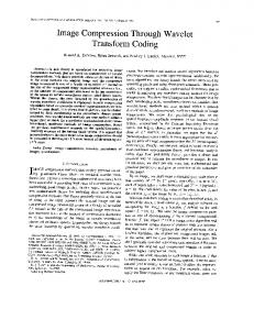
thought of as choosing from among the set of “features” {cj,k φj,k } a finite number {˜ cj,k φj,k }, which, in the case of image compression, should most accurately reflect the visual perception of the image. One quantization strategy that satisfies our theory is simply to order the set {kcj,k φj,k kLp (I) } and choose the N features with the largest norm, so that if kcj,k φj,k kLp (I) ≥ kcl,m φl,m kLp (I) then the “feature” cj,k φj,k will be chosen before cl,m φl,m . One would prefer to choose features that the human eye will find most striking, in some sense, and to leave behind those features that the human visual system does not perceive. Thus, one would like to choose cj,k φj,k before cl,m φl,m if and only if kcj,k φj,k keye ≥ kcl,m φl,m keye , if such a norm could be found. Each feature cj,k φj,k has an intensity of about cj,k and a characteristic frequency of about 2k , as can be seen by examining the Fourier transform of φj,k . It is how people perceive a feature with a certain frequency and contrast that is of primary interest. It is well known that a high frequency pattern superimposed on a grey background will not be discernible from grey, even at high intensity. The threshold of perception of an oscillating pattern of a particular frequency and intensity is known as the Contrast Sensitivity Threshold (CST) curve; see, e.g., [7]. The frequencies to which the human visual system is most sensitive are taken to be the middle frequencies, and people are less able to discern either high frequency or low frequency oscillations from grey. Let us assume that we will keep in our image all mid- and low-frequency information, so our compression problem will be to decide which high-frequency “features” to include in the compressed image. Let us pick a “feature” cφj,k with (high) frequency 2k that is just barely discernible from a grey background. In fact cφl,k+1 will not be discerned from grey; because of the higher frequency, the value of c must be increased to some other value, c¯, to be at the threshold of perception. Thus, in our previous imprecise language, we have kcφj,k keye = k¯ cφl,k+1 keye . The question is, what is the relationship between c and c¯, and is there a value of p such that the same relationship holds for the Lp (I) norm? In fact, for high frequencies, c¯/c = 4, and the only value of p that has the same relationship is p = 1. If c¯/c had been 2, then one could have said that the L2 (I) norm would be better for generating compressed images. But that is not the case. In Figure 1 we present two pictures that have identical levels of compression, the same underlying functions φj,k , the same methods of calculating the coefficients cj,k , and that differ only in whether the L2 or the L1 criterion was used to choose the compressed coefficients c˜j,k . We feel that this L1 picture, among many others, looks better than the L2 picture at the same level of compression. There is a similar threshold curve for audio signals, although it is complicated by the direction the signal is coming from. For high frequencies there is a similar

Figure 1. The left image is compressed using the L2 (I) quantization strategy; it has 4545 nonzero coefficients c˜j,k and 3587 bytes in the compressed file, or 0.109 bits per pixel. The right image uses L1 (I) quantization; it has 4514 nonzero coefficients and the same number of bits per pixel. Even though the images have the same compression rate, each strategy chooses different “features” to keep.

relationship for sounds as for images: if you have a barely perceptible signal with intensity c and frequency 2k , then one must increase the intensity to another value c¯ to hear a signal of frequency 2k+1 . The ratio c¯/c will now determine the norm in which to measure the error in our approximation. Because these signals are onedimensional (d = 1), if c¯/c is 2, then we should approximate in L1 (I); if it is about √ 2 then we should approximate in L2 (I). 3.2. The smoothness of data, and the choice of wavelets. After one has decided on a norm k · kLp (I) for measuring the error in compressed data, one should examine “typical” images or sounds to see which of the smoothness classes Bqα (Lq (I)), 1/q = α/d + 1/p contain these “typical” signals. Note that q depends not only on α and p, but also on the dimension d of the signal, so that different conclusions are possible for one- and two-dimensional signals. The smoothness of the the data one would like to compress is important, because, typically, one must have the rth derivatives of φ bounded for r = bαc if Theorem 2.1 is to hold. Thus, the smoothness of the data determines the smoothness needed in the wavelet. We report in Table 1 the estimated Besov space smoothness of various images compressed using a modified Haar wavelet transform and the L1 (I) coefficient quantization strategy. (See [3] for details.) The images are the green components of color images of “lenna” (in Figure 1), an F-16 flying over mountains, a bridge over a stream in a forest, and an aerial view of an airport and surrounding terrain. If we observe that the error kf − f˜kL1 (I) ≈ CN −β , then we estimate α = 2β and kf kBqα (Lq (I)) = C. (The correlation coefficient indicates the goodness of fit on a loglog scale.) The first two images have a Besov space smoothness of α ≈ 0.6; α ≈ 0.35

for the other images. Because in all cases α < 1, these figures suggest that piecewise constant wavelet approximations achieves the highest rate of approximation for image compression in the L1 (I) metric. That the the latter two images have significantly less smoothness than the first two images expresses mathematically what may be concluded on a purely subjective basis simply by looking at them. Table 1. Estimated Smoothness of Images.

Estimated α Estimated kf kBqα (Lq (I)) Correlation Coefficient

Lenna

F-16

Bridge

Airport

0.599 0.677 −0.999

0.597 0.676 −0.993

0.370 0.571 −0.994

0.306 0.516 −0.992

REFERENCES [1] C. de Boor and R. A. DeVore, Approximation by smooth multivariate splines, Trans. Amer. Math. Soc., 276 (1983), pp. 775-788. [2] I. Daubechies, Orthonormal basis of compactly supported wavelets, Comm. on Pure and Appl. Math., 41 (1988), pp. 909-996. [3] R. A. DeVore, B. Jawerth, and B. J. Lucier, Image compression through wavelet transform coding, preprint. [4] , Surface compression, preprint. [5] R. A. DeVore, B. Jawerth, and V. A. Popov, Compression of wavelet decompositions, preprint. [6] R. A. DeVore, P. Petrushev, and X. M. Yu, Nonlinear wavelet approximations in the space C(Rn ), in Proceedings of the US/USSR Conference on Approximation, Tampa, Springer-Verlag, New York, 1990, to appear. [7] R. F. Hess and E. R. Howell, The threshold contrast sensitivity function in strabismic amblyopia: Evidence for a two type classification, Vision Research, 17 (1977), pp. 1049– 1055. [8] S. Mallat, Multiresolution approximation and wavelet orthonormal bases of L2 (R), Trans. Amer. Math. Soc., 315 (1989), pp. 69–87. [9] Y. Meyer, Wavelets and operators, in Analysis at Urbana I, Proceedings of the Special Year in Modern Analysis at the University of Illinois, 1986–1987, E. R. Berkson, N. T. Peck, and J. Uhl, ed., London Mathematical Society Lecture Notes Series, 137, Cambridge University Press, New York, 1989, pp. 256–365.