Journal of VLSI Signal Processing 18, 287–296 (1998) c 1998 Kluwer Academic Publishers. Manufactured in The Netherlands. °
Image Compression Using KLT, Wavelets and an Adaptive Mixture of Principal Components Model NANDA KAMBHATLA IBM T.J. Watson Research Center, 30 Saw Mill River Road, Hawthorne, NY 10532 SIMON HAYKIN Communications Research Laboratory, McMaster University, 1280 Main St. W., Hamilton, ON L8S 4K1, Canada ROBERT D. DONY School of Engineering, University of Guelph, Guelph, ON N1G 2W1, Canada Received November 15, 1996; Revised June 23, 1997
Abstract. In this paper, we present preliminary results comparing the nature of the errors introduced by the mixture of principal components (MPC) model with a wavelet transform and the Karhunen Lo`eve transform (KLT) for the lossy compression of brain magnetic resonance (MR) images. MPC, wavelets and KLT were applied to image blocks in a block transform coding scheme. The MPC model partitions the space of image blocks into a set of disjoint classes and computes a separate KLT for each class. In our experiments, though both the wavelet transform and KLT obtained a higher peak signal to noise ratio (PSNR) than MPC, according to radiologists, MPC preserved the texture and boundaries of gray and white matter better than the wavelet transform or KLT.
1.
Introduction
In this paper, we compare the nature of the error introduced by the mixture of principal components (MPC) algorithm [1] with wavelets and a JPEG-like algorithm, for lossy compression of magnetic resonance (MR) images of the brain. We present results of this comparison, and briefly discuss extensions of MPC and directions for future research. Transform based algorithms for lossy compression transform an image to concentrate signal energy into a few coefficients, quantize the coefficients, and then entropy code them after assigning special symbols for runs of zeros (run length encoding). Using fixed (signal independent) transforms can be computationally very efficient. However, for the compression of a specific domain of images (e.g., brain MR images), signal dependent transforms which learn the statistical commonality between images within the domain, can generate better results.
The Karhunen-Lo`eve transform (KLT) is a signal dependent linear transform which computes the principal components of input data (pixel intensities within an image block) along eigen-directions of the input autocorrelation matrix. The JPEG standard [2] uses a linear transform, the discrete cosine transform [3], a signal independent approximation to the Karhunen-Lo`eve transform (KLT) whose performance is asymptotically equivalent. Another commonly used linear transform is the wavelet transform. The FBI recently adopted a wavelets based technique, called “wavelet/scalar quantization” (WSQ) [4] as the standard for compression of digitized fingerprints. The KLT is the optimal linear transform for energy compaction into a few coefficients. However, the KLT only decorrelates the image pixels within a block. Further, the usefulness of linear techniques on images can be limited due to the presence of nonlinear features in images. For example, the human visual system, which can outperform any artificial vision system in all but
288
Kambhatla, Haykin and Dony
the most trivial tasks, gains much of its power through the many nonlinear stages of processing and representation [5]. The mixture of principal components (MPC) model [1] learns a non-linear model as a mixture of linear transforms. MPC partitions the space of image blocks into a set of disjoint classes and computes a separate KLT for each class, retaining only a few coefficients. We applied KLT, WSQ and MPC for the compression of brain MR images at various degrees of compression and measured the squared error distortion. Futher, the nature of the distortion was compared by examining the test image compressed to the same degree by the various techniques. As a final comparison, these reconstructed images were shown to radiologists at the McMaster University Medical Centre. Though the WSQ and KLT images obtained a lower mean squared error than MPC, the radiologists observed that the MPC reconstructed images better preserved the features useful for diagnosis. This paper is organized as follows. Section 2 details the wavelet compression method (WSQ) used in this investigation and Section 3 describes the MPC algorithm. In Section 4, we describe experimental results comparing KLT, WSQ, and MPC for compression of brain MR images. We discuss directions for future research in Section 5 and present our conclusions in Section 6.
2.
Image Compression Using Wavelets: The Wavelet/Scalar Quantization (WSQ) Algorithm
Wavelet analysis is the computation of components of data along dilated and shifted versions of a pair of low pass and high pass filters (called the scaling function and mother wavelet). Figure 1 shows a perfect reconstruction two channel filter bank. Here, H0 and H1 are, respectively, the low pass and high pass filters of the analysis filter bank and F0 and F1 are the corresponding biorthogonal filters for the synthesis filter bank. Let
Figure 1. A two channel perfect reconstruction filter bank. The analysis filter decomposes an n-dimensional vector x into an n/2dimensional vector a0 and an n/2-dimensional vector a1 . After upsampling and applying the synthesis filter bank, the vector x is recovered exactly.
x be an n-dimensional vector (for now, assume that n is even). The analysis filter bank followed by downsampling gives us an n/2-dimensional vector a0 and an n/2-dimensional vector a1 . The filter banks are chosen such that after up-sampling (inserting zeros) and applying the synthesis filter bank, we can reconstruct x exactly. Thus, we obtain a size preserving decomposition into two frequency subbands (a0 and a1 ), such that the total size is still n. By recursively feeding the output of the low pass filter (a0 ) back through the analysis filter bank, we can obtain a dyadic frequency decomposition. Thus, the wavelet transform can be considered to be a form of subband coding using a cascaded set of two channel filter banks. A number of wavelet approaches exist [6]. While their basis functions differ, they use the same basic model of multiresolution decomposition. For this evaluation, a standard technique recently adopted by the FBI was used. This method is referred as wavelet/scalar quantization (WSQ), and is the standard for digitized fingerprint compression [4]. A WSQ encoder decomposes an image into 64 frequency subbands by recursively applying a low pass filter and a high pass filter (a two channel filter bank) to symmetric extensions of image rows and columns. Using symmetric extensions ensures that the original image size can be arbitrary and does not add variance to high frequency subbands as is the case when using circular convolution. The analysis and synthesis filter banks are 7- and 9-tap symmetric biorthogonal wavelet bases constructed by Cohen et al. [7]. The analysis filter bank is applied to image rows, and then to columns, resulting in four frequency subbands. The filter bank is applied recursively to downsampled subband coefficients to yield the 64 subband decomposition shown in Fig. 2. Using
Figure 2. The 64 frequency subbands decomposition obtained by recursively applying a two channel perfect reconstruction filter bank, as specified in the WSQ standard.
Image Compression
symmetric linear phase filters ensures that the transform is nonexpansive. Thus, we end up with a transform matrix of the same size as the input image. After transforming an image, WSQ scalar quantizes the transform coefficients uniformly. For simplicity, we used the same quantization step size for all coefficients in all subbands. We used special symbols for runs of zeros of size 1–100, quantized coefficients between −73 and 74, and escape sequences for coefficients outside this range, and then Huffman coded these symbols. The exact steps used by WSQ are described in [8]. The FBI obtained archival quality images using between 15 : 1 and 20:1 compression of digitized fingerprints [4]. WSQ uses a signal independent wavelet transform. In the next section, we present the mixture of principal components model which learns a non-linear model of image pixel blocks. 3.
Adaptive Mixture Models for Image Compression
Linear transforms (signal dependent or independent) are unable to capture any non-linear dependencies among the pixels of an image block. Non-linear models
Figure 3.
A spectrum of representations in two dimensions.
289
like vector quantization (VQ) [9] can achieve better rate/distortion performance by exploiting such dependencies. However, the high computational complexity and large memory requirements of VQ training and image encoding make it impractical for our task. Dony and Haykin [1, 10] proposed an adaptive mixture of principal components (MPC) model for lossy image compression. The model partitions the space of image blocks into K disjoint classes and computes a separate linear transform for each class. The partitioning is achieved by a VQ and the linear transform is a truncated KLT (we retain only the leading m coefficients). Thus, the MPC algorithm learns a non-linear model of the data as a mixture of local KL transforms combining the computational ease of KLT with the nonlinear modeling capability of VQ. Figure 3 schematically shows the relationship between KLT, VQ, and the MPC. The KLT computes the directions of maximal variance in its input space and projects data onto these directions. A VQ partitions its input space into disjoint regions (referred to as classes here) and approximates each region with a reference vector. The MPC model partitions its input space into disjoint classes, and computes a separate KLT within each class.
290
Figure 4.
Kambhatla, Haykin and Dony
Modular architecture of a MPC network.
The modular architecture of the coding stage of the system is shown in Fig. 4 for the one-dimensional subspace (m = 1) case. It consists of a number of independent modules whose outputs are mediated by a classifier. Each module consists of a transformation basis vector (block), wk , which defines two things: a single linear transformation and a class of input data. The input to the network consists of non-overlapping image blocks, x. The inner product of each vector wi with the input vector results in a coefficient, yi , for each module. The classifier chooses the most appropriate class for that block based on the largest squared coefficient value yi2 . The encoder outputs the winning coefficient yk and the class index k. Previously, an on-line or pattern mode method of calculating the basis vectors for each of the subspaces or classes has been proposed [11, 12]. The method uses a combination of competitive and Hebbian learning to extract the principal components from training data in a self-organizing fashion. During training, each input vector is classified according to the subspace
classifier [11] x ∈ Ck
° °2 °2 K ° if °WkT Wk x° = max °WiT Wi x° . i=1
(1)
The basis vectors of the winning class Wk are then modified according to a learning rule such as the Generalized Hebbian Algorithm (GHA) [13] which extracts the first m principal components from the data. This procedure is repeated for a large number of vectors from the training set until sufficient convergence is achieved. Upon completion, each m × n matrix Wk contains the m principal components for class Ck . One of the problems with a pattern-based approach to training is the random variation in the basis vectors during training caused by the stochastic nature of the input. Even if the basis vectors are a good estimate of the principal eigen-directions, each new input vector may change the directions of the basis vectors slightly, causing a random walk around the optimal solution. This random variation can interfere with the smooth convergence of the algorithm to an optimal solution.
Image Compression
An alternative approach to pattern mode training which reduces this variation is batch mode training [14]. In this approach, the basis vectors are updated after a number of inputs are processed. For the MPC method, the following batch algorithm is proposed. Let {x I | I = 1, . . . , N } denote a training set of N image blocks, each comprised of n pixels and {x Ij | I = 1, . . . , N j } denote the N j blocks assigned to the jth j class. Let {wi | i = 1, . . . , n} denote the orthonormal eigenvectors of the auto-correlation matrix for the jth class arranged in order decreasing eigenvalues. 1. To initialize the algorithm, partition the image blocks randomly into K classes. 2. Compute the m-dimensional KLT of the data in each class, where m < n. Thus, for the jth class, collate all the N j data points {x Ij | I = 1, . . . , N j }, and compute their auto-correlation matrix R j = 1 PN j I I T I =1 x j (x j ) . Next, compute the leading m orNj j
thonormal eigen-directions wi , i = 1, . . . , m, of Rj. 3. Repartition the data, assigning each data point to the class whose local transform best reconstructs the data point. Thus, an image block x is assigned to the class k for which the squared distance d(x, k) =
m X ¡
xT wik
¢2
(2)
i=1
is maximum, or equivalently to the class k for which the squared distance dr (x, k) =
n X ¡
xT wik
¢2
(3)
i=m+1
is minimum. 4. Iterate steps 2 and 3 until the local eigen-directions converge. Note that this model is a hard winner-take-all approximation to a mixture of Gaussians model [15]. The batch mode algorithm listed above is analogous to a generalized Lloyd algorithm [9]. In this case, classes are represented by sets of eigen-directions instead of mean vectors and the distance measure is the norm of the residual vector (the distance to the KL hyperplane in [16]) defined in Eq. (3) as opposed to the Euclidean distance. The number of classes K , and the local subspace dimensionality m (m < n), are parameters of the
291
MPC model. In general, choice of K and m would be image dependent. Other researchers have independently proposed similar procedures. Kambhatla and Leen use a similar approach for non-linear dimension reduction [15, 16]. Domaszewicz and Vaishampayan [17] in their classified transform coder, and Kohonen et al. [18] in their adaptive-subspace self-organizing map have also proposed essentially the same approach. For image compression, we train the MPC model using 8 × 8 image sub-blocks from a set of training images. For each block, we retain only the leading m principal components of the winning class (the class whose m-dimensional KLT best reconstructs the block). A test image is partitioned into non-overlapping 8 × 8 blocks, and the compressed encoding contains the index of the winning class and the leading m principal components for each block. We uniformly scalar quantize the principal components,1 using the same quantization step size for all components. We use log2 (K ) bits per block to encode the class index, and Huffman code2 the quantized principal components of each block using a codebook optimized for Laplacian distributions [19]. 4.
Compression of Brain Magnetic Resonance (MR) Images
In this section, we present preliminary results comparing KLT, WSQ, and MPC. For this investigation we applied the methods to magnetic resonance (MR) images of brains. We used a 256 × 256 8-bit gray scale image for training the algorithms and a separate image for testing. The reconstructed images from compressed encodings were evaluated by radiologists. We also computed the peak signal to noise ratio (PSNR) for each compressed image. The PSNR is a standard logarithmic measure of squared error defined as [20]: PSNR = 10 log10
2 xmax , E[(x − x) ˆ 2]
where x is the original pixel value, xˆ is its reconstructed value, and x max is the maximum value (here xmax = 255). The KLT algorithm we implemented is described in Section 1 and differs from the KLT implementation of Dony and Haykin [1], in that we use zero run length encoding and Huffman coding based on the training data. We varied the quantization step size for KLT, WSQ, and MPC, to obtain a series of rate distortion curves.
292
Kambhatla, Haykin and Dony
Figure 5. Rate distortion curves obtained by different algorithms for the test MR image. The figure plots the bits per pixel versus the peak signal to noise ratio (PSNR).
We varied the number of mixture components, K , from 2 to 256 and used a local subspace dimensionality, m, of 2 and 4. Figure 6 shows the PSNR plotted versus the bit rate of compression for KLT, WSQ and MPC models applied to the test image.
Figure 6. The original MR test image (top left) and reconstructions from 30 : 1 compressed images using (clockwise from top right) KLT, MPC (K = 64, m = 4) and WSQ. Note the severe blocking effect for KLT and the ringing artifacts for WSQ.
We note that WSQ obtained the largest PSNR, around 1 dB larger than KLT and MPC. The rate distortion curves for KLT and MPC are close together for small bit rates and KLT has a larger PSNR for high bit rates.3 For MPC, we obtained largest PSNR using small K (8, 16 classes) and m = 4 for small bit rates and large K (256 classes) and m = 4 for high bit rates. We reconstructed the test image from 15 : 1, 20 : 1, 30 : 1, 40 : 1 and 50 : 1 compressed encodings using KLT, WSQ and MPC. Figure 6 shows the reconstructions from 30 : 1 compressed encodings of all algorithms. All KLT compressed images exhibited a strong block effect and all WSQ compressed images had a diffused distortion (ringing artifacts) all through the gray and white matter. MPC compressed images had a pronounced block effect only at high compression ratios. Figure 7 shows the “error” or difference image between the original MR test image and its 30 : 1 reconstructions from KLT, WSQ and MPC. Note that the error seems to be spread out all over the image for WSQ, and to a lesser extent, for KLT. However, for MPC, most of the error is localized and the error in the gray and white matter regions is minimal. This clearly demonstrates the utility of MPC for compression of brain MR images. The reconstructed images were evaluated by radiologists. According to them, the texture and boundaries of gray and white matter are the important features for diagnosis, and these were best preserved by MPC,
Image Compression
293
classes. Thus, after a few epochs of training, we increase m (the complexity of the local linear model) for the class which has the highest error. We continue training for a few more epochs with the revised model and then repeat the process. We stop after a prespecified number of epochs or when the squared error for all classes are close to each other (within a specified threshold). Figure 8 shows the PSNR versus bpp (bits per pixel) curves obtained by MPC and the model with variable subspace dimensionality, MPC-V, for compression of
Figure 7. The “error” or difference image between the original MR test image and reconstructions from (clockwise from top right) KLT, MPC (K = 64, m = 4) and WSQ. The difference images were shifted and scaled such that pixels were in the range 0–255. Note the diffuse distortion for the wavelets and KLT, and the localized distortion near the bones for MPC.
followed by WSQ, and followed by KLT. The quality of 50 : 1 compressed images for all algorithms was judged to be unacceptable. Our results suggest that adaptive mixture models can preserve the texture of grey and white matter better than KLT or wavelets. Also, using PSNR as a measure of quality of reconstructed MR images is misleading. In ongoing research, we are studying the algorithms described here, and their extensions for compression of MR images, chest radiographs and synthetic aperture radar images [21]. 5.
Extensions of MPC
As described above, the mixture of principal components (MPC) model has the same subspace dimensionality (m) for all classes. When images have different structure in different regions (e.g., textured blocks versus plain solid blocks), models with different dimensionality for different classes can be more efficient in the rate/distortion sense. The idea is to adapt the complexity of the local models based on the data within each class. As a first step towards adaptivity of m, we use a heuristic: we try to equalize the squared error of all
Figure 8. Rate distortion curves of MPC and MPC-V for the test MR image with (a) K = 4, 8, (b) K = 16, 32, and (c) K = 128, 256. All figures plot the bits per pixel versus the peak signal to noise ratio (PSNR).
294
Kambhatla, Haykin and Dony
the test MR image described in Section 4. For the MPCV models, we started training with m = 4 using standard MPC (Section 3) for 20 epochs, and then we let m adapt as described above for 100 epochs.4 We found that for large K , the algorithm sometimes resulted in singular solutions, with no data points (image blocks) being mapped to some of the classes. From Fig. 8, we note that when the number of classes, K , is small, MPC-V obtains a much higher PSNR than MPC. However, when K is large, the rate distortion curves of MPC and MPC-V are close together. This is not surprising, since when K is large, the large number of classes can compensate for lack of complexity in any one class. Figure 9 shows reconstructions from 30: 1 compressed encodings of MPC and MPC-V for the test
MR image, for K = 4 and K = 256. Note that although the PSNR of MPC-V with K = 4 is substantially higher than MPC with K = 4, both the reconstructed images show a pronounced block effect in the gray and white matter regions. There is little difference between the reconstructions of MPC and MPC-V for K = 256. In general, we found that both MPC and MPC-V had a pronounced block effect for small K , both MPC and MPC-V had a much reduced block effect for large K , and there was not much difference between MPC and MPC-V for large K . Thus, choosing a large number of classes, K , seems to be much more important than varying the subspace dimensionality within a class for improving the rate distortion performance of MPC. 6.
Figure 9. A comparison of MPC and MPC-V for the compression of the MR test image described in Section 4. The top row contains the original test image. The second row shows reconstructions from 30 : 1 MPC encodings with (left and right) K = 4 (PSNR = 28.0) and K = 256 (PSNR = 30.2). The bottom row shows the reconstructions from 30 : 1 MPC-V encodings with (left and right) K = 4 (PSNR = 29.8) and K = 256 (PSNR = 30.3).
Conclusions
The KLT, WSQ and MPC all exhibit different kinds of visible distortion. Since both KLT and MPC operate on image blocks, the distortion is localized within blocks, and manifests itself as the block effect at the edges of the blocks. The MPC model learns a different model for different classes of image blocks. This non-linear representational capability can significantly reduce the block effect, since adjacent blocks can belong to different classes. The wavelet-based approach, however, has a filter whose length varies as a function of resolution. As a result, the errors that WSQ introduce are not well-localized and can appear as a ringing distortion. In subjective evaluations, the non-linear MPC was judged to have less objectional distortion for a given compression ratio despite the fact that the MPC had a higher squared error. Clearly, squared-error distortion measures like the PSNR are of limited value. This work reinforces research by others in this respect, e.g., [20, 22, 23]. This investigation shows that the nature of the error has an effect on the degree of perceived distortion. In ongoing work, we are studying different extensions to MPC including lapped blocking [24] and multiresolution networks, and different metrics for measuring compression performance for compression of MR images and chest radiographs. Acknowledgments We wish to thank Dr. S. Becker and Mr. H. Pasika for their valuable input in the preparation of this paper.
Image Compression
Notes 1. For a fair comparison with KLT and WSQ, we use uniform scalar quantization here. However, VQ might be a feasible alternative to scalar quantization for quantization of the local principal components, since m is typically small. We thank one of the reviewers for pointing this out. 2. We found no advantage in using run length encoding for MPC. This is because, typically m is small, resulting in few runs of zeros. 3. Note that MPC models (not shown here) with appropriate choices of m and K can obtain a larger PSNR for high bit rates. 4. For K = 2 and K = 4, we let m adapt for 200 epochs, since for these values of K , we did not encounter any singularity problems.
References 1. R.D. Dony and S. Haykin, “Optimally adaptive transform coding,” IEEE Transactions on Image Processing, Vol. 4, pp. 1358– 1370, Oct. 1995. 2. G.K. Wallace, “The JPEG still picture compression standard,” Communications of the ACM, Vol. 34, pp. 31–44, April 1991. 3. K.R. Rao and P. Yip, Discrete Cosine Transform: Algorithms, Advantages and Applications, Academic Press, New York, NY, 1990. 4. J.N. Bradley, C.M. Brislawn, and T. Hopper, “The FBI wavelet/scalar quantization standard for gray-scale image compression,” in Visual Information Processing II, Vol. 1961 of SPIE Proceedings, Orlando, FL, pp. 293–304, April 1993. 5. R.B. Pinter and B. Nabet, Nonlinear Vision, CRC Press, Boca Raton, FL, 1992. 6. G. Strang and T. Nguyen, Wavelets and Filter Banks, WellesleyCambridge Press, Wellesley, MA, 1996. 7. A. Cohen, I.C. Daubechies, and J.C. Feauveau, “Biorthogonal bases of compactly supported wavelets,” Technical Report 11217-900529-07 TM, AT&T Bell Labs, Murray Hill, NJ, May 1990. 8. “WSQ gray-scale fingerprint image compression specification,” Technical report, Criminal Justice Information Services, Federal Bureau of Investigation, USA, Feb. 1993. 9. A. Gersho and R.M. Gray, Vector Quantization and Signal Compression, Kluwer Academic Publishers, Norwell, Massachusetts, 1992. 10. R.D. Dony and S. Haykin, “Optimally integrated adaptive learning,” Proceedings of the 1993 IEEE International Conference on Acoustics, Speech, and Signal Processing, IEEE, pp. I 609–611, April 1993. 11. R.D. Dony and S. Haykin, “Optimally adaptive transform coding,” IEEE Trans. Image Processing, Vol. 4, pp. 1358–1370, Oct. 1995. 12. R.D. Dony, “Adaptive transform coding of images using a mixture of principal components,” Ph.D. Thesis, McMaster University, Hamilton, Ontario, Canada, July 1995. 13. T.D. Sanger, “Optimal unsupervised learning in a single-layer linear feedforward neural network,” Neural Networks, Vol. 2, pp. 459–473, 1989. 14. S. Haykin, Neural Networks: A Comprehensive Foundation, Macmillan, New York, NY, 1994.
295
15. N. Kambhatla, Local models and Gaussian mixture models for statistical data processing, Ph.D. Thesis, Oregon Graduate Institute of Science & Technology, P.O. Box 91000, Portland, OR 97291-1000, USA, Jan. 1996. 16. N. Kambhatla and T.K. Leen, “Fast non-linear dimension reduction,” in Advances in Neural Information Processing Systems 6, Cowan, Tesauro, and Alspector (eds.), Morgan Kaufmann, San Mateo, California, pp. 152–159, 1994. 17. J. Domaszewicz and V.A. Vaishampayan, “Structural limitations of self-affine and partially self-affine fractal compression,” Proc. SPIE’s Visual Communications and Image Processing, Cambridge, MA, Nov. 1993. 18. T. Kohonen, E. Oja, O. Simula, A. Visa, and J. Kangas, “Engineering applications of the self-organizing map,” Proc. IEEE, Vol. 84, pp. 1358–1384, Oct. 1996. 19. R.D. Dony, Adaptive transform coding of images using a mixture of principal components, Ph.D. Thesis, McMaster University, 1280 Main Street West, Hamilton, ON L8S4K1, Canada, July 1995. 20. A.N. Netravali and B.G. Haskell, Digital Pictures: Representation and Compression, Plenum Press, New York, NY, 1988. 21. R.D. Dony and S. Haykin, “Compression of SAR images using KLT, VQ, and mixture of principal components,” accepted to IEE Proceedings—Radar, Sonar and Navigation, 1997. 22. N. Jayant, J. Johnston, and R. Safranek, “Signal compression based on models of human perception,” Proc. IEEE, Vol. 81, pp. 1385–1421, Oct. 1993. 23. C.J. van den Branden Lambrecht and O. Verscheure, “Perceptual quality measure using a spatialemporal model of the human visual system,” Proceedings of the SPIE, San Jose, CA, Jan. 28– Feb. 2, 1996, Vol. 2668, pp. 450–461. 24. R.D. Dony, “Image compression using adaptive lapped transforms,” accepted to Canadian Conference on Electrical and Computer Engineering, 1997.
Nanda Kambhatla was born in Hyderabad, India in 1969. He received the B.Tech degree with first class honors in 1990 in Computer Science and Engineering from the Institute of Technology, Banaras Hindu University, India, and the Ph.D. degree in Computer Science and Engineering from the Oregon Graduate Institute of Science & Technology, Oregon, USA, in 1996. Since 1996, Dr. Kambhatla has worked as a postdoctoral fellow under Prof. Simon Haykin at McMaster University, Canada and as a senior research scientist at WiseWire Corporation, Pittsburgh. He is currently employed as a post-doctoral research scientist at IBM’s T.J. Watson Research Center in New York and is working on natural
296
Kambhatla, Haykin and Dony
language dialog systems. His research interests include all aspects of machine learning algorithms and their application to speech, image and textual data processing.
[email protected]
Simon Haykin received his B.Sc. (First-Class Honours) in 1953, Ph.D. in 1956, and D.Sc. in 1967, all in Electrical Engineering from the University of Birmingham, England. In 1980, he was elected Fellow of the Royal Society of Canada. He was awarded the McNaughton Gold Medal, IEEE (Region 7), in 1986. He is a Fellow of the IEEE, and recipient of the Canadian Telecommunications Award from Queen’s University. He is the Editor for “Adaptive and Learning Systems for Signal Processing, Communications and Control”, a new series of books for Wiley-Interscience. He is the founding Director of the Communications Research Laboratory at McMaster University, Hamilton, Ontario. His research interests include nonlinear dynamics, neural networks, adaptive filters, and their applications in radar and communication systems.
In 1996 he was awarded the title “University Professor”.
[email protected]
Robert D. Dony received the B.A.Sc. and M.A.Sc. in 1986 and 1988 in Systems Design Engineering from the University of Waterloo, Canada and the Ph.D. in 1995 in Electrical Engineering from McMaster University, Canada. From 1995 to 1997 he was an Assistant Professor in the Department of Physics and Computing, Wilfrid Laurier University, Canada. In 1997, he joined the School of Engineering at the University of Guelph, Canada as an Assistant Professor. His research interests include adaptive signal compression for images and speech, medical image processing, neural networks and their application to image processing.
[email protected]