find the task assignment that yields the best data locality. If a scheduling ...... Developer Network, http://developer.yahoo.com/blogs/hadoop/2008/02/yahoo-.
Investigation of Data Locality and Fairness in MapReduce Zhenhua Guo, Geoffrey Fox, Mo Zhou School of Informatics and Computing Indiana University Bloomington, IN, USA
{zhguo,gcf,mozhou}@cs.indiana.edu
ABSTRACT In data-intensive computing, MapReduce is an important tool that allows users to process large amounts of data easily. Its data locality aware scheduling strategy exploits the locality of data accessing to minimize data movement and thus reduce network traffic. In this paper, we firstly analyze the state-of-the-art MapReduce scheduling algorithms and demonstrate that optimal scheduling is not guaranteed. After that, we mathematically reformulate the scheduling problem by using a cost matrix to capture the cost of data staging and propose an algorithm lsapsched that yields optimal data locality. In addition, we integrate fairness and data locality into a unified algorithm lsap-fair-sched in which users can easily adjust the tradeoffs between data locality and fairness. At last, extensive simulation experiments are conducted to show that our algorithms can improve the ratio of data local tasks by up to 14%, reduce data movement cost by up to 90%, and balance fairness and data locality effectively.
Categories and Subject Descriptors C.2.4 [Computer-Communication Networks]: Distributed Systems – Distributed Applications; D.4.1 [Operating Systems]: Process Management – Scheduling.
General Terms Algorithms, Management, Measurement, Performance, Design
Keywords MapReduce, data locality, fairness, scheduling
1. INTRODUCTION In many science domains, data are being produced and collected continuously in an unprecedented rate by advanced instruments such as Large Hadron Collider, next-generation genetic sequencers, and astronomical telescopes. To process the huge amount of data requires powerful hardware and efficient distributed computing frameworks. For data parallel applications, MapReduce [1] has been proposed by Google and adopted in both industry [2] and academia [3,4]. Lin et al. experimented with text processing applications such as inverted indexing and page rank Permission to make digital or hard copies of all or part of this work for personal or classroom use is granted without fee provided that copies are not made or distributed for profit or commercial advantage and that copies bear this notice and the full citation on the first page. To copy otherwise, or republish, to post on servers or to redistribute to lists, requires prior specific permission and/or a fee. Conference’10, Month 1–2, 2010, City, State, Country. Copyright 2010 ACM 1-58113-000-0/00/0010…$10.00.
[3]. Qiu et al. utilized MapReduce to run biology applications such as sequence alignment and multidimensional scaling [4]. One of the most appealing features of MapReduce is data locality aware scheduling, which enables the scheduler to consider data affinity and bring compute to data. That is different from traditional grid clusters where storage and computation are separated, shared file systems are mounted to facilitate data accessing, and input data are fetched implicitly on demand. Data movement and cross-rack traffic are reduced in MapReduce, which is highly desirable in data-intensive computing. Mostly we want to maximize the percent of tasks that achieve data locality to improve the overall performance. The default scheduling strategy in Hadoop takes a task-by-task approach and is not optimal. In this paper we propose a new algorithm lsap-sched that takes into consideration all tasks and available resources at once and yields optimal data locality. The reduction of job execution time is not always proportional to the improvement of data locality. Consider two jobs A and B that run the same application with different input data of the same size. 90% of the tasks in A achieve data locality while 80% of the tasks in B achieve data locality. Although A has better data locality than B, we cannot conclude that the data transfer time of A is shorter than that of B because non data local tasks of B may be closer to their data sources and thus able to fetch data much faster than that of A. In environments with network heterogeneity, the bandwidths of different pairs of nodes may be drastically disparate and data movement costs should not be assimilated. In addition to data locality, fairness is also important in shared clusters. We want to avoid the scenario that a small number of users overwhelm the whole system and thus render other users unable to run any useful job. Traditional batch schedulers adopt a reservation-based resource allocation mechanism. For each job, a requested number of nodes are reserved for a specific period of time. Although the whole cluster is shared, the use of individual nodes is usually exclusive among users. MapReduce adopts a more dynamic and aggressive approach to allow tasks owned by different users to run on the same node. Capacity scheduler [5] and fair scheduler [6] are two typical Hadoop schedulers that support multi-tenancy and fair sharing. System administrators manually specify rations for job groups that are enforced by the scheduler. Fairness and data locality do not always work in symphony and sometimes they conflict. Strict fairness may result in degradation of data locality, and purely data locality driven scheduling strategy may result in substantial unfairness of resource usage. In our work, we investigate the tradeoffs between data locality and fairness, and propose an algorithm lsap-fairsched allowing users to express the tradeoffs easily.
The rest of this paper is organized as follows. Related work is given in section 2. Our proposed scheduling algorithms that yield optimal data locality and integrate fairness are discussed in section 3. The experiments we conducted and their results are elaborated in section 4. Finally we concluded in section 5.
2. RELATED WORK The importance of data locality has drawn some attention in grid computing communities. To incorporate data location into job scheduling and automatically create new replicas for hot data is shown to be beneficial in grid systems and outperforms traditional HPC approaches [7]. Close-to-Files strategy for processor and data co-allocation is shown to be effective with the assumption that a single data file needs to be transferred to all tasks before execution [8]. To support fast data access in data grids, Hierarchical Cluster Scheduling and Hierarchical Replication Strategy are proposed which reduce the amount of transferred data and generate redundant copies of existing data across multiple sites [9]. Different dynamic replication strategies, which increase the possibility of local data accessing, are proposed and evaluated to show that the best strategies can significantly reduce network consumption and access latency if access patterns exhibit a small degree of geographical locality [10]. For MapReduce, several enhancements have been proposed to improve data locality. In an environment where most jobs are small, delay scheduling can improve data locality by delaying the scheduling of tasks that cannot achieve data locality by a short period of time [11]. Purlieus categorizes MapReduce jobs into three classes: map-input heavy, map-and-reduce-input heavy and reduce-input heavy, and proposes data and virtual machine placement strategies accordingly to minimize the cost of data shuffling between map tasks and reduce tasks [12]. LATE shortens the job response time by prioritizing the tasks to speculate and choosing fast nodes to run speculative tasks on in heterogeneous environments [13]. Data locality is theoretically analyzed in [14] which builds a mathematical model and deduces the relationship between significant system factors and data locality. In addition, the impact of data locality on job execution time is evaluated for single-cluster and cross-cluster scenarios. Shared scans of large popular files among multiple jobs have been demonstrated to be able to improve the performance of Hadoop significantly [15]. It relies on the accurate prediction of future job arrival rates. Some schedulers have been developed for MapReduce that support fair resource sharing. Facebook’s fairness scheduler aims to provide fast response time for small jobs and guaranteed service levels for production jobs by maintaining job “pools” each of which is assigned a guaranteed minimum share and dividing excess capacity among all jobs or pools [6]. Yahoo’s capacity scheduler supports multi-tenancy by assigning capacity to job queues [5]. However, the tradeoff between data locality and fairness is not considered. Dominant Resource Fairness addresses the fairness issue of multiple resources by determining a user’s allocation based on his/her dominant share [16]. Quincy is a Dryad scheduler that tackles the conflict between data locality and fairness by converting the scheduling problem to a graph that encodes both network structure and waiting tasks and solving it using a min-cost flow solver [17]. In our work a different approach is taken. In [18], load unbalancing policy is proposed to balance fairness and performance and minimize mean response time and mean slowdown when scheduling parallel jobs.
3. OUR APPROACHES 3.1 Scheduling in MapReduce MapReduce uses Google File System [19] as its storage system. Google File System splits files into blocks distributed among nodes, maintains replication and exposes location information to facilitate data locality aware scheduling in MapReduce. In Hadoop implementation, each node has a configurable number of map and reduce slots to which map and reduce tasks are assigned respectively. They can be tuned to maximize the resource utilization of modern servers equipped with multi-core processors without incurring substantial contention. Hadoop adopts a masterslave architecture. Slave nodes periodically communicate with the master node via heartbeat messages which include the availability of task slots. When a slave node reports that it has idle slots, the master node scans the waiting tasks in queue to find the one that can achieve the best data locality. Firstly it searches for a task whose input data are located on that slave node. If the search fails, it subsequently searches for a task whose input data are located on the same rack as the slave node. If the search fails again, it randomly assigns a task. We use dl-sched to denote this strategy which apparently only favors data locality and does not consider workload and the fairness of resource usage. We adopt the concept goodness of data locality which is defined as the percent of map tasks that achieve node-level data locality [14]. Even if there exist multiple idle slots simultaneously, dl-sched considers them one by one. For each idle slot, local optimum is achieved because the “best” task is picked and scheduled. However, global optimum requires all idle slots and tasks be considered at once. Figure 1 gives an example. Initially, there are two tasks T1 and T2 in queue, and two nodes A and B with one idle slot on each. Data block Bi is the input data of task Tj, if Bi and Tj are marked with the same pattern. Obviously the input data of T1 are stored on both A and B while the input data of T2 are stored only on A. Figure 1(b) shows how dl-sched assigns tasks. Assume node A is considered first, the scheduler tries to find the best task for A in the order of {T1,T2}. Because node A stores the input data of T1, T1 is assigned to A. Then node B is considered and task T2 is assigned to it (because that is the only available slot). As a result, only T1 achieves data locality. However, there exists an optimal scheduling that makes both tasks achieve data locality, which is shown in Figure 1(c).
3.2 Optimal Data Locality T1
T2 Task Idle slot Occupied slot
Node A
Data block
Node B
(a) Initial state T2
T1
Node A
Node B
(b) Scheduling with dl-sched
T1
T2
Node A
Node B
(c) Optimal scheduling
Figure 1. Demonstrate non-optimality of dl-sched
Given a set of map tasks to run and a set of idle slots, we want to find the task assignment that yields the best data locality. If a scheduling algorithm maximizes data locality deterministically, we say it is optimal. Obviously, dl-sched is not optimal. We use function φ to denote the assignment of map tasks to idle slots. Each task-to-slot assignment has an associated assignment cost that ideally should reflect the cost of data movement. The sets of tasks and idle slots are represented by T and IS respectively. Firstly, we reformulate the problem to facilitate the benefit measurement of data locality. We use a cost matrix C to represent the assignment costs of all possible task assignments. C(i,j) is the assignment cost of scheduling task Ti to idle slot ISj. If the input data of task Ti are stored on the node where idle slot ISj is located, task Ti accesses data locally and achieves data locality, and thus C(i,j) is set to 0. Otherwise, task Ti needs to fetch its input data from a remote node, and is called a non data local task. In [14], the assignment costs of non data local tasks are set to 1 uniformly. It assumes that the data movement of different tasks incurs an identical cost, which is not reasonable for typical hierarchical network topology where switches are increasingly oversubscribed when walking up the hierarchy. The cost of data fetching depends upon where the source node and destination node are located. In our work, the assignment costs of non-data local tasks are computed based on network information. N(ISj) is the node where slot ISj resides. The input data of a non data local task may be stored on multiple nodes redundantly. If a task is assigned to ISj for execution, the storage node with the best connectivity to N(ISj) is chosen as data source. The calculation of C(i,j) is summarized in (1) where DS(Ti) is the size of the input data of task Ti, Ri is the replication factor of the input data of task Ti, ND(Ti,c) is the node where c-th replica of task Ti is stored, and BW(N1,N2) is the available bandwidth between nodes N1 and N2. Given an assignment function φ, the sum of assignment costs is calculated using (2). With a constructed cost matrix C(i,j), we want to find the task assignment that yields the smallest sum of assignment costs. Mathematically, we want to find a solution to (3).
if task Ti can achieve data locality 0 DS (Ti ) C (i, j ) = otherwise (1) max {BW ( ND (Ti , c), N ( IS j ))} 1≤c ≤ Ri Csum (φ ) =
1≤i ≤|T |
C (i, φ (i ))
g = argϕ min Csum (φ )
(2) (3)
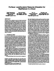
It turns out this problem can be converted to the well-known Linear Sum Assignment Problem (LSAP) [20] for which a couple of algorithms with polynomial-time complexity (e.g. Hungarian algorithm) have been proposed. A brief description of LSAP is included below. From the description, we can see LSAP requires the cost matrix be square, which implies LSAP can be directly applied to our problem only when the numbers of tasks and idle slots are equal. For the cases where they are not equal, we expand the cost matrix to a square one by adding extra rows or columns. If |T| is less than |IS|, we create |IS|-|T| dummy tasks whose assignment costs are 0 no matter where they are assigned. Figure 2 shows an example in which ti and sj represent tasks and idle slots respectively. The first |T| rows are from the original matrix and the last |IS|-|T| rows are for dummy tasks and all filled with 0. After this transformation, the original |T| x |IS| matrix is
expanded to a |IS| x |IS| square matrix and existing LSAP algorithms can be applied to find the optimal assignment of all |IS| tasks. After filtering out the dummy tasks from the solution given by LSAP, we obtain a valid assignment φ (termed φ-lsap). Given the fact that any valid LSAP algorithm guarantees an optimal solution for the expanded square matrix, we need to prove that φlsap is a solution to (3). Linear Sum Assignment Problem: Given n items and n workers, the assignment of an item to a worker incurs a known cost. Each item is assigned to one worker and each worker has one item assigned. Find the assignment that minimizes the sum of cost. Proof: We assume φ-lsap is not optimal and the optimal assignment is φ-opt. Apparently Csum(φ-opt) is less than Csum(φlsap). We expand the matrix to a square one and extend both φlsap and φ-opt to include the newly added dummy tasks. The key point is that the sum of the assignment costs of dummy tasks is always 0 regardless of where they are assigned. So the total assignment costs of φ-opt and φ-lsap do not change. As Csum(φopt) is less than Csum(φ-lsap), we find an assignment that yields lower cost sum than the solution given by LSAP algorithms. This contradicts with the assumption that LSAP algorithms guarantee optimal solutions. □ s1 t1 1 … … tT 0 tT+1 0 … 0 tIS 0
… … … … 0 0 0
sIS-1 4 … 2 0 0 0
(a) |T| < |IS|
sIS 0 … 3 0 0 0
s1 t1 2 t2 0 t3 5 t4 3 … … tT 0
... sIS sIS+1 … 1 0 … 0 0 … 2 0 … 5 0 … … 0
... 0 0 0 0 0
sT 0 0 0 0 0
…
0
0
2
0
(b) |T| > |IS|
Figure 2. Expand cost matrix to make it square. For (a), last |IS|-|T| rows are for dummy tasks we make up and all filled with 0. For (b), last |T|-|IS| columns are for dummy slots we make up and filled with 0.
From the proof above, we can see that any constant can be used to fill the extra rows without violating the optimality. The intuitive explanation is that the assignment of dummy tasks adds a constant value to the overall cost and does not change the (non-)optimality of each potential solution. Only the assignment of original tasks determines optimal solutions uniquely. For the case where |T| is larger than |IS|, the original matrix can be expanded to a |T| x |T| square matrix by adding |T|-|IS| extra columns that are filled with constant 0 (shown in Figure 2(b)). In other words, we create |T|-|IS| dummy slots. After applying any LSAP algorithm, we get the assignment of all |T| tasks. However, some tasks are assigned to dummy slots that do not exist in reality. After filtering out those invalid assignments, we obtain the final task assignment. The optimality of this approach can be proved similarly. From (1), we can see the accuracy of pairwise bandwidth information impacts the calculation of assignment costs. Ideally real-time network throughput information should be used. Network Weather Service [21] can be utilized to monitor and predict network usage without injecting an overwhelming number of probing packets. Based on above discussion, we first discuss below lsap-sched, which was introduced in [14]. The critical difference is network
bandwidth information is used to compute assignment costs while constant values were specified in [14]. Optimal data locality is guaranteed by lsap-sched. Algorithm skeleton of lsap-sched Input: instant system state Output: assignment of tasks to idle map slots Algorithm: TS ← the set of unscheduled tasks ISS ← the set of idle map slots C ← empty |TS| x |ISS| matrix for i in 1:|TS| for j in 1:|ISS| set C[i][j] according to (1) expandToSquare(C, 0) # expand to a square matrix R = lsap(C) # solve it using LSAP R = filterDummy(R) # filter out dummy tasks return R
Generally, the more idle slots and tasks there are, the more lsapsched outperforms dl-sched. The real cluster traces show the maximum utilization is seldom reached. CPU utilization was only 10% in Yahoo’s M45 cluster [22] and below 50% mostly in a Google cluster [23]. So on average a significant portion of slots is available when new tasks are submitted and lsap-sched is expected to perform substantially better than dl-sched. For the extreme case where a cluster operates near its maximum capacity, the performance advantage of lsap-sched is attenuated if new tasks are scheduled immediately. Instead, scheduling can be delayed by a short period to accumulate a sufficient number of idle slots before lsap-sched is applied. As our experiments below illustrate, the ratio of idle slots does not need to be high for lsapsched to yield significant performance improvement. For typical MapReduce clusters where most jobs are small, scheduling delay of several seconds is sufficient to generate performance boost.
3.3 Integration of Fairness We next investigate the integration of fairness into lsap-sched. Both capacity scheduler [5] and fair scheduler [6] take the same approach that jobs are organized into different groups by appropriate criteria (e.g. user-based, domain-based, pool-based). This approach is adopted by us as well. We do not enforce strict fairness which constrains each group cannot use more than its ration strictly, because it results in the waste of resources. We loosen the constraint. If there are excess idle slots to run all tasks, we just schedule them immediately to make full use of all resources even if some of the groups have used up their rations. If idle slots are insufficient, we need to selectively run tasks aiming to comply with ration specifications. We enhance lsap-sched to support fairness by carefully tuning the cost matrix C. The assignment cost of a task can be positively related to the resource usage of the group the task belongs to. In other words, for groups that use up or overuse the allocated capacity, their tasks have high assignment costs so that the scheduler does not favor them. Oppositely, the assignment costs of tasks from groups which underuse their allocated capacity are low so that they get higher priority. Let G represent the set of groups that a system administrator configures for a cluster, and i-th group is Gi. Each group contains some number of tasks and each task can only belong to exactly one group. Given a task T, function group(T) returns the group which T belongs to. Each group is assigned a weight/ration w which is the portion of map slots allocated to it. The sum of the weights of all groups is 1.0, which is formulated in (4). At time t,
rti(t) is the number of running tasks belonging to group Gi. Formula (5) calculates the ratio of map slots used by group Gi among all occupied map slots, which measures the real resource usage ratio of each group. For group Gi, the desired case is that si and wi are equal, which implies real resource usage exactly matches the configured share. If si is less than wi, group Gi can have more tasks scheduled immediately. If group Gi has used its entire ration, to schedule more tasks, it needs to wait until some of its tasks complete or there are sufficient idle slots to run all tasks. A Group Fairness Cost GFC is associated with each group to measure its “priority” of scheduling and calculated via (6). Groups with low GFC have high priority so that their tasks are considered before the tasks from groups with high GFC. Data locality sometimes conflicts with fairness. For example, it is possible that the unscheduled tasks that can achieve data locality are mostly from groups that have already used up their rations. And thus we get into the dilemma that tradeoffs between fairness and data locality must be made. To integrate data locality and fairness, we divide assignment cost into two parts: Fairness Cost (FC) and Data Locality Cost (DLC) (shown in (7)). From the aspect of fairness constraints, FC implies the order of tasks to be scheduled, and tasks with low FC should be scheduled before tasks with high FC. The range of FC is denoted by [0, FCmax]. DLC reflects the overhead of data movement and has the same meaning as the cost definition described above in section 3.2. The weights of FC and DLC can be implicitly adjusted by carefully choosing the value ranges. Table 1 gives examples of how fairness-favored scheduling, data locality-favored scheduling and both-favored scheduling can be achieved. The range of FC is [0, 100] for all the examples, while that of DLC varies. DLC with range [0, 20] makes the scheduler favor fairness because FC has a larger impact on the total assignment cost. DLC with range [0, 200] makes the scheduler favor data locality because the loss of data locality bumps up the total assignment cost significantly. DLC with range [0, 100] makes the scheduler favor both fairness and data locality, because the loss of data locality and fairness impacts overall assignment costs to the same extent. Above example shows how data locality and fairness can be balanced. We need to quantitatively determine the FC and DLC of tasks dynamically. Formula (8) shows how to calculate DLC, in which α is a configuration parameter fed by system administrators and implicitly controls the relative weight of DLC. If α is small, FC is dominant and the scheduler favors fairness. If α is large, DLC stands out and the scheduler favors data locality. If α is medium, FC and DLC become equally important. The calculation of FC is trickier and more subtle. As we mentioned, a GFC is associated with each group. One simple and intuitive strategy is for each group the FC of all its unscheduled tasks is set to its GFC. This implies all unscheduled tasks of a group have identical FC, and thus the scheduler is inclined to schedule all or none of them. Consider the scenario where FC dominates. Initially a group Gi underuses its ration just a little and has many unscheduled tasks. If group Gi has the lowest GFC, all its tasks naturally have the lowest FC and are scheduled to run before Table 1. Examples of How Tradeoffs are Made Fairness-favored
Data Locality-favored
FC*
DLC*
FC
DLC
[0, 100]
[0, 20]
[0,100]
[0,200]
Both-favored
FC
DLC
[0,100] [0,100]
* FC: fairness cost; DLC: data locality cost
other tasks so that group Gi uses significantly more resources. After scheduling, the resource usage of group Gi changes from slight underuse to heavy overuse. The reason why resource usage oscillates between underuse and overuse is the tasks in each group, no matter how many there are, are assigned the same FC. Instead, for each group we calculate how many of its unscheduled tasks should be scheduled based on the number of idle slots and its current resource consumption, and set only their FC to GFC. In (9) AS is the total number of all slots and AS·wi is the number of map slots that should be used by group Gi. Group Gi already has rti tasks running so we have AS·wi-rti slots at disposal (termed sto – Slots To Occupy). Because Gi can use only stoi more slots, accordingly the FC of at most stoi tasks is set to GFCi and that of other tasks is set to a larger value (1-wi)·β (β is the scaling factor of FC). So the tasks of each group do not always have the same FC. The number of unscheduled tasks for group Gi is denoted by uti. If uti is greater than stoi, we need to decide how to select stoi tasks out of uti tasks. Then data locality comes into play, and the tasks that can potentially achieve data locality are chosen. Details are given in the proposed algorithm below. Note parameters α and β, which are used to balance data locality and fairness, are specified by system owners based on their performance requirement and desired degrees of fairness.
si (t ) =
|G| i =1
wi = 1 (0 < wi ≤ 1)
rti (t ) |G | rt (t ) j =1 j
GFCi =
(1 ≤ i ≤ G )
si ⋅100 wi
Cij = FC (i, j ) + DLC (i, j ) if data locality is achieved 0 DS (Ti ) DLC (i, j ) = α ∗ otherwise max {BW ( ND (Ti , c), N ( S j ))} 1≤c ≤ Ri
(4) (5)
(6) (7)
(8)
stoi = max(0, AS ⋅ wi − rti ) (9) Based on above discussion, scheduling algorithm lsap-fairsched is proposed and shown below. The main difference than lsap-sched is how assignment costs are calculated. Lines 7-8 find the set of nodes with idle slots. Lines 10-12 find the set of tasks whose input data are stored on nodes with idle slots. So these tasks have the potential to achieve data locality while all other tasks will lose data locality definitely for current scheduling. Lines 13-16 calculate sto of all groups. Lines 18-27 calculate task FC. Lines 29-33 calculate DLC. Line 35 adds together matrices FC and DLC to form the final cost matrix, which is expanded to a square matrix shown in line 36. After that, a LSAP algorithm is used to find the optimal assignment which is subsequently filtered and returned. Algorithm skeleton of lsap-fair-sched Input: α: DLC scaling factor for non data local tasks β: FC scaling factor for tasks that are beyond its group allocation Output: assignment of tasks to idle map slots Functions:
rt(g): return a set of running tasks that belong to group g. node(s): return the node where slot s resides reside(T): returns a set of nodes that host the input data of task T Algorithm: 1 TS ← the set of unscheduled tasks 2 ISS ← the set of idle map slots 3 w ← rations/weights of all groups 4 ut ← the number of unshed. tasks for all groups 5 gfc ← GFC of all groups calculated via (6) 6 INS ← ∅ # the set of nodes with idle slots 7 for slot in ISS: 8 INS ← INS ⋃ node(slot) 9 # tasks that can potentially gain data locality DLT[1:|G|] = ∅ 10 for T in TS: 11 if reside(T) ∩ INS ≠ ∅: 12 DLT[group(T)] = DLT[group(T)] ⋃ T 13 for i in 1:|G| 14 diff = w[i] · AS - rt[i] 15 if diff > 0: sto[i] = min(diff, ut[i]) 16 else: sto[i] = 0 17 18 fc[1:|TS|][1:|ISS|] = 0 #fill with deft value 19 for i in 1:|G| 20 tasks = G[i] #a list of tasks in group i 21 NDLT = tasks - DLT[i] #non-local tasks 22 fc[tasks] = β·(1-w[i]) #default value 23 if |DLT[i]| ≥ sto[i]: 24 tasks = DLT[i][1:sto[i]] #choose a subset 25 else if ut[i] > sto[i]: 26 tasks = DLT[i] ⋃ NDLT[1:(sto[i]-|DLT[i]|]] 27 fc[tasks] = gfc[i] #assign GFC to some tasks 28 29 dlc[1:|TS|][1:|ISS|]=1 30 for T in ⋃DLT[i]: 31 for j in 1:|ISS| 32 if co-locate(T, ISS[j]): dlc[T][j] = 0 33 else: dlc[T][j]= α·DS(T)/BW(T,ISS[j]) 34 35 C = fc + dlc 36 if C is not square: expandToSquare(C, 0) 37 R = lsap(C) 38 R = filterDummy(R) 39 return R
In above strategy, some tasks may get starved although the possibility is remote (e.g. tasks with bad data locality may be queued indefinitely). FC and DLC can be reduced for the tasks that have been waiting in queue for long time, so that they tend to be scheduled at the subsequent scheduling points.
4. EXPERIMENTS In the experiments below, the main considered system factors include the number of nodes, the number of slots per node, the ratio of idle slots, and replication factor. One factor is varied while others are fixed in each test. We have conducted simulation experiments to evaluate the effectiveness of our proposed algorithms. We are preparing FutureGrid to support direct evaluation. Because we do not have access to real MapReduce production clusters, we need to mimic multi-user mode by setting some factors artificially (such as slot utilization, workload, and bandwidth usage). We expect to have FutureGrid results to add to published paper if accepted.
4.1 Overhead of LSAP Solver We measured the time taken by lsap-sched to compute optimal task assignment in order to understand the overhead of solving LSAP. We varied the number of tasks from 100 to 3000 with step size 400, and the number of idle slots was equal to the number of tasks for each test. They represent small-sized to moderate-sized
clusters. The corresponding cost matrices were constructed and fed into LSAP solver. It took 7ms, 130ms, 450ms, and 1s for the LSAP solver to find optimal solutions given the matrices of sizes 100x100, 500x500, 1700x1700 and 2900x2900. So the overhead is acceptable in small-sized to medium-sized clusters. Note in our tests, values in the matrices were randomly generated, which eliminates the possibility to mine and explore useful patterns of cost distribution. In reality, the cost of data movement exhibits locality for typical hierarchical network topologies, which can be used to speed up the execution potentially.
4.2 Improvement of Data Locality In this test, we evaluate how lsap-sched impacts the percent of data local tasks. In the simulated system, the number of nodes varied from 100 to 500 with step size 50, and each node had 4 slots. Replication factor was 3. The ratio of idle slots was fixed to 0.5 and enough tasks were generated to utilize all idle slots. The results are shown in Figure 3. Figure 3(a) shows the goodness of data locality for dl-shed and lsap-sched. Obviously, the goodness of data locality is pretty stable for both algorithms: dl-sched achieves 83% while lsap-sched achieves 97%. Their differences are shown in Figure 3(b), which implies lsap-sched increases the goodness of data locality by 12% - 14%. This indicates that lsap-sched consistently outperforms dl-sched significantly when the system is scaled out. In addition, we observe that the improvement oscillates in Figure 3(b). Our conjecture of the cause is that the number of all possible data and slot distributions is gigantic and only a portion of them was covered in our tests. Then we varied replication factor from 1 to 19 and fixed the number of nodes to 100. The goodness of data locality was measured and is shown in Figure 4(a). The increase of replication factor yields substantial data locality improvement for both lsapsched and dl-sched; and lsap-sched can more efficiently explore the increasing data redundancy and thus achieve better data locality. Common replication factors 3 and 5 yield surprisingly high data locality 72% and 88% respectively for lsap-sched. Finally, we set the total number of idle slots to 100 and increased the number of tasks from 5 to 100 so that they used more and more idle slots. Results are shown in Figure 4(b). Data locality degrades slowly as more tasks are injected into the system, and the degradation of lsap-sched is much less severe than that of dlsched. When the number of tasks is much smaller than that of idle slots, the scheduler has the great freedom of picking the best slots to assign tasks. As their numbers become close, more tasks need to be scheduled in one “wave” and the cherry-picking freedom is gradually attenuated. This explains why the increase of the number of tasks has negative impact on data locality.
4.3 Reduction of Data Locality Cost In above tests, we measured the percentage of data local tasks. In
(a) Data locality of dl-sched and lsap-sched (b) Percent of improvement
Figure 3. Comparison of data locality (varied # of nodes)
(a) Varied replication factor
(b) Varied the number of tasks
Figure 4. Comparison of data locality (varied rep. factor and # of tasks) reality, performance depends upon not only the goodness of data locality, but also the incurred data movement penalty of non data local tasks. In this test, we measure the overall data locality cost (DLC) to quantify the performance degradation brought by non data local tasks. The DLC of any non data local task was set to 1 regardless of the proximity between the location of compute and input data, which assumes that the cluster is homogeneous. The same test environment as above is used. Figure 5(a) shows the absolute DLC. As the number of nodes is increased, the DLC of dl-sched increases much faster than that of lsap-sched. So lsapsched is more resilient to system scale-out than dl-sched. We also computed the DLC reduction of lsap-sched against dl-sched, and show results in Figure 5(b). We observe that lsap-sched eliminates 70% - 90% of the DLC of dl-sched.
(a)Overall DLC of dl-sched and lsap-sched(b)Reduction of DLC(in percent)
Figure 5. Comparison of data locality cost (with equal net. bw.) Previously, constant value 1 was used as the DLC of non data local tasks, which does not reflect the fact that pairwise network bandwidths are not uniform (e.g. intra-rack throughput is usually higher than cross-rack throughput). In this test, we complicate the tests by setting non-constant costs. We simulated a cluster where each rack has 20 nodes. Again the DLC of data local tasks is 0. The DLC of rack local tasks (i.e. computation and input data are co-located on the same rack) follows a Gaussian distribution with mean and standard deviation being 1.0 and 0.5 respectively. The DLC of remote tasks follows another Gaussian distribution with mean and standard deviation being 4.0 and 2.0 respectively. This setting matches the reality that cross-rack data fetching incurs higher cost than intra-rack data fetching. We varied the total number of nodes from 100 to 500 and measured DLC. Firstly the ratio of idle slots was set to 50% and DLC is shown in Figure 6. Lsap-sched still outperforms dl-sched significantly by up to 95%. By comparing Figure 5 and Figure 6, we observe that rack topology does not result in performance degradation. Dl-sched is rack aware in the sense that rack local tasks are preferred over remote tasks if there are no node local tasks. So it avoids assigning tasks to the nodes where they need to fetch input data from other racks with best efforts. Lsap-sched is naturally rack aware because the high cross-rack data movement cost prohibits non-optimal task assignments. So both dl-sched and lsap-sched can effectively utilize the network topology information. Then we decreased the ratio of idle slots from 50% to 20%, which
implies there was a fewer number of idle slots. Results are show in Figure 7. Compared with Figure 6, the DLC of dl-sched is decreased and the DLC of lsap-sched is increased, so that the performance superiority of lsap-sched over dl-sched becomes less significant which is between 60% and 70%. When there are only a small number of idle slots, the room of improvement brought by lsap-sched is minor. For the extreme case where there is only one idle slot, dl-sched and lsap-sched becomes equivalent approximately. The more available resources and tasks there are, the more lsap-sched reduces DLC. The utilization of typical production clusters rarely reaches up to 80% [22, 23]. So we believe lsap-sched can offer substantial benefit in moderatelyloaded clusters. Then we fixed the number of nodes to 100 and increased replication factor from 1 to 13 with step size 2. The other settings were identical to the test above except each node has 1 idle slot. As replication factor is increased, we expect positive impact on DLC because the possibility of achieving better data locality increases theoretically. Test results are shown in Figure 8. Firstly, DLC drastically decreases as replication factor is increased initially from small values, and the decrement of DLC becomes less significant as replication factor gets larger and larger. Secondly, when replication factor is 1, lsap-sched and dlsched perform comparably. Lsap-sched has much faster DLC decrease than dl-sched as replication factor grows, and it almost thoroughly eliminates DLC when replication factor is larger than 7. Figure 8(b) shows a low replication factor (e.g. 3) is sufficient for lsap-sched to outperform dl-sched by over 50%. Note the number of slots per node was set to 1 in this test, and increasing it can bring larger improvement.
(a)Overall DLC of dl-sched and lsap-sched(b)Reduction of DLC(in percent)
Figure 6. Comparison of DLC with 50% idle slots (rack aware)
(a)Overall DLC of dl-sched and lsap-sched(b)Reduction of DLC(in percent)
Figure 7. Comparison of DLC with 20% idle slots (rack aware)
4.4 Evaluation of lsap-fair-shed We have shown that theoretically fairness and data locality can be integrated together by carefully setting Fairness Cost and Data Locality Cost. In this experiment, we conducted a series of simulations to evaluate our proposed algorithm lsap-fair-sched. For each group, formula (10) calculates the fairness distance between the actual resource allocation si and the desired allocation specified via weights wi. Value 0 indicates that the group uses exactly its ration. If its value is greater than 0, the
(a)Overall DLC of dl-sched and lsap-sched(b)Reduction of DLC(in percent)
Figure 8. Comparison of DLC w/ rep. factor varied (rack aware) resource usage of the group either exceeds or is less than its ration. So its value indicates the compliance with administratorprovided allocation policies, and smaller is better usually. Formula (11) calculates the mean of fairness distance of all groups and serves as a metric to measure the fairness of resource allocation. At initial time instant 0, the fairness distance is denoted by d(0). Then submitted tasks are scheduled, and at time t the fairness distance becomes d(t). If the scheduler is fairnessaware, usually d(t) should be smaller than d(0) which implies fairness is improved. Given an initial state, we use d(0)-d(t) to measure to what extent lsap-fair-sched improves fairness, and larger is better.
di (t ) = | si (t ) − wi | / wi
(10)
(11)
d (t ) =
|G |
d (t ) i =1 i G
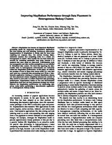
In our tests, there were 60 nodes; each node had 1 slot; half of all slots were idle; replication factor was 1; and there were 30 running tasks and 90 tasks to schedule. In addition, there were 5 groups to which tasks belong. Weights for groups were {20, 21, 22, 23, 24} and normalized to {20/31, 21/31, 22/31, 23/31, 24/31} so that they add up to 1.0. The groups to which running tasks belong were randomly assigned. The DLC of non-local tasks was varied and results are shown in Figure 9. Initially, DLC is small compared with FC so that FC dominates the total assignment cost and lsap-fair-sched improves fairness most. Gradually, as the DLC of non-local tasks increases, data locality gains larger weight so that data locality improves and fairness deteriorates. After the DLC of non-local tasks gets sufficiently large, data locality becomes the dominant factor so that scheduling favors data locality mainly. Another observation is that improvement/ deterioration of data locality/fairness is not smooth, and the curves are staircase shaped. During the continuous increase of DLC, not every small increment makes DLC become dominant. There are some critical steps that cause “phase transition” and make the assignment costs of some tasks become larger than that of other tasks that had larger cost before, so that data locality becomes dominant in scheduling. Oppositely, the non-critical increase is not sufficient to influence scheduling decisions.
5. CONCLUSIONS In this paper, we conducted an in-depth investigation of data locality and fairness in MapReduce. We illustrated the default Hadoop scheduling strategy dl-sched does not guarantee optimal data locality. Then we used a cost matrix to represent the associated data movement costs of all {task, slot} pairs, and reformulated the scheduling problem into a new problem that tries to find an assignment that minimizes the sum of assignment cost. We proposed augmented lsap-sched that gives optimal data locality by utilizing the well-known problem LSAP. The
Intensive Applications. In Proc. of HPDC'02. IEEE Computer Society, Washington, DC, USA, 352-. [8] H. H. Mohamed and D. H. J. Epema. 2004. An evaluation of the close-to-files processor and data co-allocation policy in multiclusters. In Proc. of CLUSTER'04. IEEE Computer Society, Washington, DC, USA, 287-298. [9] R. Chang, J. Chang, and S. Lin. 2007. Job scheduling and data replication on data grids. Future Gener. Comput. Syst. 23, 7 (August 2007), 846-860. Figure 9. Tradeoffs between fairness and data locality conducted simulation shows lsap-sched can improve the goodness of data locality and reduce the overall DLC substantially. In addition, we investigated fairness and noticed the conflict between fairness and data locality. The assignment cost is split into two parts: fairness cost and data locality cost. We enhanced lsap-sched to balance fairness and data locality based on the userprovided weights. Corresponding experiments show that the relative importance of fairness and data locality can be tuned effectively and conveniently. The desired setting is system specific and depends upon fairness requirements and the typical workload of submitted MapReduce jobs. We are implementing our algorithms in Hadoop and expecting to get real results later that will be added to this paper if accepted.
6. ACKNOWLEDGMENTS This material is based upon work supported in part by the National Science Foundation under Grant No. 0910812 to Indiana University for "FutureGrid: An Experimental, High-Performance Grid Test-bed." Partners in the FutureGrid project include U. Chicago, U. Florida, San Diego Supercomputer Center - UC San Diego, U. Southern California, U. Texas at Austin, U. Tennessee at Knoxville, U. of Virginia, Purdue U., and T-U. Dresden.
7. REFERENCES [1] J. Dean and S. Ghemawat. 2008. MapReduce: simplified data processing on large clusters. Commun. ACM 51, 1 (January 2008), 107-113. [2] Yahoo! Launches World’s Largest Hadoop Production Application, Yahoo! Developer Network, http://developer.yahoo.com/blogs/hadoop/2008/02/yahooworlds-largest-production-hadoop.html [3] J. Lin and C. Dyer. 2009. Data-intensive text processing with MapReduce. In Proc. of HLT-NAACL (Tutorial Abstracts)'2009. pp.1~2 [4] X. Qiu, J. Ekanayake, S. Beason, T. Gunarathne, G. Fox, R. Barga, and D. Gannon. 2009. Cloud technologies for bioinformatics applications. In Proc. of workshop MTAGS '09. ACM, New York, NY, USA [5] Hadoop’s Capacity Scheduler http://hadoop.apache.org/core/docs/current/capacity_schedul er.html.
[10] K. Ranganathan and I. T. Foster. 2001. Identifying dynamic replication strategies for a High-Performance data grid. In Proc. of GRID’01. London, UK: Springer-Verlag, pp. 75-86. [11] M. Zaharia, D. Borthakur, J. Sarma, K. Elmeleegy, S. Shenker, and I. Stoica. 2010. Delay scheduling: a simple technique for achieving locality and fairness in cluster scheduling. In Proc. of EuroSys '10. ACM, New York, NY, USA, 265-278 [12] B. Palanisamy, A. Singh, L. Liu, and B. Jain. 2011. Purlieus: locality-aware resource allocation for MapReduce in a cloud. In Proc. of SC’11. ACM, New York, NY, USA [13] M. Zaharia, A. Konwinski, A. D. Joseph, R. Katz, and I. Stoica. 2008. Improving MapReduce performance in heterogeneous environments. In Proc. of OSDI'08. USENIX Association, Berkeley, CA, USA, 29-42. [14] Z. Guo, G. Fox, and M. Zhou. 2012. Investigation of Data Locality in MapReduce. In Proc. of CCGrid’12. To appear. [15] P. Agrawal, D. Kifer, and C. Olston. 2008. Scheduling shared scans of large data files. In Proc. of VLDB Endow., vol. 1, no. 1, pp. 958-969, Aug. 2008. [16] A. Ghodsi, M. Zaharia, B. Hindman, A. Konwinski, S. Shenker, and I. Stoica. 2011. Dominant resource fairness: fair allocation of multiple resource types. In Proc. of NSDI'11 [17] M. Isard, V. Prabhakaran, J. Currey, U. Wieder, K. Talwar, and A. Goldberg. 2009. Quincy: fair scheduling for distributed computing clusters. In Proc. of SOSP’09 [18] B. Schroeder and M. Harchol-Balter. 2000. Evaluation of Task Assignment Policies for Supercomputing Servers: The Case for Load Unbalancing and Fairness. In Proc. of HPDC '00 [19] S. Ghemawat, H. Gobioff, and S. Leung. 2003. The Google file system. In Proc. of SOSP '03. ACM, New York, NY, USA, 29-43. [20] R.E. Burkard, M. Dell'Amico, and S. Martello. 2009. Assignment problems. SIAM, Society for Industrial and Applied Mathematics [21] R. Wolski, N. Spring, and J. Hayes. 1999. The network weather service: a distributed resource performance forecasting service for metacomputing. Future Gener. Comput. Syst. 15, 5-6 (October 1999), 757-768
[6] Matei Zaharia, “The Hadoop Fair Scheduler” http://developer.yahoo.net/blogs/hadoop/FairSharePres.ppt
[22] S. Kavulya, J. Tan, R. Gandhi, and P. Narasimhan. 2010. An Analysis of Traces from a Production MapReduce Cluster. In Proc. of CCGRID '10
[7] K. Ranganathan and I. Foster. 2002. Decoupling Computation and Data Scheduling in Distributed Data-
[23] L. A. Barroso and U. H. Olzle. 2007. The case for energyproportional computing. Computer , vol.40, no.12, pp.33-37