stiffness (hence less welding spots), than the optimal decomposition with the typical joint rates available in the .... spring constants of torsional springs Nm/rad of the joint cor- responding to .... case studies, the rates of the torsional springs at each joint in a ..... value T is 3750 â Nmâ¡ assuming the static wheel reaction in the.
Decomposition-Based Assembly Synthesis for Structural Stiffness Naesung Lyu Kazuhiro Saitou e-mail: 兵nlyu,kazu其@umich.edu Department of Mechanical Engineering, University of Michigan, Ann Arbor, MI
1
This paper presents a method that systematically decomposes product geometry into a set of components considering the structural stiffness of the end product. A structure is represented as a graph of its topology, and the optimal decomposition is obtained by combining FEM analyses with a Genetic Algorithm. As the first case study, the side frame of a passenger car is decomposed for the minimum distortion of the front door panel geometry. As the second case study, the under body frame of a passenger car is decomposed for the minimum frame distortion. In both case studies, spot-weld joints are considered as joining methods, where each joint, which may contain multiple weld spots, is modeled as a torsional spring. First, the rates of the torsional springs are treated as constant values obtained in the literature. Second, they are treated as design variables within realistic bounds. By allowing the change in the joint rates, it is demonstrated that the optimal decomposition can achieve the smaller distortion with less amount of joint stiffness (hence less welding spots), than the optimal decomposition with the typical joint rates available in the literature. 关DOI: 10.1115/1.1582879兴
Introduction
To design any structural product, engineers adopt one of the two design methods: top-down and bottom-up methods. As the end products become more complicated and highly integrated, the top-down method is preferred since it allows the easier design assessment of an entire product during the design process. Topdown methods typically start with the preliminary design of the overall end product structure and proceed with the detailed design of components and substructures. If geometries and desired functions are simple, the structure can be built in one piece. To build complex structures in one piece, however, engineers need sophisticated manufacturing methods that would likely result in the higher manufacturing cost. Also, one piece structure will suffer from the lack of modularity: it would require the change or replacement of the entire structure even for local design changes or failures. It would be often natural, therefore, to design a structural product as an assembly of components with simpler geometries. To design multi-component structural products in top-down fashion, an overall product geometry must be decomposed at some point during the design process. In industry, such decompositions are typically done prior to the detailed design of individual components, taking into account of geometry, functionality, and manufacturability issues. However, this process is usually nonsystematic and hence might result in a decomposition overlooking the integrity of the end product. For instance, automotive industry utilizes a handful of basic decomposition schemes of a vehicle that have not been changed for decades. This is because the desired form, functionality, materials, joining methods, and weight distribution of mass-production vehicles have not changed much for decades. However, the conventional decomposition schemes may no longer be valid for the vehicles with new technologies such as space frame, lightweight materials, and fuel cell or battery powered motors, which would have dramatically different structural properties, weight distribution, and packaging requirements. This motivates the development of a systematic decomposition methodology presented in this paper. In our previous work 关1–3兴, we have termed assembly synthesis as the decision of which component set can achieve a desired function of the end product when assembled together, and assembly synthesis is achieved by the decomposition of product geomContributed by the Reliability, Stress Analysis, and Failure Prevention Committee for publication in the JOURNAL OF MECHANICAL DESIGN. Manuscript received May 2002; rev. Nov. 2002. Associate Editor: J. Moosbrugger.
452 Õ Vol. 125, SEPTEMBER 2003
etry. Since assembly process generally accounts for more than 50% of manufacturing costs and also affects the product quality 关4兴, assembly synthesis would have a large impact on the quality and cost of the end product. As an extension of our previous work, this paper introduces a method for decomposing a product geometry considering the structural stiffness of the end product. Because decomposition will determine the location of the joints between components, the structural integrity 共e.g., stiffness兲 of the end-product will be heavily influenced by the choice of a particular decomposition. Designers can use this method to get feedback on the possible decompositions before the detailed design stage. Via the decomposition of a graph representing its topology, a product is decomposed into a candidate set of components with simpler geometries, where joints among components are modeled as torsional springs. By combining FEM analyses with Genetic Algorithms 关5,6兴, the optimal decomposition that gives the desired structural property of the end product is obtained. The case studies discuss the assembly synthesis of the side door panels 共Case Study 1兲 and under body frame of a passenger car 共Case Study 2兲.
2
Related Work
2.1 Design for Assembly and Assembly Sequence Design. Many attempts have been made on assembly design and planning for decades. Among them, Boothroyd and Dewhurst 关7兴 are widely regarded as major contributors in the formalization of design for assembly 共DFA兲 concept. In their method 关8兴, assembly costs are first reduced by the reduction of part count, followed by the local design changes of the remaining parts to enhance their assembleability and manufacturability. This basic approach is adopted by most subsequent works on DFA. There are a number of researchers investigating the integration of DFA and assembly sequence planning 关9,10兴, where assembly sequence planning is proposed as the enumeration of geometrically feasible cut-sets of a liaison graph, an undirected graph representing the connectivity among components in an assembly. The local design changes are made to the components to improve the quality of the best assembly sequence. These works, however, focus on the local design changes of a given assembly design 共i.e., already ‘‘decomposed’’ product design兲, and have less emphasis on how to synthesize an assembly to start with. 2.2 Automotive Body Structure Modeling. In automotive body structure, high stiffness is one of the most important design
Copyright © 2003 by ASME
Transactions of the ASME
Fig. 2 Example decompositions of a graph and the corresponding values of vector x . „a… the original graph with x Ä„1,1,1…, and „b… two component decomposition with x Ä„0,0,1….
variable x i can be used to represent a decomposition of structural topology graph G. The dimension of the vector x⫽(x i ) is equal to the number of the edges 兩 E 兩 in G: Fig. 1 Outline of the decomposition procedure. „a… structure to be decomposed, „b… basic members and potential joint locations, „c… structural topology graph G , „d… optimal decomposition of G , and „e… resulting decomposition of the original structure.
factors, since it is directly related the improved ride and NVH 共Noise, Vibration, and Harshness兲 qualities and crashworthiness 关11兴. To accurately predict the stiffness of an assembled body structure, Chang 关12兴 used a beam-spring model of BIW where spot-welded joints were modeled as torsional springs. In this work he demonstrated that the model can accurately predict the global deformation of automotive body substructures. Recently, correlation between torsional spring properties of joints and the length of structural member was studied 关13兴 to assess the accuracy of joint model. Kim 关14兴 employed an 8-DOF beam theory for modeling joints to consider the warping and distortion in vibration analysis. However, these works focus on the accurate prediction of the structural behavior of a given assembly 共i.e., already ‘‘decomposed’’ structure design兲 and do not address where to place joints based on the predicted stiffness of an assembly.
3
Approach
This section describes the proposed method for simultaneously identifying the optimal set of components and joint attributes 共rates of torsional springs兲 considering the stiffness of the assembled structure. It is assumed that joints have less stiffness than components and therefore reduce the rigidity of the overall structure.1 The following steps outline the basic procedure: 1. Given a structure of interest 共Fig. 1共a兲兲, define the basic members and potential joint locations 共Fig. 1共b兲兲. 2. Construct a structural topology graph G⫽(V,E) with node set V and edge set E, which represents the connectivity of the basic members defined in step 1 共Fig. 1共c兲兲. A node and an edge in G correspond to a member and a joint, respectively. 3. Obtain the optimal decomposition of G that gives the best structural performance via Genetic Algorithm 共Fig. 1共d兲兲, and map the decomposition result back to the original structure 共Fig. 1共e兲兲. During optimization, the structural performance of decomposition is evaluated by a Finite Element Method. 3.1 Definition of Design Variables. Since a graph can be decomposed by deleting some edges, a vector x⫽(x i ) of binary 1
While this is true for many joints such as spot welds, threaded fasteners, and rivets, some joints 共e.g., arc welds兲 can be stiffer than components themselves.
Journal of Mechanical Design
x⫽ 共 x 1 x 2 . . . x 1 . . . x 兩 E 兩 ⫺1 x 兩 E 兩 兲 where x i⫽
再
1 0
(1)
if e i exists in the decomposed graph otherwise
Figure 2 illustrates example decompositions of a graph and the corresponding values of vector x. Figure 2共a兲 shows the original graph G without decomposition, where V⫽ 兵 n 1 ,n 2 ,n 3 其 and E ⫽ 兵 e 1 ,e 2 ,e 3 其 . Since all edges are present without decomposition, the corresponding vector x⫽(x 1 ,x 2 ,x 3 ) is 共1,1,1兲. If vector x takes this value, an entire graph G is interpreted as one component, which is denoted as C 1 in the figure. Similarly, Fig. 2共b兲 shows a two-component decomposition consisting of components C 1 and C 2 obtained by deleting e 1 and e 2 共indicated as dashed lines兲 in G. This decomposition can be represented using vector x as x⫽(x 1 ,x 2 ,x 3 )⫽(0,0,1). Joint attributes are defined as another vector y ⫽(y1,y2, . . . ,y兩 E 兩 ), where y i , i⫽1,2, . . . , 兩 E 兩 is a n-dimensional vector representing the joint attributes of edge e i in the structural topology graph. In other words, the joint design at edge e i is determined by n design variables yi ⫽(y i1 ,y i2 , . . . ,y in ). In the following case studies, joint attribute y i represents the rates 共spring constants兲 of torsional springs 关Nm/rad兴 of the joint corresponding to edge e i of the structural topology graph. In the first case study, the 2-dimensional analysis model 共side frame decomposition of a passenger car兲 needs only one design variable 共rotation around z axis兲 for joint design. In this case n⫽1 and yi ⫽y i ⫽k iz . However, in the second case study 共under body frame decomposition of a passenger car兲 we considered 3-dimensional analysis model that requires three design variables 共rotations around spring x, y, and z axes兲 for joint design. In this case n ⫽3 and yi ⫽(k ix ,k iy ,k iz ). During optimization, the value of yi is only considered if x i ⫽0 when joint between components is required. 3.2 Definition of Constraints. The first constraint for the design variable x comes from the definition of x. Namely, each element of the vector x should be 0 or 1: x i 苸 兵 0,1其
(2)
In the current formulation, we assume a desired number of decomposition k is given by the designer, considering this is constrained by the number of available assembly stations.2 Therefore, the decomposition of G should result in k disconnected subgraphs: NគCOMPONENTS 共 GRAPH共 x兲兲 ⫽k
(3)
2 Given a cost model of component manufacturing, it would be possible to include k in the design variable and determine the optimal number of components, which is a part of future investigation.
SEPTEMBER 2003, Vol. 125 Õ 453
where GRAPH共x兲 is a function that returns the graph corresponding to the decomposition of G with x, and NគCOMPONENTS(G) is a function that returns the number of disconnected subgraphs 共‘‘components’’兲 in graph. The third constraint of x is to ensure the decomposed components are economically manufacturable by given manufacturing means. For example, components with a branched topology would not be economically manufacturable by sheet metal stamping. Also, when we consider 3D structure with stamping process, any decomposed component should be on 2 dimensional plane. Those constraints will be determined by the manufacturing methods and also by the capacity of the machines to be used. The following is a general form of manufacturability constraint: ISគMANUFACTURABLE 共 GRAPH 共 x兲兲 ⫽1
(4)
where ISគMANUFACTURABLE(G) is a function that returns 1 when all disconnected subgraphs in G are manufacturable by given manufacturing methods, such as stamping of sheet metal, and otherwise returns 0. In the following case studies, it is simply defined as the condition where the bounding boxes of all decomposed components are less than a given size, which represents the upper limit of stamping die size. Finally, elements of yi should simply be among the feasible selections: y i j 苸F
i⫽1,2, . . . , 兩 E 兩 ,
j⫽1,2, . . . ,n
(5)
where F is a set of feasible values of given joint attributes 共the rate of torsional spring in the following examples兲. Assuming that rate of a joint is defined by the type of the joint and the number of welding spots, the value of y i j is chosen among discrete values within the reasonable range of torsional spring rate. 3.3 Definition of Objective Function. A component set specified by vector x 共a set of the node sets of disconnected subgraphs in GRAPH 共x兲兲 is evaluated for the stiffness of the assembled structure with the joint attribute specified by y. The stiffness of an assembled structure can be measured as the negative of the sum of displacements at the pre-specified points of the structure for given boundary conditions: stiffness⫽⫺DISPLACEMENTS 共 GRAPH共 x兲 ,y兲
Fig. 3 Chromosome representation of design variables x Ä„ x i … and yÄ„ y i …, where the elements of these vectors are simply laid out to form a linear chromosome of length „1 ¿ n … * 円 E 円 . Note n is the number of design variables that determine the design of one joint.
(6)
where DISPLACEMENTS(G,y) is a function that returns the sum 共or the maximum兲 of displacements at the pre-specified points of the assembled structure, computed by finite element methods. Since we assume the number of components is given, a decomposition would be the stiffest if the maximum spring constant is used at all joints. This corresponds to the situation where the maximum number of spot welds is used for all joints, which is obviously not a very economical solution. It would be of engineering interest, therefore, to find out the optimal balance between the sum of spring constants 共a measure of the total number of spot welds兲 and structural stiffness of the assemble structure. This results in the following objective function 共to be maximized兲 that evaluates stiffness of the structure and also total sum of spring constants in the joints:
x⫽ 共 x i 兲 , y⫽ 共 yi 兲 ,
y i⫽共 y i j 兲,
x i 苸 兵 0,1其 , y i j 苸F,
i⫽1, . . . , 兩 E 兩 i⫽1, . . . , 兩 E 兩 ,
j⫽1, . . . ,n
It should be noted that the above optimization model contains a standard k-partitioning problem of an undirected graph 关14兴, and additional nonlinear terms in the objective functions and constraints. 3.4 Genetic Algorithms. Due to the NP-completeness of the underlying graph partitioning problem 关15兴, the above optimization model is solved using Genetic Algorithm 共GA兲. GA is a heuristic optimization algorithm that simulates the process of natural selection in biological evolution 关5,6兴. The results of the following examples are obtained using a steady-state GA 关16兴, a variation of the ‘‘vanilla’’ GA tailored to prevent premature convergence. Basic steps of a steady-state GA is outlined below 关2兴: 1. Randomly create a population P of n individuals with chromosomes 共a representation of design variable x兲. Evaluate their fitness values and store the best chromosome. Also create an empty subpopulation Q. 2. Select two chromosomes c i and c j in P with probability: Prob共 c i is selected兲 ⫽
fi 兺 fk
where f i is the fitness value of chromosome c i . 3. Crossover c i and c j to generate two new chromosomes c i⬘ and c ⬘j . 4. Mutate c i⬘ and c ⬘j with a certain low probability. 5. Evaluate the fitness values of c i⬘ and c ⬘j . Add them in Q. If Q contains less than m new chromosomes, go to step 2. 6. Replace m chromosomes in P with m chromosomes in Q. Empty Q. Update the best chromosome and increase the generation counter. If the generation counter has reached a pre-specified number, terminate the process and return the result. Otherwise go to step 2.
where C is a positive constant, stiffness is defined as Eq. 共6兲, w 1 and w 2 are positive weights. The purpose of constant C is to ensure the positive value of fitness for any values of x and y, required by Genetic Algorithms as stated below. After all, the following optimization model is to be solved: maximize f (x,y) 共objective function in Eq. 共7兲兲 subject to
In GAs, design variables are represented as a ‘‘string’’ of numbers called chromosomes on which genetic operators such as crossover and mutation are performed. The components of our two design variables x⫽(x i ) and y⫽(y i ) are simply laid out as x 1 ,x 2 , . . . , x 兩 E 兩 ,y 11 , y 12 , . . . , y 1n , y 21 ,y 22 , . . . , y 2n , . . . , y 兩 E 兩 1 , y 兩 E 兩 2 , . . . ,y 兩 E 兩 n in a linear chromosome of length (1⫹n) * 兩 E 兩 as illustrated in Fig. 3. Two-point crossover is used where the crossover sites are selected to ensure a cut in both x and y portions of the chromosome. Since we have formulated the optimization model as a maximization problem, the fitness values of a chromosome can be computed from the corresponding values of the design variables x and y as:
NគCOMPONENTS 共 GRAPH 共 x兲兲 ⫽k
fitness⫽ f 共 x,y兲 ⫺penalty
f 共 x,y 兲 ⫽C⫹w 1 •stiffness⫺w 2 •
兺y
ij
ISគMANUFACTURABLE 共 GRAPH 共 x兲兲 ⫽1, 454 Õ Vol. 125, SEPTEMBER 2003
(7)
(8)
where penalty is defined as: Transactions of the ASME
penalty⫽w 3 共 NគCOMPONENTS 共 GRAPH 共 x兲兲 ⫺k 兲 2 ⫹w 4 共 ISគMANUFACTURABLE 共 GRAPH 共 x兲兲 ⫺1 兲 2 (9) where w 3 , w 4 are positive weights. After all, the fitness function looks like: fitness⫽C⫺w 1 •DISPLACEMENTS 共 GRAPH 共 x兲 ,y兲 ⫺w 2 •
兺 y ⫺w 共 NគCOMPONENTS 共 GRAPH 共 x兲兲 ⫺k 兲 i
3
2
⫺w 4 共 ISគMANUFACTURABLE 共 GRAPH 共 x兲兲 ⫺1 兲 2 (10) As stated earlier, computing DISPLACEMENTS(G,y) requires finite element methods and is the most time consuming part among the above four terms in the fitness function. To improve the runtime efficiency, we have devised a database to store each FEM result with the corresponding value of chromosome during a GA run. When a chromosome is evaluated, the algorithm first looks into the datable for the same chromosome value. If there is a match, it simply retrieves the pre-computed FEM result and skips the FEM analysis.
4
Case Studies
In this section, the assembly synthesis method described in the previous section is applied to a side frame of a four-door sedan type passenger car 共Fig. 4兲 and an under body frame of a passenger car 共Fig. 5兲. In both case studies, spot-welded joints are considered as joining methods and are modeled as torsional springs in the analysis model. Figure 6 shows the flowcharts of the implemented software for the case studies. During the fitness calculation 共Fig. 6共b兲兲, the software generates the input file for a FEM solver, run the FEM solver, and retrieves the necessary data within the output file. The
Fig. 4 A side frame of a passenger car used in Case Study 1 „adopted from †17‡ with authors’ permission…
Fig. 6 Flowchart of optimal decomposition software. „a… overall flow, and „b… fitness calculation.
software is written in C⫹⫹ program using LEDA3 libraries. GAlib4 and ABAQUS5 are used as a GA optimizer and a FEM solver, respectively. 4.1 Case Study 1: Side Frame Decomposition of a FourDoor-Sedan Type Passenger Car. The following assumptions are made according to Chang 关12兴: 1兲 the side frame is subject to a static bending due to weight of the vehicle, 2兲 the frame can be modeled as a two dimensional structure, and 3兲 its components are joined with spot welds modeled as torsional springs, whose axis of rotation is perpendicular to the plane on which the frame lies. 4.1.1 Structural Model. Figures 7 and 8 show the 9 basic members defined on the side frame in Fig. 4, and the resulting structural topology graph, respectively. Each basic member was modeled as a beam element with a constant cross section, whose properties 共area and moment of inertia兲 are listed in Table 1, which are calculated from the body geometry of a typical passenger car. Each intersecting member in the frame is assumed to be of constant cross section up to the intersection of the axis of the members. This will reduce the connection among multiple beams to be represented as a point 关12兴, and hence allows to model a joint as a torsional spring around the point. Due to the complex geometry, residual stresses, and friction between the mating surfaces, the detailed structural modeling of spot welded joints are quite difficult 关12兴. It is a standard industry practice, therefore, to model spot-welded joints as torsional springs, whose spring rates 关Nm/rad兴 are empirically obtained though experiments or detailed FEM analyses. In the following case studies, the rates of the torsional springs at each joint in a decomposition 共vector y in Eq. 共10兲兲 are regarded as: • Case 1-1: constants in Table 2. • Case 1-2: variables between ⫻106 关 Nm/rad兴 . 3
Fig. 5 An under body frame of a passenger car used in Case Study 2 „adopted from †17‡ with authors’ permission…
Journal of Mechanical Design
4 5
0.01⫻106
and
0.20
Developed by Algorithmic Solution 共http://www.algorithmic-solutions.com兲. Developed at MIT by Matt Wall 共http://lancet.mit.edu/ga/兲. Version 5.8. 共http://www.hks.com/兲.
SEPTEMBER 2003, Vol. 125 Õ 455
Table 2 Torsional spring rates of the joints in side frame of a typical passenger vehicle †17‡ Joint locatı´on
J0 J1
Hinge Pillar and Windshield Pillar Windshield Pillar and Front Roof Rail Front and Rear Roof Rails Rear Roof Rails, and Center Pillar Front Roof Rails, and Center Pillar Rear Roof Rail and C Pillar C Pillar and Rear Weal House Rear Weal House and Rear Rocker Front and Rear Rocker Rear Rocker and Center Pillar Front Rocker and Center Pillar Hinge Pillar and Front Rocker
J2 J3 J4 J5 J6 J7
Fig. 7 Definition of basic members and potential joint locations of side frame structure
In other words, in Case 1-1 vector x in Eq. 共10兲 is the only design variable and vector y is treated as a constant, whereas in Case 1-2 both x and y are design variables. Since the set of feasible spring rate F⫽ 兵 y 兩 0.01⫻106 ⭐y⭐0.20⫻106 其 in Case 1-2 contains all values in Table 2, the optimization model in Case 1-2 is a relaxation of the one in Case 1-1. 4.1.2 Boundary Conditions. The structure was assumed to be placed on a simple support system consisting of a pair of hinge supports at the front body mount location and a pair of roller supports at the mount locations near the rear locker pillar as shown in Fig. 9. The loading condition of the static bending strength requirement is considered, where the downward loading is the weight of a passenger car 共10,000 关N兴兲.
0.20 ⫻ 0.01 ⫻ 0.01 ⫻ 0.01 ⫻ 0.01 ⫻ 0.01 ⫻ 0.20 ⫻ 0.20 ⫻ 0.20 ⫻ 0.20 ⫻ 0.20 ⫻ 0.20 ⫻
106 106 106 106 106 106 106 106 106 106 106 106
4.1.3 Measure of Structural Stiffness and Manufacturability of Components. Under normal loading conditions, the front door frame should retain its original shape to guarantee the normal door opening and closing. Based on this consideration, DISPLACEMENTS (G,y) in Eq. 共10兲 is defined as: DISPLACEMENTS
Fig. 8 Structural topology graph of the side frame, with nodes 0È7 represent basic members, and edges e 0 È e 11 represent potential joints between two basic members
Joint rate 关Nm/rad兴
No.
共 G,y兲 ⫽max兵 A1A2,B1B2 其
(11)
where A1⫽upper right corner of the front door frame after deformation. A2⫽upper right corner of the front door without deformation, attached to the deformed hinge. B1⫽lower right corner of the front door frame after deformation. B2⫽lower right corner of the front door without deformation, attached to the deformed hinge. Points A1, A2, B1, and B2 are illustrated in Fig. 10. The locations of A1 and B1 are obtained directly from the FEM results. The following assumptions are made on the locations of A2 and B2: • The door only rotates around a point O in Fig. 10. The angle of rotation is defined as the angle between OP0 and OP1. OP0 represents the hinge without deformation, whereas OP1 represents the deformed hinge. • The front door is a rigid body: Deformation of the door due to the external loading is negligible compared to the one of the frame 共i.e., the door is a ‘‘rigid body’’兲. 4.1.4 Decomposition Results. As a base line for comparing the effect of the joints, we first examined one piece structure with
Table 1 Cross-sectional properties of basic members in Fig. 6, calculated from typical passenger vehicle body geometry †17‡ No.
Nomenclature
0 1 2 3 4 5 6 7 8
Windshield Pillar Front Roof Rail Rear Roof Rail C Pillar Rear Wheel House Rear Rocker Front Rocker Hinge Pillar Center Pillar
Cross-sectional area 关m2兴 3.855 ⫻ 4.789 ⫻ 4.789 ⫻ 12.840 ⫻ 7.840 ⫻ 20.730 ⫻ 20.730 ⫻ 10.369 ⫻ 5.443 ⫻
10⫺4 10⫺4 10⫺4 10⫺4 10⫺4 10⫺4 10⫺4 10⫺4 10⫺4
456 Õ Vol. 125, SEPTEMBER 2003
Moment of inertia 关m4兴 1.860 ⫻ 5.411 ⫻ 5.411 ⫻ 9.967 ⫻ 9.342 ⫻ 8.792 ⫻ 8.792 ⫻ 12.784 ⫻ 1.625 ⫻
10⫺7 10⫺7 10⫺7 10⫺7 10⫺7 10⫺7 10⫺7 10⫺7 10⫺7
Fig. 9 Loading condition of basic bending requirement. Loading F Ä10,000 †N‡, which is the weight of a typical passenger vehicle †17‡.
Transactions of the ASME
Fig. 10 Definition of DISPLACEMENTS „ G , y … used in Case Study 1. Overall displacement of side frame is maxˆd1 ,d2‰, where d 1 and d 2 are the displacements of upper and lower right corners of the door, respectively, measured with respect to undeformed door geometry attached to deformed hinge OP1.
no joints and the fully decomposed structure made of the 9 basic members with the 8 joints defined in Fig. 7. The joint rates in Table 2 are used for the FEM analysis of the fully decomposed structure. Since the joints are less stiff than the material of the basic members, it is expected that the fully decomposed structure exhibits a larger value of DISPLACEMENTS(G,y) as defined in Fig. 10, than the one piece structure. Figures 11 and 12 show the FEM results of the one-piece structure and the fully-decomposed structure, respectively. As expected, the existence of joints causes a significant increase in the amount of DISPLACEMENTS in the structure, as well as much difference in the deformed shapes. The value of DISPLACEMENTS of the fully decomposed structure 共Fig. 12兲 is about 6 times larger than that of the one piece struc-
Fig. 11 Baseline result. „a… one piece structure „ k Ä1… and „b… its deformation with DISPLACEMENTSÄ1.411 †mm‡.
Journal of Mechanical Design
Fig. 12 Baseline result. „a… fully decomposed structure „ k Ä9… and „b… its deformation with DISPLACEMENTSÄ8.251 †mm‡.
Fig. 13 4-component decomposition „ k Ä4… with constant joint rates in Table 2 „Case 1-1…. „a… optimal decomposition and „b… its deformation with DISPLACEMENTSÄ0.075 †mm‡. C i in „a… indicates i -th component.
SEPTEMBER 2003, Vol. 125 Õ 457
Fig. 14 5-component decomposition „ k Ä5… with constant joint rates in Table 2 „Case 1-1…. „a… optimal decomposition and „b… its deformation with DISPLACEMENTSÄ0.109 †mm‡. C i in „a… indicates i -th component.
Fig. 16 5-component decomposition „ k Ä5… with variable joint rates „Case 1-2…. „a… optimal decomposition and „b… its deformation with DISPLACEMENTSÄ0.065 †mm‡. The number at each joint in „a… indicates the optimal joint rates in †104 NmÕrad‡. C i in „a… indicates i -th component.
ture 共Fig. 11兲. However, even the one piece structure does not fully retain the original shape of the front door, resulted in a fairly large value of DISPLACEMENTS⫽1.411 关mm兴. Next, the structure is decomposed to 4 and 5 components, each with constant joint rates in Table 2 共Case 1-1兲 and variable joint rates between 0.01⫻106 and 0.20⫻106 关 Nm/rad兴 共Case 1-2兲. Figures 13 and 14 show the 4- and 5-component optimal decompositions with constant joint rates 共Case 1-1兲, respectively. Figures 15 and 16 show the 4- and 5-component optimal decompositions with variable joint rates 共Case 1-2兲, respectively. Table 3 shows a summary of the results of the case studies including the base line cases. The following GA parameters are used in these results: • • • • •
number of population⫽200. number of generation⫽100 共Case 1-1兲; 200 共Case 1-2兲. replacement probability⫽0.50. mutation probability⫽0.001 共Case 1-1兲; 0.10 共Case 1-2兲. crossover probability⫽0.90.
Table 3 Summary of results. Note that all optimization results produce better DISPLACEMENTS than no decomposition and full decomposition cases. For both k Ä4 and 5, Case 1-2 exhibits better DISPLACEMENTS with less total joint rate „hence less weld spots… than Case 1-1. DISPLACEMENTS
Case
Fig. 15 4-component decomposition „ k Ä4… with variable joint rates „Case 1-2…. „a… optimal decomposition and „b… its deformation with DISPLACEMENTSÄ0.062 †mm‡. The number at each joint in „a… indicates the optimal joint rate in †104 NmÕrad‡. C i in „a… indicates i -th component.
458 Õ Vol. 125, SEPTEMBER 2003
No decomposition 共Figure 11兲 Full decomposition 共Figure 12兲 Case 1-1, k⫽4 共Figure 13兲 Case 1-1, k⫽5 共Figure 14兲 Case 1-2, k⫽4 共Figure 15兲 Case 1-2, k⫽5 共Figure 16兲
关mm兴
1.411 8.251 0.075 0.109 0.062 0.065
Total joint rate 关Nm/rad兴 0.00 ⫻ 1.03 ⫻ 0.81 ⫻ 0.82 ⫻ 0.21 ⫻ 0.24 ⫻
106 106 106 106 106 106
Transactions of the ASME
Fig. 17 Evolution history of two typical cases. The solid line indicates the history of 4-component decomposition „ k Ä4… with variable joint rates, and the dotted line indicates the 5-component decomposition „ k Ä5… with variable joint rates. The fitness value converges approximately after 200 generations, which is used as the termination criterion „Case 1-2….
Fig. 18 Definition of basic members and potential joint locations of under body frame structure
Fig. 19 Structural topology graph of the under body side frame, with nodes 0È12 represent basic members, and edge e0Èe17 represent potential joints between two basic members
The evolution history of two typical cases 共Case 1-2, 4 and 5 components兲 in Fig. 17 shows that the above GA parameters gave us satisfactory convergence in the fitness value calculated from Eq. 共10兲. The decomposition results in Fig. 13–16 indicate that the structure is decomposed to a desired number of components and the front door frames after deformation preserve their original shape fairly well. In fact, all 4- and 5- component decompositions resulted in the smaller values of DISPLACEMENTS than the one piece structure in Fig. 11. This is due to the fact that rear door frame 共basic members 2, 3, 4 and 5兲 ‘‘absorbs’’ the deformation due to the external loads by having relatively less stiff joints. All the optimized shapes show no joints between Front and Rear Roof Rails 共basic members 1 and 2兲 and Center Pillar 共basic member 8兲 and between Front Rocker 共basic member 6兲 and Center Pillar 共basic member 8兲. These two positions seem to be critical to preserve the shape of the front door frame against the external loads. Table 3 reveals that Case 1-2 exhibits smaller DISPLACEMENTS with less total joint rate 共hence less weld spots兲 than Case 1-1 for both k⫽4 and 5. This means, for the same frame design, one can achieve a superior performance 共less distortion of the front door frame geometry兲 with less manufacturing efforts 共less number of weld spots兲. In reality, of course, the distortion of the front door geometry is one of the many criteria which an automotive body structure must satisfy, and hence one cannot simply draw a conclusion that the conventional joints are over designed from these results. As stated earlier, the optimization model of Case 1-2 is a relaxation of the one of Case 1-1. Therefore, the optimal solutions of Case 1-2 must be at least as better as the ones in Case 1-1, which is shown in Table 3. 4.2 Case Study 2: Under Body Frame Decomposition of a Passenger Car. The following assumptions are made to model this case study: 1兲 under body frame structure is to be optimized to minimize the longitudinal twist angle under the longitudinal torsion, 2兲 the frame can be modeled as a three dimensional symmetric beam structure, 3兲 due to the symmetric nature of the under body frame, right half of the under body frame will be decomposed and optimized. The other half side of the under body frame will have the same structure as the right side, and 4兲 components of under body frame are joined with spot welds modeled as three torsional springs whose axes of rotations are parallel to the 3 axes in global Cartesian coordinate system. 4.2.1 Structural Model. Using the symmetric nature of the under body frame, the right half of the under body frame is decomposed. Figures 18 and 19 show the 13 basic members defined on the right half of the under body frame in Fig. 5 and the resulting structural topology graph, respectively. As in Case Study 1,
Table 4 Cross-sectional properties of basic members in Fig. 18, calculated from typical body geometry †16‡
No.
Nomenclature
0 1 2 3 4 5 6 7 8 9 10 11 12
Front Cross Member Front Frame Rail Middle Cross Member 1 Front Torque Box Mid Rail 1 Frame Side Rail 1 Middle Cross Member 2 Mid Rail 2 Frame Side Rail 2 Middle Cross Member 3 Rear Frame Stub Rear Torque Box Rear Cross Member
Journal of Mechanical Design
Crosssectional area 关m2兴 3.60 ⫻ 8.83 ⫻ 8.67 ⫻ 9.90 ⫻ 6.17 ⫻ 8.75 ⫻ 9.90 ⫻ 6.17 ⫻ 8.75 ⫻ 9.90 ⫻ 6.17 ⫻ 15.90 ⫻ 9.90 ⫻
10⫺4 10⫺4 10⫺4 10⫺4 10⫺4 10⫺4 10⫺4 10⫺4 10⫺4 10⫺4 10⫺4 10⫺4 10⫺4
Moment of inertia I11 关 m4 兴 5.000 ⫻ 20.500 ⫻ 11.500 ⫻ 14.800 ⫻ 6.080 ⫻ 22.400 ⫻ 14.800 ⫻ 6.080 ⫻ 22.400 ⫻ 14.800 ⫻ 6.080 ⫻ 24.800 ⫻ 14.800 ⫻
10⫺7 10⫺7 10⫺7 10⫺7 10⫺7 10⫺7 10⫺7 10⫺7 10⫺7 10⫺7 10⫺7 10⫺7 10⫺7
Moment of inertia I22 关 m4 兴 1.800 ⫻ 2.780 ⫻ 6.960 ⫻ 6.190 ⫻ 3.490 ⫻ 1.525 ⫻ 6.190 ⫻ 3.490 ⫻ 1.525 ⫻ 6.190 ⫻ 3.490 ⫻ 9.190 ⫻ 6.190 ⫻
10⫺7 10⫺7 10⫺7 10⫺7 10⫺7 10⫺7 10⫺7 10⫺7 10⫺7 10⫺7 10⫺7 10⫺7 10⫺7
Torsional Rigidity J 关m4兴 6.800 ⫻ 23.300 ⫻ 23.300 ⫻ 13.100 ⫻ 9.570 ⫻ 37.700 ⫻ 13.100 ⫻ 9.570 ⫻ 37.700 ⫻ 13.100 ⫻ 9.570 ⫻ 53.100 ⫻ 13.100 ⫻
10⫺7 10⫺7 10⫺7 10⫺7 10⫺7 10⫺7 10⫺7 10⫺7 10⫺7 10⫺7 10⫺7 10⫺7 10⫺7
SEPTEMBER 2003, Vol. 125 Õ 459
Table 5 Torsional spring rates of the joints in under body frame of a passenger car from typical passenger car body model †17‡. Here, x , y , z directions are along the length, width and height of the passenger car, respectively. Joint rate 关Nm/rad兴 No. J0 J1 J2 J3 J4 J5 J6 J7 J8 J9 J10 J11
Joint location Front Cross Member and Front Frame Rail Front Frame Rail and Middle Cross Member 1 Middle Cross Member 1 and Front Torque Box Front Torque Box and Front Frame Rail Middle Cross Member 1 and Mid Rail 1 Front Torque Box and Frame Side Rail 1 Mid Rail 1 and Middle Cross Member 2 Frame Side Rail 1 and Middle Cross Member 2 Middle Cross Member 2 and Frame Side Rail 2 Frame Side Rail 2 and Frame Side Rail 1 Middle Cross Member 2 and Mid Rail 2 Frame Side Rail 2 and Middle Cross Member 3 Middle Cross Member 3 and Rear Torque Box Rear Torque Box and Front Side Rail 2 Mid Rail 2 and Middle Cross Member 3 Middle Cross Member 3 and Rear Frame Stub Rear Torque Box and Rear Frame Stub Rear Frame Stub and Rear Cross Member
each basic member is modeled as a beam element with a constant cross section, whose properties 共area, moment of inertia and torsional rigidity兲 are listed in Table 4, calculated from the body geometry of a typical passenger car 关17兴. As in the previous Case Study, the rates of the torsional springs at each joint in a decomposition 共vector y in Eq. 共10兲兲 are regarded as following two cases: • Case 2-1: constants in Table 5. • Case 2-2: variables between ⫻106 关 Nm/rad兴 .
0.001⫻106
and
0.20
In Case 2-1 vector x in Eq. 共10兲 is the only design variable and vector y is treated as a constant, whereas in Case 2-2 both x and y are design variables. Since the set of feasible spring rate F ⫽ 兵 y 兩 0.001⫻106 ⭐y⭐0.2⫻106 其 in Case 2-2 contains all values in Table 5, the optimization model in Case 2-2 is a relaxation of the one in Case 2-1. 4.2.2 Boundary Conditions. Pure torsion condition was considered as loading condition. Torsion loading case occurs when only one wheel on an axle strikes a bump. A pure torsion load case is important because it generates very different internal loads in the vehicle structure from the bending load case, and, as such, is a different structural design case. The structure was assumed to be constrained by a pair of hinge supports at the mount location near the both ends of Rear Frame Stub as shown in Fig. 20. Applied
Fig. 20 Loading condition of torsion load case. Applied torque value T is 3750 †Nm‡ assuming the static wheel reaction in the pure torsion analysis case „Eq. „12…… †17‡.
460 Õ Vol. 125, SEPTEMBER 2003
x direction
y direction
z direction
0.004 ⫻ 0.045 ⫻ 0.184 ⫻ 0.179 ⫻ 0.045 ⫻ 0.004 ⫻ 0.045 ⫻ 0.179 ⫻ 0.045 ⫻ 0.184 ⫻ 0.045 ⫻ 0.179 ⫻ 0.045 ⫻ 0.184 ⫻ 0.045 ⫻ 0.045 ⫻ 0.002 ⫻ 0.002 ⫻
0.002 ⫻ 0.002 ⫻ 0.065 ⫻ 0.043 ⫻ 0.002 ⫻ 0.002 ⫻ 0.002 ⫻ 0.043 ⫻ 0.002 ⫻ 0.065 ⫻ 0.002 ⫻ 0.043 ⫻ 0.002 ⫻ 0.007 ⫻ 0.002 ⫻ 0.002 ⫻ 0.045 ⫻ 0.045 ⫻
0.004 ⫻ 0.008 ⫻ 0.184 ⫻ 0.147 ⫻ 0.008 ⫻ 0.004 ⫻ 0.008 ⫻ 0.147 ⫻ 0.008 ⫻ 0.184 ⫻ 0.008 ⫻ 0.147 ⫻ 0.008 ⫻ 0.184 ⫻ 0.008 ⫻ 0.008 ⫻ 0.008 ⫻ 0.008 ⫻
6
10 106 106 106 106 106 106 106 106 106 106 106 106 106 106 106 106 106
6
10 106 106 106 106 106 106 106 106 106 106 106 106 106 106 106 106 106
106 106 106 106 106 106 106 106 106 106 106 106 106 106 106 106 106 106
torque is calculated as in following equation 关18兴: Torque⫽ P AXLE
B 共 Track of vehicle兲 ⫽ 共 Weight in front axle兲 ⫻ 2 2 (12)
Specific values of a passenger car, P AXLE ⫽5,000 关 N兴 , and B ⫽1.5 关 m兴 , yield Torque⫽3,750 关Nm兴. This value is used in the following results. 4.2.3 Measuring of Structural Stiffness and Manufacturability of Components. In this Case Study, the structural stiffness will be the torsional stiffness of the under body frame. Based on this consideration, DISPLACEMENTS(G,y) in Eq. 共10兲 is defined as: DISPLACEMENTS 共 G,y兲 ⫽⫽ ⫽
⌬h w
and 共 vertical dis tan cebtw P 1 共 width of frame兲
Q1兲
(13)
where P1⫽Left front corner of the under body frame after deformation. Q1⫽Right front corner of the under body frame after deformation. w⫽Width of under body frame. Points P0, P1, Q0, and Q1 are illustrated in Fig. 21. The locations of P1 and Q1 are obtained directly from the FEM results. 4.2.4 Decomposition Results. As in the Case Study 1, we first examined one piece structure with no joints and the fully decomposed structure made of the 13 basic members with the 12 joints defined in Fig. 18. The joint rates in Table 5 are used for the FEM analysis of the fully decomposed structure. Since the joints are less stiff than the material of the basic members, it is expected that the fully decomposed structure exhibits a larger value of DISPLACEMENTS(G,y) as defined in Fig. 21, than the one piece structure. Figures 22 and 23 show the FEM results of the one-piece structure and the fully-decomposed structure, respectively. As expected, the existence of joints causes a significant increase in the amount of DISPLACEMENTS in the structure. The value of DISPLACEMENTS of the fully decomposed structure 共Fig. 23兲 is about 3 times larger than that of the one piece structure 共Fig. 22兲. Transactions of the ASME
Fig. 21 Definition of DISPLACEMENTS„ G , y … used in Case Study 2. Overall displacement of under body frame is Ä⌬ h Õ w , where ⌬ h and w are the vertical distance between P1 and Q1 and width of under body frame, respectively.
Next, the structure is decomposed to 6 and 7 components, each with constant joint rates in Table 5 共Case 2-1兲 and variable joint rates between 0.001⫻106 and 0.20⫻106 关 Nm/rad兴 共Case 2-2兲. Figures 24 and 25 show the 6- and 7-component optimal decompositions with constant joint rates 共Case 2-1兲, respectively. Figures 26 and 27 show the 6- and 7-component optimal decompositions with variable joint rates 共Case 2-2兲, respectively. Table 6 shows a summary of the results of the Case Study 2 including the base line cases. The following GA parameters are used in these results: • • • • •
number of population⫽100 共Case 2-1兲; 300 共Case 2-2兲. number of generation⫽100 共Case 2-1兲; 200 共Case 2-2兲. replacement probability⫽0.50. mutation probability⫽0.10. crossover probability⫽0.90.
Fig. 22 Baseline result. „a… one piece „ k Ä1… structure and „b… its deformation with DISPLACEMENTSÄ0.3488 †RAD‡.
Journal of Mechanical Design
Fig. 23 Baseline result. „a… fully decomposed structure „ k Ä13… and „b… its deformation with DISPLACEMENTSÄ0.9825 †rad‡.
The evolution history of two typical cases 共Case 2-2, 6 components and 7 components兲 in the Fig. 28 shows that the above GA parameters gave us satisfactory convergence in the fitness value calculated from Eq. 共10兲. The decomposition results in Figs. 24 –27 indicate that the structure is decomposed to a desired number of components. Here, the one piece structure in Fig. 22 resulted in the smallest value of DISPLACEMENTS than the other decomposition cases. This is due to the fact that introducing the joint that is less stiff than the original structure will results in decreased torsional stiffness of the entire structure. However, producing complex structure like this under body frame in one piece is difficult to meet the common manufacturing method with reasonable manufacturing cost. All the optimized shapes show less joints in the outer frame than inner frames. This result implies that the joints in the outer structure
Fig. 24 6-component decomposition „ k Ä6… with constant joint rate in Table 6 „Case 2-1…. „a… optimal decomposition and „b… its deformation with DISPLACEMENTSÄ0.3724 †rad‡. C i in „a… indicates i -th component.
SEPTEMBER 2003, Vol. 125 Õ 461
Fig. 25 7-component decomposition „ k Ä7… with constant joint rate in Table 6 „Case 2-1…. „a… optimal decomposition and „b… its deformation with DISPLACEMENTSÄ0.3825 †rad‡. C i in „a… indicates i -th component.
Fig. 27 7-component decomposition „ k Ä7… with variable joint rates „Case 2-2…. „a… optimal decomposition and „b… its deformation with DISPLACEMENTSÄ0.3724 †rad‡. The value at each joint in „a… indicates the optimal joint rate „ k x , k y , k z … in †104 NmÕrad‡. C i in „a… indicates i -th component.
will result in higher DISPLACEMENTS 共higher distortion兲 than the joints near the longitudinal axis of the under body frame. Table 6 reveals that Case 2-2 exhibits smaller DISPLACEMENTS with less total joint rate 共hence less weld spots兲 than Case 2-1 for both k⫽6 and 7. This means, as discussed in the previous Case Study 1, one can achieve a superior performance 共less distortion in the under body frame兲 with less manufacturing efforts 共less number of weld spots兲 for the same frame design. In reality, of course, the distortion of the under body frame due to the torque
Fig. 28 Evolution history of two typical cases. The solid line indicates the history of 6-component decomposition „ k Ä6… with variable joint rates, and the dotted line indicates the 7-component decomposition „ k Ä7… with variable joint rates. The fitness value converges approximately after 200 generations, which is used as the termination criterion „Case 2-2…. Table 6 Summary of results. Note that all optimization results produce better DISPLACEMENTS than full decomposition cases. For both k Ä6 and 7, Case 2-2 exhibits better DISPLACEMENTS with less total joint rate „hence less weld spots… than Case 2-1. DIS-PLACEMENTS
Case No decomposition 共Figure 22兲 Full decomposition 共Figure 23兲 Case 2-1, k⫽6 共Figure 24兲 Case 2-1, k⫽7 共Figure 25兲 Case 2-2, k⫽6 共Figure 26兲 Case 2-2, k⫽7 共Figure 27兲
Fig. 26 6-component decomposition „ k Ä6… with variable joint rates „Case 2-2…. „a… optimal decomposition and „b… its deformation with DISPLACEMENTSÄ0.3696 †rad‡. The value at each joint in „a… indicates the optimal joint rate „ k x , k y , k z … in †104 NmÕrad‡. C i in „a… indicates i -th component.
462 Õ Vol. 125, SEPTEMBER 2003
关rad兴
0.3488 0.9825 0.3724 0.3825 0.3696 0.3725
Total joint rate 关Nm/rad兴 0.000 ⫻ 5.959 ⫻ 2.627 ⫻ 3.594 ⫻ 2.118 ⫻ 2.916 ⫻
106 106 106 106 106 106
along the longitudinal axis of the frame is one of the many criteria which an automotive body structure must satisfy, and hence one cannot simply draw a conclusion that the conventional joints are over designed from these results. Again, as stated earlier, the optimization model of Case 2-2 is a relaxation of the one of Case Transactions of the ASME
2-1. Therefore, the optimal solutions of Case 2-2 must be at least as better as the ones in Case 2-1, which is shown in Table 6.
material are those of the authors and do not necessarily reflect the views of the National Science Foundation.
5
References
Summary and Future Work
This paper described a method for optimally decomposing a structural product based on the stiffness of the end product after assembly. A structure is represented by a graph of its topology, and the optimal decomposition is obtained by combining FEM analyses with a Genetic Algorithm. As the first case study, the side frame of a passenger car is decomposed for the minimum distortion of the front door panel geometry. As the second case study, the under body frame of a passenger car is decomposed for the minimum torsional distortion along the longitudinal axis. In both case studies, spot-welded joints in the structure are modeled as torsional springs. First, the rates of the torsional springs are treated as constant values obtained in the literature. Second, they are treated as design variables within realistic bounds. By allowing the change in the joint rates, it is demonstrated that the optimal decomposition can achieve the smaller distortion with less amount of joint stiffness 共hence less welding spots兲, than the optimal decomposition with the typical joint rates available in the literature. The work presented in this paper is still preliminary and needs extension in many directions. The immediate future work includes the extension of the framework to 3D beam-plate models, the incorporation of other design objective such as global torsion and NVH, and the adoption of more detailed joint models for, e.g., fatigue estimation. Generalizing the concept presented in this paper, it would be also possible to address the problem of simultaneously optimizing overall structural topology, decomposition, and joint properties, which is currently under investigation and to be presented at another opportunity.
Acknowledgments The authors would like to acknowledge funding provided by Toyota Motor Corporation and National Science Foundation under CAREER Award 共DMI-9984606兲 for this research. Any opinions, findings, and conclusions or recommendations expressed in this
Journal of Mechanical Design
关1兴 Saitou, K., and Yetis, A., 2000, ‘‘Decomposition-Based Assembly Synthesis of Structural Products: Preliminary Results,’’ Proceedings of the Third International Symposium on Tools and Methods of Competitive Engineering, Delft, The Netherlands, April. 关2兴 Yetis, A., and Saitou, K., 2000, ‘‘Decomposition-Based Assembly Synthesis Based on Structural Considerations,’’ Proceedings of the 2000 ASME Design Engineering Technical Conferences, Baltimore, Maryland, September 10–13, DETC2000/DAC-1428. 关3兴 Cetin, O. L., and Saitou, K., 2001, ‘‘Decomposition-Based Assembly Synthesis for Maximum Structural Strength and Modularity,’’ Proceedings of the 2001 ASME Design Engineering Technical Conferences, September 9–12, 2001, Pittsburgh, PA, DETC2001/DAC-21121. 关4兴 Lotter, B., 1989, Manufacturing Assembly Handbook, Butterworths, London. 关5兴 Holland, J., 1975, Adaptation in Natural and Artificial Systems, University of Michigan Press, Ann Arbor, Michigan. 关6兴 Goldberg, D., 1989, Genetic Algorithms in Search, Optimization, and Machine Learning, Addison-Wesley, Reading, Massachusetts. 关7兴 Boothroyd, G., and Dewhurst, P., 1983, Design for Assembly Handbook, University of Massachusetts, Amherst. 关8兴 Boothroyd, G., Dewhurst, P., and Winston, K., 1994, Product Design for Manufacturing and Assembly, Marcel Dekker, New York. 关9兴 De Fanzio, T., and Whitney, D., 1987, ‘‘Simplified Generation of all Mechanical Assembly Sequences,’’ IEEE Trans. Rob. Autom., pp. 640– 658. 关10兴 Ko, H., and Lee, K., 1987, ‘‘Automatic Assembling Procedure Generation From Mating Conditions,’’ Comput.-Aided Des., 19, pp. 3–10. 关11兴 Ashley, S., 1997, ‘‘Steel Cars Face a Weighty Decision,’’ Am. Soc. Mech. Eng., 119共2兲, pp. 56 – 61. 关12兴 Chang, D., 1974, ‘‘Effects of Flexible Connections on Body Structural Response,’’ SAE Trans., 83, pp. 233–244. 关13兴 Lee, K., and Nikolaidis, E., 1998, ‘‘Effect of Member Length on the Parameter Estimates of Joints,’’ Comput. Struct., 68, pp. 381–391. 关14兴 Kim, J., Kim, H., Kim, D., and Kim, Y., 2002, ‘‘New Accurate Efficient Modeling Techniques for the Vibration Analysis of T-Joint Thin-Walled Box Structures,’’ Int. J. Solids Struct., 39, June, pp. 2893–2909. 关15兴 Garey, M. R., and Johnson, D. S., 1979, Computers And Intractability, A Guide to the Theory of NP-Completeness, W. H. Freeman and Company, New York. 关16兴 Davis, L., 1991, Handbook of Genetic Algorithms, Van Nostrand Reinhold, New York. 关17兴 Malen, D., and Kikuchi, N., 2002, Automotive Body Structure—A GM Sponsored Course in the University of Michigan, ME599 Coursepack, University of Michigan. 关18兴 Brown, J., Robertson, A. J., and Serpento, S. T., 2002, Motor Vehicle Structure, SAE International, Warrendale, PA.
SEPTEMBER 2003, Vol. 125 Õ 463