Deep and Wide: Multiple Layers in Automatic Speech Recognition

IEEE TRANSACTIONS ON AUDIO, SPEECH, AND LANGUAGE PROCESSING, VOL. 20, NO. 1, JANUARY 2012

7

Deep and Wide: Multiple Layers in Automatic Speech Recognition Nelson Morgan, Fellow, IEEE

Abstract—This paper reviews a line of research carried out over the last decade in speech recognition assisted by discriminatively trained, feedforward networks. The particular focus is on the use of multiple layers of processing preceding the hidden Markov model based decoding of word sequences. Emphasis is placed on the use of multiple streams of highly dimensioned layers, which have proven useful for this purpose. This paper ultimately concludes that while the deep processing structures can provide improvements for this genre, choice of features and the structure with which they are incorporated, including layer width, can also be significant factors. Index Terms—Machine learning, multilayer perceptrons, speech recognition.

I. INTRODUCTION UTOMATIC speech recognition (ASR) has a long history, minimally dating back to the 1952 Bell Labs paper describing a technique for digit recognition [1].1 Similarly, machine learning has a long history, with significant development in the branch commonly called neural networks also going back to at least the 1950s. Speech recognition methods converged by 1990 into statistical approaches based on the hidden Markov model (HMM), while artificial neural network (ANN) approaches in common use tended to converge to the multilayer perceptron (MLP) incorporating back-propagation learning. More recently, there has been considerable interest in neural network approaches to phone recognition that incorporate many of the stylistic characteristics of MLPs (multiple layers of units incorporating nonlinearities), but that are not restricted to back propagation for the learning technique [2]. It should be noted in passing that the earliest ANN training methods did not use error back propagation; for instance, the Discriminant Analysis Iterative Design (DAID) technique developed at Cornell in the late 1950s incorporated multiple layers that were separately trained, using Gaussian kernels at

A

Manuscript received September 16, 2010; revised January 02, 2011; accepted February 03, 2011. Date of publication February 17, 2011; date of current version December 16, 2011. This work was supported by internal funds within ICSI, though there could be a long list of U.S. and European sponsors who supported the prior work reviewed here. The associate editor coordinating the review of this manuscript and approving it for publication was Prof. Geoffrey Hinton. The author is with the International Computer Science Institute, Berkeley, CA 94704 USA, and also with the University of California at Berkeley, Berkeley, CA 94720 USA (e-mail: [email protected]). Digital Object Identifier 10.1109/TASL.2011.2116010 1One could also argue that Radio Rex, a toy from the 1920s, was a primitive speech recognizer. A celluloid dog popped out of its house in response to any sound with sufficient energy in the 500–700 Hz region, for instance for the word “Rex.”

the hidden layer and a gradient training technique at the output layer [3]. It has been important for machine intelligence researchers to conduct experiments with modest-sized tasks in order to permit extensive explorations; on the other hand, conclusions from such experiments must be drawn with care, since they often do not scale to larger problems. For this reason, among others, many researchers have gravitated towards large-scale problems such as large-vocabulary speech recognition, which often incorporate hundreds of millions of input patterns, and can require the training of tens of millions of learned parameters [4]. Given the maturity of the speech recognition field, competitive performance often requires the use of complicated systems, for which any novel component plays a minor role. Modern speech recognition systems, for instance, incorporate large language models that use prior information to strongly weight hypothesized utterances towards task-specific expectations of what might be said. Thus, it can be difficult to see the advantage of a new method. However, if improving speech recognition is our goal, there is no choice but to examine a large scale task, although smaller tasks can be used to validate code and rule out obvious problems with an idea. On the other hand, small tasks can also be both realistic and difficult; for instance, a small vocabulary recognition task that incorporates fluently spoken words in a moderate amount of noise and/or reverberation can yield significant insight about the robustness of a proposed technique. This paper will describe some of the methods developed over the last decade that incorporate multiple layers of computation to either provide large gains for noisy speech on small-vocabulary tasks or modest but significant gains for high-SNR speech on large-vocabulary tasks. In each case the emphasis will be to describe methods that have exploited structures incorporating both a large number of layers (the depth) and multiple streams using MLPs with large hidden layers (the width). In some cases the underlying model is at least initially generative (as with the maximum likelihood training used in conventional ASR systems prior to discriminative training), but in other cases the methods are discriminative from the start. The focus here will be on what are now classical methods, as well as newer approaches making use of discriminatively trained features. In most cases these systems are inherently heterogeneous, incorporating a sequence of computational layers that perform differing functions. The class of systems incorporating deep belief networks, which are fundamentally generative nature but also homogeneous in their form and training, will be emphasized in other papers (in this special issue) and are not within the experience of this author, and hence are not the topic of this paper.

1558-7916/$31.00 © 2011 IEEE

8

IEEE TRANSACTIONS ON AUDIO, SPEECH, AND LANGUAGE PROCESSING, VOL. 20, NO. 1, JANUARY 2012

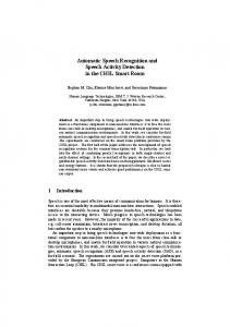
II. LAYERS IN AUTOMATIC SPEECH RECOGNITION A. Standard Approaches to Large-Vocabulary ASR As of this writing, state-of-the-art automatic speech recognition (ASR) systems incorporate quite a few layers of processing prior to the output of word sequences. The process starts with several layers of signal processing (e.g., windowing, short-term spectral analysis, critical band spectral integration and cepstral transformation). It is true that these stages are typically implemented with fixed parameters; on the other hand, there has been recent work that has shown improvements using learned parameters for a nonlinear function of the spectral values, inspired by the amplitude compression that is evident in human hearing [5]. However, even for other systems, it is quite common to transform the spectrum by compressing or expanding it in a process called vocal tract length normalization [6]. Despite its name, VTLN does not require any measure of the vocal tract, but uses statistical learning techniques to determine the maximum-likelihood compression/expansion of the spectrum for each clustered utterance or speaker (often derived from an unsupervised learning algorithm); these approaches are based on an underlying generative model. Another common component is Linear Discriminant Analysis (LDA) or its less constrained cousin, Heteroscedastic Linear Discriminant Analysis (HLDA), each of which is trained to maximize phonetic discrimination. This layer transforms cepstral features, typically over several past and future acoustic frames, into a new observation sequence for the recognition system. The resulting features are then used to train a large number of Gaussians that are used in combination to generate likelihoods for particular speech sounds in context. Note that both the individual Gaussians and their mixture coefficients are trained, and that Expectation–Maximization is used for training since the weighting of each component in the mixture is unknown a priori, even in training. Following training with a maximumlikelihood criterion, objective functions such as maximum mutual information (MMI) or minimum phone error (MPE) [7] are typically used to train the Gaussian parameters discriminatively. The parameters of this acoustic model are then altered further for testing by incorporating one of several related methods for adaptation, for instance Maximum-Likelihood Linear Regression (MLLR) [8]. The entire acoustic likelihood estimation subsystem is then used in combination with a language model probability estimation, which has been trained in a supervised fashion on a large number of words; additionally, there are usually multiple sources of word prediction information (such as large quantities of written text and smaller amounts of transcribed spoken words) so that weighting and backoff parameters must be learned. The interpolation coefficients between language and acoustic level log likelihoods are also learned, as are various other recognizer-specific parameters. Finally, the best recognizers typically incorporate multiple complete systems that combine their information at various levels, such as what is called cross-adaptation, in which training targets for one system comes from the other [9].

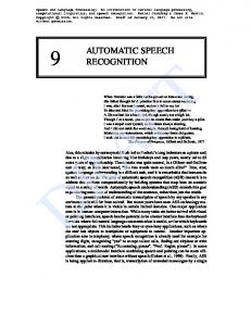
All of the above assumed a single stream of speech entering the system. However, it is becoming more common in practice to have at least two speech signal streams, one from each of two or more microphones. Combination techniques commonly incorporate unsupervised learning methods to determine the best combination of the microphone outputs [10]. This is far from a complete list of common ASR components; but it should suffice to show the reader that even ASR systems that do not routinely incorporate artificial neural networks or other explicitly layered machine learning mechanisms are both deep (many layers of computation) and wide (many different components combined). These layers often have fixed parameters, but in many cases they are learned, and often with an underlying generative model. The Section III will review a class of additional learned layers that have been added in some systems to nonlinearly process the features that are fed to the statistical engine. B. Tandem Approaches In 2000, as part of a European Telecommunications Standards Institute (ETSI) competition for a new Distributed Speech Recognition standard [11], an approach to speech recognition was developed that was called Tandem [12]. Drawing on MLP techniques developed in the context of computing discriminant emission probabilities for HMMs [13], this approach generated features for the HMM that were trained for phonetic discrimination. As in the earlier techniques, the MLP in the newer approach is trained with phone label targets, so that it estimates state or phone posterior probabilities; outputs from multiple MLPs are sometimes combined to improve the probability estimates. The typical initial system used a single nonlinear hidden layer. However, later architectures incorporated more layers; for instance the so-called TRAPS system used such an MLP for a half second of the time sequence of energies for each critical band of the spectrum (or for each set of three bands, with overlap) [14], followed by a combination component that comprised an additional MLP with its own hidden layer. This was learned separately, so that there was no attempt to back propagate errors all the way back through the system. A later form of this system called HATs [15] was trained by taking the input-to- hidden nonlinear transformations from each critical band and using their outputs to feed the final combination MLP (Fig. 2). In a number of large tasks (American English conversational telephone speech, American English broadcast news, Mandarin broadcast news, Arabic broadcast news), a further combination of HATs output and an MLP processed version of standard PLP features was used to provide significant (roughly 10% relative) reductions in errors. This was one of the largest reductions shown from any improvement in the systems under test [9]. C. Other Approaches At IBM, researchers developed a technique called Featurebased Minimum Phone Error (fMPE) [16], which incorporated the MPE error criterion at the feature level. In this approach,

MORGAN: DEEP AND WIDE: MULTIPLE LAYERS IN ASR

Fig. 1. Computational layers for standard single stream large vocabulary speech recognition acoustic model. Shaded boxes represent layers with at least some learned parameters. VTLN stands for Vocal Tract Length Normalization (defined in text). Not shown are the decision trees that determine the structure of the models in the statistical engine; these also have learned parameters.

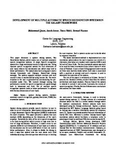
the features were generated by training a large number of Gaussians over the acoustic sequence2 and computing temporally local posteriors. In practice it provided similar improvements to either MPE training of the acoustic models or to the MLP-based approach described above. Combinations of these methods have also been explored in [17]. Other approaches have been built on a hierarchical feature approach, for instance training Tandem features for high temporal modulation frequencies and using them, appended to low temporal modulation frequencies as input for a second network generating Tandem features (Fig. 3). Thus, one path through the networks encountered four layers of processing by trained parameters while the other encountered two. This method provided significant improvement on a difficult ASR task requiring recognition of speech from meetings [18], and later was demonstrated to provide significant improvements in character error rate for a large-vocabulary Mandarin broadcast news evaluation [19]. D. Comments on Depth and Width For all of these approaches to improving speech recognition systems via modifications of the observation stream, it often was most natural to incorporate many layers of processing, and to 2The preliminary processing that comprises this sequence typically is either a set of mel frequency cepstral coefficients (MFCCs) or Perceptual Linear Prediction coefficients (PLP), each of which is computed over something like a 25-ms window and stepped forward every 10 ms.

9

Fig. 2. Computational layers for the TRAPS or HATS version of Tandem processing, where the first layer summarizes the front end processing from Fig. 1. All layers except the last have learned parameters. Each of the MLP layers has nonlinear hidden units. The critical band MLPs can either be trained separately from the combining MLP (as in HATs) or in one large training with connectivity constraints (as in Chen’s Tonotopic MLP). The simplified figure does not show that the input to the MLP stage is from the pre-smoothed spectral values, while the standard components of the feature vector are cepstral values with other transformations (e.g., derivatives, HLDA, etc.) All MLPs were trained with phone targets, and generated estimates of phone posteriors. Each output from the MLP is either taken prior to the final nonlinearity or else after computing the log probability. The linear transformation in this and later figures typically consists of principal component analysis (PCA), which requires unsupervised learning to determine the orthogonal dimensions with the greatest variance.

Fig. 3. Computational layers for hierarchical modulation processing [19]. The high temporal modulations (e.g., 10 Hz) are processed first, and the phone posteriors from the first MLP are used as input to the second along with low modulation frequency information, all coming from critical band energies over time (typically 5 seconds).

>

add them on (or insert them) into existing systems without re-engineering the entire structure. Instead, the standard capabilities of maximum likelihood or discriminative training methods were ultimately used to best accommodate the new transformations. In other words, at least for the difficult task of large vocabulary speech recognition, any successful system will be “deep,”

10

IEEE TRANSACTIONS ON AUDIO, SPEECH, AND LANGUAGE PROCESSING, VOL. 20, NO. 1, JANUARY 2012

in the sense of many layers of processing, and many of these layers will have parameters that are learned. Some layers will be trained using an underlying generative model, others will be trained in a purely discriminative manner, while in other cases both approaches will be used. However, the existence of multiple learned layers does not obviate the requirement for substantial width. In our experiments with conversational telephone speech, for instance, we found it useful to have MLP hidden layers with as many as 20 000 hidden sigmoidal units, resulting in over 8 million parameters for each of four different MLPs [20] (2 genders times 2 architectures, namely HATs and PLP-Tandem). While there are certainly speech processing tasks for which hidden layers can be much smaller, we have found that in practice, having sufficiently large widths can also be very important. In our work, we have typically found that using an insufficient number of units per layer can have a very large effect on the word error rate (although this saturates or can even slightly decline with too large a layer). Of course, it also clearly matters what any additional layer does. While in MLPs all of the computational layers tend to do the same thing, in larger systems such as the one shown in Fig. 1, the layers are often quite heterogeneous. Furthermore, systems often have a more complex topology than a straightforward layered structure—often there are parallel sidepaths, as in the hierarchical approach described in [19] and sketched in Fig. 3. In another hierarchical structure described in Pinto’s recent Ph.D. dissertation [21], the different layers of the hierarchy correspond to width of the acoustic context observed by each MLP; the first layer encompassing 90 ms of the cepstral input and the second layer taking as input 150–250 ms of the outputs from the first MLP. Section III describes some of the experiments over the last decade that demonstrated the value of both increasing width and depth in layered networks for large-vocabulary speech recognition. III. REVIEW OF SOME RELEVANT EXPERIMENTS In a 1999 ICASSP paper [4], we empirically demonstrated the utility of using a sufficiently large hidden layer for three-layer networks used in the hybrid HMM/MLP system [13]. The paper showed that for such a system there was an optimum range for the ratio between training patterns and number of parameters (between 10 and 40) when the maximum computation available was fixed. Without computational limits, given an early stopping learning approach (in which cross-validation on an independent set indicated when to stop training), the paper showed that increases in the number of parameters, as implemented through the increase of hidden layer size, provided large reductions in word error rate. This was an unsurprising result. However, it is still important to note that significantly increasing the width of the hidden layer was an effective way to derive the benefits one might expect from an increase in the number of learned parameters (see Table I below). In Barry Chen’s 2005 Ph.D. dissertation, he described a range of experiments with Tandem systems that use different topologies for their MLP transformations. In this experiment, as is typically the case for Tandem systems, the MLPs are trained on phonetic targets that are obtained

TABLE I WORD ERROR RATE PERCENTAGES WITH THE HYBRID HMM/ANN SYSTEM FOR BROADCAST NEWS SPEECH AND DIFFERING WIDTH MLPS (FROM [4])

Fig. 4. 15

2 51 MLP3.

Fig. 5. 15

2 51 MLP4.

via forced alignment on the training sentences using previously trained HMMs. The SRI system (DECIPHER) was used for both training and recognition [9]. Figs. 4–6 show the topologies for the systems of Table II. Note that while the bottom three rows, which incorporate an additional layer, show substantial improvements over the threelayer system, all three four-layer systems provide comparable improvements. This suggests that, at least for this task, which was large-vocabulary conversational telephone speech recognition, neither the precise topology nor the training approach (piece by piece or all at once) made any significant difference. More recently, we and others have explored the use of temporal and spectral filters as preprocessors of the time–frequency plane for multiple MLP streams that are used in Tandem style. This approach, shown in Fig. 7, is similar to the modulation filtering shown in Fig. 3, but in this case we did a broad range of spectro-temporal modulation filtering and channeled groups of these features into a number of MLP-transformed streams, leading to significant reductions in error, particularly for noisy test sets [22]. In our best result for noisy speech, we combined

MORGAN: DEEP AND WIDE: MULTIPLE LAYERS IN ASR

11

TABLE II

PLP+ REFERS TO HLDA-TRANSFORMED PLP AND ITS FIRST 3 TEMPORAL

DERIVATIVES, WHILE THE NEXT TWO ROWS GIVE RESULTS FOR A FEATURE STREAM AUGMENTED BY AN MLP NONLINEARLY TRANSFORMING 15 SPECTRAL ENERGIES OVER 51 FRAMES. MLP3 REFERS TO A THREE-LAYER MLP (ONE HIDDEN LAYER) AND MLP4 REFERS TO A FOUR-LAYER MLP (2 HIDDEN LAYERS). HAT AND MLP ARE BOTH 4-LAYER MLPS, BUT THE FORMER USES15 CRITICAL BAND MLPS TRAINED SEPARATELY WITH OUTPUTS USED TO FEED A 16TH COMBINING MLP, WHILE TMLP IS A SINGLE MLP WITH THE SAME CONNECTIONS THAT IS ALL TRAINED TOGETHER. THE NUMBER OF PARAMETERS IN THE MLP IS THE SAME. THE STAND-ALONE COLUMN REFERS TO USING A TANDEM FEATURE VECTOR ON ITS OWN, WHILE THE AUGMENTED COLUMN GIVES RESULTS FOR A FEATURE VECTOR COMPRISED OF THE PLP+ FEATURES AUGMENTED BY THE TANDEM FEATURES, WHICH IS THE WAY THAT OUR TANDEM FEATURES ARE GENERALLY USED. WER = WORD ERROR RATE FOR CONVERSATIONAL TELEPHONE SPEECH. FROM [15]

Fig. 6. Chen’s Tonotopic net (TMLP). When the top row of hidden layers are trained previously as part of individual three-layer MLPs, the diagram also represents Chen’s Hidden Activation TRAPs (or HATs).

Fig. 7. Spectro-temporal modulation filters implemented as streams of mel spectra over time and frequency with Gabor functions; for a four-stream case, each stream uses roughly 500 different filters providing output into an MLP. In this case the input layer for each MLP is wider than the hidden layer, as the latter uses only 160 units. An additional MLP is trained to generate weights for a linear combination of the phone posterior probability estimates coming out of the Gabor stream MLPs. For this MLP, the targets are derived from a determination of the best stream (closest phone classification to reference) on a development set. Details of this approach can be found in [22].

streams by weighting and summing each phone probability with its counterparts in the other streams, where the weights were generated as outputs from another MLP that had been trained using targets that were set to one for the best stream (according to frame classification with some moderate smoothing) and zero for the other streams. Thus we have found that not only width and depth are important, but also the choice of mechanism for weighting and/or selecting streams is important for handling diverse test sets whose properties may not match those available during training. IV. COMMENTARY AND SPECULATION For all of the methods described in the previous section, a key property was the computation of a number of different func-

tions in parallel, in addition to using multiple layers of computation. In some cases, particularly for noisy speech, the additional “width” (via hidden layer size or multiple streams of processing) provided dramatic improvements. The overall number of trained parameters was also a critical quantity, in some cases even more effective than adding additional layers, but probably the most important factor was the choice of transformations, which makes significant use of our experience with processing the speech signal. As noted in the introduction, the focus of this paper is on a class of largely heterogeneous layered systems, many of which provided greater width and less depth than the systems that are becoming known as Deep Belief Networks. The latter are just beginning to be tested for large-vocabulary speech recognition (at least with large amounts of training data relative to the number of trained parameters), and so this author has made no attempt to compare them to the methods described here. It is however worth noting that the two kinds of approaches are somewhat different. Deep Belief Networks,3 as for instance described in [2], incorporate layer-by-layer learning for a generative model in a homogeneous structure for tasks such as, e.g., phoneme recognition. In this approach, these stages of learning are typically followed by a globally discriminative training step incorporating error back propagation, which does not rely on a generative model. Consequently, one could either view the whole process as being a fundamentally generative architecture with some minor tuning at the end of the learning procedure, or else a fundamentally discriminative method with a clever form of initialization at the start. In the latter view, other types of initialization may serve equally well (for instance, a discriminatively trained set of weights for a previous, similar task). Such initializations (both using deep belief networks and weights from other tasks or data sets) are likely to be more important for examples with insufficient data, as one might find 3The common acronym for Deep Belief Networks is, understandably, DBN; this author has chosen to only use the expanded form given the acronym’s overlap with Dynamic Bayesian Networks, a previous method that still holds considerable interest in the speech community.

12

IEEE TRANSACTIONS ON AUDIO, SPEECH, AND LANGUAGE PROCESSING, VOL. 20, NO. 1, JANUARY 2012

with low resource languages (i.e., those for which there are currently insufficient amounts of manually labeled data to rely entirely on standard methods). Indeed, as noted by one of the pioneers of Deep Belief Networks [23], the ability to use many more parameters for a given amount of data (without overfitting) was one of the major design aims for deep learning networks. However, to the best of this author’s knowledge, there is currently insufficient experimental evidence to support comparative performance with and without deep learning initialization for large-vocabulary speech recognition tasks for which sufficient data is indeed available. After 60 years of speech recognition research, we find that error rates for difficult tasks are still unacceptably high. It is likely that using many layers of well-chosen computation, along with multiple streams of these layers, will be an important component of the solution. However, it is unlikely that a blind search using any clever machine learning technique will be sufficient to solve this problem. New approaches to learning over many layers may provide performance improvements on a number of tasks in speech and language processing. However, despite such advances, it could be the case that we will not make further substantial progress until we better understand what limitations in our signal representation and models are causing the errors. There have been a few steps in this direction. One was the Ph.D. dissertation of Chase [24], in which considerable effort was exerted towards the goal of showing the causes of individual errors. A more recent effort [25] provided a methodology for exploring the source of modeling errors, in particular showing which violations of the model assumptions were causing problems. The previously mentioned Pinto dissertation [21] also made use of Volterra series analysis to better understand the nature of the phonetic confusions arising from the particular structure. It could be the case that we will not be able to substantially improve speech recognition until we follow such approaches and learn what it is that we have to fix. In the meanwhile, we all continue to suggest clever ideas for improving the front end or the statistical engine, and these will provide some traction. Some of these may continue to be inspired by models of speech production or perception, given the relation of production mechanisms to the resulting signal, and the robustness of human speech recognition in comparison with its artificial counterpart. It should be noted that this paper only included topics pertaining to the acoustic model. The model for the sequence of words (the so-called language model), as well as any post processing of word sequence hypotheses that incorporates pragmatic knowledge about the application, are both extremely important. The processing of the outputs of the complete (acoustic and language model) statistical engine may be as important as any particular approach to machine learning for the models, or the processing of the feature inputs that has been the focus here. For further reading on previous milestones and possible directions for future progress in ASR, the reader is referred to [26] and [27] for a recent study by a number of us in the field. ACKNOWLEDGMENT The author would like to thank several colleagues for major contributions of the ideas that led to this paper: H. Bourlard

of IDIAP and EPFL, H. Hermansky of Johns Hopkins, and A. Stolcke of SRI. The author would also like to thank anonymous reviewers, (as well as O. Vinyals of ICSI and UCB, who provided internal criticism), who made important suggestions to improve the draft. Despite these contributions, the views expressed in this paper, and in particular the errors, can be blamed on the author alone. REFERENCES [1] K. H. Davis, R. Biddulph, and S. Balashek, “Automatic recognition of spoken digits,” J. Acoust. Soc. Amer., vol. 24, no. 6, pp. 627–642, 1952. [2] G. Dahl, M. Ranzato, A. Mohamed, and G. E. Hinton, “Phone recognition with the mean-covariance restricted Boltzmann machine,” in Advances in Neural Information Processing 23. Cambridge, MA: MIT Press, 2010. [3] S. S. Viglione, “Applications of pattern recognition technology,” in Adaptive Learning and Pattern Recognition, J. M. Mendel and K. S. Fu, Eds. New York: Academic, 1970, pp. 115–161. [4] D. Ellis and N. Morgan, “Size matters: An empirical study of neural network training for large vocabulary continuous speech recognition,” in Proc. ICASPP, 1999, pp. 1013–1016. [5] Y.-H. Chiu, B. Raj, and R. Stern, “Learning based auditory encoding for robust speech recognition,” in Proc. ICASSP, 2010, pp. 428–4281. [6] J. Cohen, T. Kamm, and A. Andreou, “Vocal tract normalization in speech recognition: compensation for system systematic speaker variability,” J. Acoust. Soc. Amer., vol. 97, no. 5, pt. 2, pp. 3246–3247, 1995. [7] D. Povey, “Discriminative training for large vocabulary speech recognition,” Ph.D. dissertation, Cambridge Univ., Cambridge, U.K., 2004. [8] C. J. Leggetter and P. C. Woodland, “Maximum likelihood linear regression for speaker adaptation of continuous density HMMs,” Speech Commun., vol. 9, pp. 171–186, 1995. [9] A. Stolcke, B. Chen, H. Franco, V. R. R. Gadde, M. Graciarena, M.-Y. Hwang, K. Kirchhoff, A. Mandal, N. Morgan, X. Lei, T. Ng, M. Ostendorf, K. Sonmez, A. Venkataraman, D. Vergyri, W. Wang, J. Zheng, and Q. Zhu, “Recent innovations in speech-to-Text transcription at SRIICSI-UW,” IEEE Trans. Audio, Speech, Lang. Process., vol. 14, no. 5, pp. 1729–1744, Sep. 2006. [10] M. Seltzer, B. Raj, and R. Stern, “Likelihood maximizing beamforming for robust hands-free speech recognition,” IEEE Trans. Speech Audio Process., vol. 12, no. 5, pp. 489–498, Sep. 2004. [11] H.-G. Hirsch and D. Pearce, “The aurora experimental framework for the performance evaluation of speech recognition systems under noisy conditions,” in Proc. ISCA ITRW ASR2000 Autom. Speech Recognition: Challenges for the Next Millennium, Paris, France, Sep. 2000. [12] H. Hermansky, D. Ellis, and S. Sharma, “Tandem connectionist feature extraction for conventional HMM systems,” in Proc. ICASSP, Istanbul, Turkey, Jun. 2000, pp. 1635–1638. [13] H. Bourlard and N. Morgan, Connectionist Speech Recognition: A Hybrid Approach. Norwell, MA: Kluwer, 1993. [14] H. Hermansky and S. Sharma, “TRAPS—Classifiers of temporal patterns,” in Proc. 5th Int. Conf. Spoken Lang. Process. (ICSLP’98), 1998, pp. 1003–1006. [15] B. Y. Chen, “Learning discriminant narrow-band temporal patters for automatic recognition of conversational telephone speech,” Ph.D. dissertation, Univ. of California, Berkeley, 2005. [16] D. Povey, B. Kingsbury, L. Mangu, G. Saon, H. Soltau, and G. Zweig, “fPME: Discriminatively trained features for speech recognition,” in Proc. IEEE ICASSP’05, 2005, pp. 961–964. [17] J. Zheng, O. Cetin, M.-Y. Hwang, X. Lei, A. Stolcke, and N. Morgan, “Combining discriminative feature, transform, and model training for large vocabulary speech recognition,” in Proc. IEEE ICASSP’07, Honolulu, HI, Apr. 2007, pp. 633–636. [18] H. Hermansky and F. Valente, “Hierarchical and parallel processing of modulation spectrum for ASR applications,” in Proc. IEEE ICASSP’08, 2008, pp. 4165–4168. [19] F. Valente, M. Magamai-Doss, C. Plahl, and S. Ravuri, “Hierarchical processing of the modulation spectrum for GALE Mandarin LVCSR system,” in Proc. Interspeech’09, Brighton, U.K., 2009. [20] N. Morgan, Q. Zhu, A. Stolcke, K. Sonmez, S. Sivadas, T. Shinozaki, M. Ostendorf, P. Jain, H. Hermansky, D. Ellis, G. Doddington, B. Chen, O. Cetin, H. Bourlard, and M. Athineos, “Pushing the envelope—Aside,” IEEE Signal Process. Mag., vol. 22, no. 5, pp. 81–88, Sep. 2005.

MORGAN: DEEP AND WIDE: MULTIPLE LAYERS IN ASR

[21] J. P. Pinto, “Multilayer perceptron based hierarchical acoustic modeling for automatic speech recognition,” Ph.D. dissertation, EPFL, Lausanne, Switzerland, 2010. [22] S. Zhao, S. Ravuri, and N. Morgan, “Multi-stream to many-stream: Using spectro-temporal features for ASR,” in Proc. Interspeech, Brighton, UK, 2009, pp. 2951–2954. [23] G. Hinton, personal communication. 2010. [24] L. Chase, “Error-responsive feedback mechanisms for speech recognizers,” Ph.D. dissertation, Robotics Inst., Carnegie Mellon Univ., Pittsburgh, PA, 1997. [25] S. Wegmann and L. Gillick, Why has (reasonably accurate) automatic speech recognition been so hard to achieve? Nuance Commun., 2009 [Online]. Available: http://web.mit.edu/kenzie/www/wegmann/wegmann_gillick_why.pdf [26] J. M. Baker, L. Deng, J. Glass, S. Khudanpur, C. Lee, N. Morgan, and D. O’Shaughnessy, “Research developments and directions in speech recognition and understanding, part 1,” IEEE Signal Process. Mag., vol. 26, no. 3, pp. 75–80, May 2009. [27] J. M. Baker, L. Deng, J. Glass, S. Khudanpur, C. Lee, N. Morgan, and D. O’Shaughnessy, “Research developments and directions in speech recognition and understanding, part 2,” IEEE Signal Process. Mag., vol. 26, no. 4, pp. 78–85, Jul. 2009.

13

Nelson Morgan (S’76–M’80–SM’87–F’99) received the Ph.D. degree in electrical engineering from the University of California, Berkeley, in 1980. He is the Director of the International Computer Science Institute, Berkeley, CA, where he has worked on speech processing since 1988. He is Professor-inResidence in the Electrical Engineering Department of the University of California, Berkeley. In previous incarnations, he worked on EEG signal processing at the EEG Systems Laboratory and on speech analysis and synthesis at National Semiconductor. He has over 200 publications including three books, the most recent of which is a text on speech and audio processing coauthored with signal processing pioneer B. Gold (a new revision of which is now being prepared with coauthor D. Ellis of the University of Columbia). His current interests include the incorporation of insights from studies of auditory cortex to practical speech recognition algorithms. Prof. Morgan is a former and returning member of the IEEE Signal Processing Society Spoken Language Technical Committee, a former editor-in-chief of Speech Communication (and currently on its editorial board), and is now on the editorial board of IEEE SIGNAL PROCESSING MAGAZINE. He is a member of the International Speech Communication Association, and is on its Advisory Council. In 1997 he received the Signal Processing Magazine best paper award (jointly with H. Bourlard).