The rendering is done on a GPU via OpenGL API. ..... Graph., 13(2), pp. 261-. 271, (2007). .... [33] R.C. Veltkamp, F.B. ter Harr, SHREC 2007 3D Shape. Retrieval ...
Takahiko Furuya, Ryutarou Ohbuchi, Dense Sampling and Fast Encoding for 3D Model Retrieval Using Bag-of-Visual Features, accepted, ACM International Conference on Image and Video Retrieval, July 8-10, 2009, Santorini, Greece.
Dense Sampling and Fast Encoding for 3D Model Retrieval Using Bag-of-Visual Features Takahiko Furuya
Ryutarou Ohbuchi
University of Yamanashi 4-3-11 Takeda, Kofu-shi Yamanashi-ken, 400-8511, Japan +81-55-220-8570
University of Yamanashi 4-3-11 Takeda, Kofu-shi Yamanashi-ken, 400-8511, Japan +81-55-220-8570
snc49925AT gmail.com
ohbuchiAT yamanashi.ac.jp
ABSTRACT
1. INTRODUCTION
Our previous shape-based 3D model retrieval algorithm compares 3D shapes by using thousands of local visual features per model. A 3D model is rendered into a set of depth images, and from each image, local visual features are extracted by using the Scale Invariant Feature Transform (SIFT) algorithm by Lowe. To efficiently compare among large sets of local features, the algorithm employs bag-of-features approach to integrate the local features into a feature vector per model. The algorithm outperformed other methods for a dataset containing highly articulated yet geometrically simple 3D models. For a dataset containing diverse and detailed models, the method did only as well as other methods. This paper proposes an improved algorithm that performs equal or better than our previous method for both articulated and rigid but geometrically detailed models. The proposed algorithm extracts much larger number of local visual features by sampling each depth image densely and randomly. To contain computational cost, the method utilizes GPU for SIFT feature extraction and an efficient randomized decision tree for encoding SIFT features into visual words. Empirical evaluation showed that the proposed method is very fast, yet significantly outperforms our previous method for rigid and geometrically detailed models. For the simple yet articulated models, the performance was virtually unchanged.
We have previously proposed a shape-based 3D model retrieval algorithm that aimed at handling both articulated and rigid models [24]. The algorithm is appearance based, so it accepts a diverse set of 3D shape representations so far as it can be rendered as range images. To achieve invariance to articulation and/or global deformation, the algorithm employs a set of multi-scale, local, visual features to describe a 3D model. After normalizing the model for its position and scale, a set of depth images of the model is generated by using multiple virtual cameras looking inward at the model. From each depth image, dozens of local visual features are extracted. We used a saliency-based local image feature Scale Invariant Feature Transform (SIFT) by David Lowe [19]. The SIFT first detects, in a multi-scale image pyramid, salient points at which human visual system would presumably attracted to. The SIFT then extracts, at each salient point, a feature that encodes position, orientation, and scale of gray-scale gradient change. Typically, a 3D model is rendered into 42 depth images, each one of which then produces 30 to 50 salient points. Thus, a 3D model is described by a set of 1.5k SIFT features. Directly comparing a pair of such feature sets would be too expensive, especially to search through a 3D model database containing a large number of models. To reduce the cost of model-to-model similarity comparison, the set of thousands of visual features is integrated into a feature vector per model by using bag-of-features (BoF) approach (e.g., [6, 20, 29, 35]). The BoF approach vector quantizes, or encodes, the SIFT feature into a representative vector, or “visual word”, using a previously learned codebook. The visual words are accumulated into a histogram, which becomes the feature vector.
Categories and Subject Descriptors H.3.3 [Information Search and Retrieval]: Information filtering. I.3.5 [Computational Geometry and Object Modeling]: Surface based 3D shape models. I.4.8 [Scene Analysis]: Object recognition.
General Terms Algorithms, Experimentation.
Keywords Content-based retrieval, multi-scale feature, bag-of-features, Scale Invariant Feature Transform, GPU based algorithms, randomized decision tree, approximate nearest neighbor, hashing.
Permission to make digital or hard copies of all or part of this work for personal or classroom use is granted without fee provided that copies are not made or distributed for profit or commercial advantage and that copies bear this notice and the full citation on the first page. To copy otherwise, to republish, to post on servers or to redistribute to lists, requires prior specific permission and/or a fee. CIVR '09, July 8-10, 2009 Santorini, GR Copyright © 2009 ACM 978-1-60558-480-5/09/07... $5.00
Experimental evaluation of our previous algorithm showed that it works quite well for the McGill Shape Benchmark (MSB) [37] which contains highly articulated but geometrically simple shapes. For the MSB, the method significantly outperformed all previous methods we have compared against, including the Light Field Descriptor (LFD) [5] and the Spherical Harmonics Descriptor (SHD) [17]. However, for the Princeton Shape Benchmark (PSB) [26], which contains diverse shapes having more geometric details but with virtually no articulation, the method performed as well but not better than the peers. Also, our previous algorithm has a high computational cost. Rendering tens of depth images, extracting thousands of local visual features per model, and vector-quantizing these features can be expensive. In this paper, we propose a faster and more accurate 3D model retrieval algorithm using local visual features. The proposed algorithm aims at high retrieval performance for both rigid and detailed models of the PSB and simple yet articulated models of
Takahiko Furuya, Ryutarou Ohbuchi, Dense Sampling and Fast Encoding for 3D Model Retrieval Using Bag-of-Visual Features, accepted, ACM International Conference on Image and Video Retrieval, July 8-10, 2009, Santorini, Greece. the MSB. To do so, our proposed algorithm extracts SIFT features at hundreds of densely and randomly placed points per depth image, as opposed to dozens of salient points detected by the original SIFT. This dense sampling increases the number of local features per model from 1.5k to 13k with according increase the computational cost, especially at SIFT feature extraction and vector quantization steps. To reduce computation time, our proposed algorithm utilizes a very fast vector quantization algorithm based on Extremely Randomized Clustering Trees (ERC Trees) [9]. The algorithm also employs a Graphics Processing Unit (GPU) based implementation of the SIFT algorithm SiftGPU by Wu [36] to quickly extract SIFT features. Our empirical evaluation showed that the proposed algorithm is more accurate and faster than our previous algorithm [24]. Retrieval performance measured in R-precision [3] of the PSB (test set) has jumped from 45.1% of the previous method [24] to 55.8% of the proposed method. For the other two databases we experimented with, the MSB and the Engineering Shape Benchmark (ESB) of machine parts models [15], retrieval performances of the new method tied with our previous method. The remaining parts of this paper have the following structure. After reviewing previous work, we will describe the proposed algorithm in Section 3. Empirical evaluation of the proposed algorithm will be described in Section 4. Section 5 will present the summary and future work.
2. RELATED WORK Recent interest in content-based retrieval of 3D models has produced a quickly expanding body of work on the subject [12, 30, 33]. Most 3D model retrieval method would require invariance against geometrical transformation of at least up to similarity transformation. Only a small minority, however, addressed the issue of invariance to articulation or global deformation. To achieve articulation invariance, a class of methods employed topological matching approaches [4, 10, 28, 31]. This class of methods, however, is difficult to implement and prone to presence of geometrical and/or topological error and/or noise. Another class of methods, e.g., [7, 8, 13, 14] uses curvature and other local geometrical and/or topological properties of manifold surfaces as local or global feature for pose invariant shape comparison. Of these, the method by Jain et al [13, 14] explicitly addresses articulation invariance. It employs a joint geometrical-topological analysis based on mesh spectral analysis. This class of methods, however, assumes manifold meshes so they can’t be applied to a large subclass of 3D models. Yet another class of approaches uses a set of local features for articulation invariant 3D model comparison [2, 16, 18, 24, 27]. This class of methods typically samples the surface of the model by using either 2D [2, 11, 16, 18, 24] or 3D [27] local features. One of the issues with the localfeature based approach is the cost of comparing and storing a set of large number of features per model. Assuming n features per model, comparing all the pairs of features of a pair of models would cost O(n2 ) . For a database of nontrivial size, such method would take too long for a search. Cost of storage is also significant. For example, a SIFT feature used in [24] is a 128dimensional vector. Assuming 1k SIFT features per model and 4Byte float representation of an element, a set of SIFT features per model would require 512kByte for its storage. To solve this issue of computational and storage cost, our previous method [24] adopted a bag-of-features (BoF) approach. In the field of object recognition from 2D images, BoF is one of
the most popular and powerful approaches to compare sets (often having unequal sizes) of features [6, 20, 29, 35]. The approach encodes a given local feature into one of several hundreds to thousands of visual word, by using a visual codebook. The visual codebook is often generated by performing k-means clustering on the training set of local features by setting k to the size of vocabulary Nv Then, for each 3D model, a histogram of visual words is created, whose number of bins equals to the size of vocabulary. The histogram is the feature vector for the 3D model. Note here that locations of local features in each image are ignored. Experiments showed that, for a set of geometrically less detailed yet highly articulated models of the MSB [37], our previous method performed significantly better than the other methods we have compared against. However, for a set of models found in the PSB, which are more diverse in shape and contains more details but has much less articulation than the MSB, the method is only as good as those previous methods. Our observation was that the salient point detector of the SIFT algorithm has been “falsely” triggered by details of some of more complex 3D models, while ignoring important yet monotone region of the images. For example, in Figure 2(d), which is generated by our previous algorithm [24], the depth image of the potted plant produced a large number of small scale features near the leaves. These features, being scale invariant, could match local geometrical feature of other models that are similar in shape yet completely different in scale. The potted plant, consequently, could potentially match shapes having completely different overall shape. On the other hand, an important large scale feature,
Render range images
Number of views Ni View 1 View 2
View Ni …
Extract SIFT features
Encode features Generate histogram
Bag-offeatures Nv clusters
Bags-ofvisual words
Vocabulary size Nv Histogram Feature vector
(5
8 4)
(7
5 4)
Compute distance Distance Figure 1. Local visual features are integrated into a feature vector by using bag-of-feature approach for an efficient model-to-model similarity (or distance) computation.
Takahiko Furuya, Ryutarou Ohbuchi, Dense Sampling and Fast Encoding for 3D Model Retrieval Using Bag-of-Visual Features, accepted, ACM International Conference on Image and Video Retrieval, July 8-10, 2009, Santorini, Greece. 2.
3.
(a) BF-SSIFT, Np=47
(b) BF-DSIFT, Np=327
(c) BF-GSIFT, Np=336 4.
(d) BF-SSIFT, Np=383
(e) BF-DSIFT, Np=342
(f) BF-GSIFT, Np=336
Figure 2. Example of feature points using BF-SSIFT (a)(d), BF-DSIFT (b)(e), and BF-GSIFT (c)(f). in this case a large trapezoidal shape of the pot, is underrepresented in the bag of features. For simpler shapes having less details, e.g. that of MSB, original SIFT with salient point detector worked very well. However, for the PSB, which contains models having considerably more detail, the salient points are not balanced representation of the features of the model. This observation led us to the proposed algorithm that samples each depth image of a 3D model more uniformly and densely. Such sampling would produce “balanced” representation of local geometrical features in the bag of features, and consequently, in the histogram of visual words that describes the 3D model. We choose dense and random sampling of the image, so the proposed method is called Bag-of-Features Dense SIFT (BF-DSIFT) algorithm. To differentiate, our original algorithm having the salient point detector is called Bag-of-Features Salient SIFT (BFSSIFT) algorithm. The increase in the number of features due to dense sampling, however, ups the cost of SIFT feature extraction and feature encoding. For example, a typical number of features per 3D model and a typical size of vocabulary for the BF-SSIFT are both 1.5k. For the BF-DSIFT, the number of features and vocabulary size increases to 11k and 10k~20k, respectively. To overcome such an increase in the number of local features, our proposed algorithm employs a GPU-based SIFT feature extractor and a very fast tree-based encoder for a significant speedup.
3. ALGORITHM We first review our previous algorithm, the BF-SSIFT, in the next section. Improvements made for the BF-DSIFT algorithm, that are, the dense visual feature sampling and fast feature encoding, will be described in Section 3.2 and Section 3.3, respectively.
3.1 Review of the BF-SSIFT algorithm The BF-SSIFT algorithm compares 3D models by following the steps below, which are illustrated in Figure 1. 1.
Pose normalization with respect to position and scale: The BF-SSIFT performs pose normalization only for position and scale so that the model is rendered at an appropriate position with an appropriate size in each of the multiple-view images. Pose normalization is not performed for rotation.
5. 6.
Multi-view rendering: Render range images of the model from N i viewpoints placed uniformly and regularly on the view sphere surrounding the model. The rendering is done on a GPU via OpenGL API. SIFT feature extraction: From the range images, extract local, multi-scale, multi-orientation, visual features by using Vedaldi’s implementation SIFT++ [32] of thethe SIFT [19] algorithm. The original SIFT algorithm first detects salient points, and then computes 128D SIFT feature at each of the salient points. Feature encoding: Encode a local feature into a visual word from a vocabulary of size N v by using a visual codebook. Prior to the retrieval, the visual codebook is learned, unsupervised, from tens of thousands of features extracted from a set of models, e.g., the models in the database to be retrieved. The encoding, or vector quantization, step is a nearest point query in a high dimensional (128D) feature space. It is implemented as a linear search through a set of Nv representative vectors. Histogram generation: Encoded local features or “visual words” are accumulated into a histogram having N v bins, which then becomes the feature vector of the 3D model. Distance computation: Dissimilarity among a pair of feature vectors (the histograms) is computed by using Kullback-Leibler Divergence (KLD); n
D ( x, y ) =
∑ ( y − x ) ln x i
i =1
i
yi
(1)
i
where x = ( xi ) and y = ( yi ) are the feature vectors and n is the dimension of the vectors. The KLD is sometimes referred to as information divergence or relative entropy.
3.2 Dense Sampling In the proposed BF-DSIFT, we employed dense random sampling of a range image by SIFT features. We wanted to concentrate samples on or near the 3D object, not on the background, of the range image. To do so, for each image in the multi-scale image pyramid of the SIFT algorithm [19], Np pixels to be sampled are drawn randomly from pixels having non-zero intensity value. A range image is rendered with zero pixel value as its background, and images in the SIFT pyramid are blurred according to their scale in the pyramid. Thus, a pixel from an images in the SIFT pyramid that has non-zero value is located on or near, but not far from, the image of the 3D model. As non-zero pixels are different for each image in the SIFT image pyramid, the positions of samples are different across scales in the SIFT pyramid. For comparison, we implemented another dense sampling strategy, which samples the image at regular grid points. We call the method Bug-of-Features Grid SIFT (BF-GSIFT). In the BFGSIFT, positions of the SIFT samples may overlap across scale in the SIFT image pyramid, as the image down-sampling for constructing the pyramid is performed by halving image after low-pass filtering. If we set the number of samples per depth image Np, and the number of views Ni, the total number of samples per 3D model N f = N p ⋅ N i . Typically, we use Ni=42 and Np~300 so we have Nf~12k. To accelerate extraction of a large number of SIFT features, we adopted the SiftGPU by Wu [36], which is a GPU implementation of the Vedaldi’s SIFT++ [32]. Given a gray-scale image, the SiftGPU does all the work of the SIFT on a GPU; construction of a multiresolution image pyramid, detection of
Takahiko Furuya, Ryutarou Ohbuchi, Dense Sampling and Fast Encoding for 3D Model Retrieval Using Bag-of-Visual Features, accepted, ACM International Conference on Image and Video Retrieval, July 8-10, 2009, Santorini, Greece. salient points, and extraction of SIFT features at the salient points. Our preliminary experiment using BF-SSIFT showed that the difference in retrieval performance between SIFT++ on a CPU and SiftGPU on a GPU is negligible [25]. For the dense sampling of BF-DSIFT, we modified the SiftGPU to disable salient point detector and to add the capability to accept from the CPU a list of pixels at which SIFT features are exracted. As a detail, our modified version of the SiftGPU doesn’t perform image upsampling in creating multi-resolution image pyramid. Our previous experiments showed no difference in retrieval performance with or without the up-sampling. Figure 2 shows, for two depth images, examples of sample points generated by using the BF-SSIFT (Figure 2(a), 2(d)), the BFDSIFT (Figure 2 (b), 2(e)), and the BF-GSIFT (Figure 2(c), 2(f)). The BF-DSIFT placed roughly the same number of samples on depth images of both human and potted plant models. The BFSSIFT, on the other hand, placed many more points on the image of potted plant model than the human model. Note also that the BF-DSIFT placed more samples on featureless parts, e.g., on or near the pot and the torso. The BF-GSIFT sampled regularly and uniformly regardless of the image features across image scales.
3.3 Fast Encoding Encoding of a local visual feature consists of two-steps; 1. 2.
Codebook learning: Prior to retrieval, find representative vectors in the feature space given a set of feature vectors for training. This amounts to clustering of feature points. Encoding (or vector quantization): Given a new vector, find the representative vector closest to the new vector. This is a nearest neighbor query in a high dimensional space.
In our original algorithm [24], we performed the codebook generation by using k-means clustering. For 50k training samples each having 128D and a vocabulary size of 1k, the k-means algorithm took about 200s to complete. While slow, especially when the vocabulary size Nv and the number of training samples Nt are large, the cost was acceptable since it needs to run only once as a preprocessing step. The k-means algorithm has spatial complexity of O ( d ⋅ Nt ) and temporal complexity of O ( d ⋅ Nt ⋅ Nv ) , given the dimension of the feature d, the number of training samples Nt, and the number of vocabularies Nv. For the vector quantization step, our previous algorithm [24] used a brute-force linear search approach that requires O ( N v ⋅ N f ) comparison per 3D model. This was barely acceptable for the SSIFT that produces Nf~1.5k features per model. However, for a set of SIFT features sampled densely would have Nf~11k, we needed a more efficient coder, or vector quantizer. To this end, we compared three algorithms for nearest neighbor search, the Extremely Randomized Clustering Trees (ERC-trees) algorithm by Guerts, et al [9], the locality sensitive hashing (LSH) algorithm by Andoni [1] in a library called E2LSH, and a kd-tree based approximate nearest neighbor (ANN) algorithm by Mount et al [21]. We implemented the ERC-tree ourselves. For the other two methods, we used the libraries cited. The ERC-trees algorithm is a combination of codebook learning and vector quantization algorithms so a separate clustering algorithm is not required. As the name suggests, the ERC-tree is a randomized tree-based clustering algorithm which subdivides the feature space into a half by each added tree node. Each subdivision is done by a hyper plane perpendicular to one of the coordinate axes. For each subdivision, the algorithm first
randomly picks the dimension (or axis) to subdivide, and then randomly chooses the point (a scalar value) on the axis at which a separating hyperplane is placed. Subdivision of the feature space continues until the number of data points per subspace is below a set parameter Smin. While the Smin affects the number of vocabulary Nv, the actual value of Nv differ for each trial due to the randomized nature of the algorithm. The Nv can also be controlled by pruning the tree, but we don’t perform any pruning. Moosemann et al in [20] suggested that the fully grown tree without pruning performed better for visual object recognition. Since the feature space is subdivided into subspaces by a set of axis aligned hyper planes, the quality of the resulting cluster may not be as good as those produced by other methods, e.g., k-means. However, the ERC tree is very fast for both training (clustering) and for coding. In the following, we add postfix “-E” or “-k” after the method name (e.g., BF-SSIFT) to indicate the clustering algorithm used. The letter “E” indicates the use of ERC-tree for clustering and vector quantization, while the letter “k” indicates the use of k-means for clustering combined with linear search. The kd-tree is a well-known spatial data structure often used for proximity queries. An approximate nearest neighbor search library for a high dimensional data by Mount et al [21] is based on kdtree. It subdivides the feature space by axis-aligned hyperplanes until the resulting subspace is smaller than the hypersphere of radius ε. To vector quantize a feature vector, the tree is traversed down to leaf to find the smallest subspace enclosing the feature. Then, n feature points contained in the hypersphere near the query point is searched for the closest representative vector. The locality sensitive hashing in the E2LSH library [1] employs a set of L hash functions that maps d dimensional feature vector onto K dimensional vector. The hash functions are chosen so that features close in the original d-dimensional feature space collide in the K-dimensional space produce by the hash function. To vector quantize a feature, the feature is hashed into a bucket, and the overflow list of the bucked is searched linearly for the nearest representative vector. While the K and L are parameters, the E2LSH has the ability to choose optimal set of K and L values given a training set of features. As both the ANN and the E2LSH are nearest neighbor search algorithm without codebook learning, we combine these two nearest neighbor search algorithms with the k-means clustering for codebook learning. Table 1 summarizes the spatial and temporal complexity of the algorithms. Actual running time of course would be determined various constants and real-world parameters. Table 1. Computational complexities of the nearest neighbor search algorithms compared. Spatial complexity
Temporal complexity
Linear search
O ( Nv )
O ( Nv )
ERC-tree
O ( Nv )
O ( log Nv )
kd-tree
O ( Nv )
O ( n + log Nv )
E2LSH
O ( Nv ⋅ L )
O ( n + L)
4. EXPERIMENTS AND RESULTS We experimentally evaluated the following; (1) Codebook learning and encoding algorithms. (2) Sampling strategy, number of features, and retrieval performance. (3) Vocabulary size and retrieval performance.
Takahiko Furuya, Ryutarou Ohbuchi, Dense Sampling and Fast Encoding for 3D Model Retrieval Using Bag-of-Visual Features, accepted, ACM International Conference on Image and Video Retrieval, July 8-10, 2009, Santorini, Greece. (4) Performance comparison with other methods. We performed the experiments using three benchmark databases: the MSB [37] for highly articulated but less detailed shapes, the PSB [26] for a set of diverse and detailed shapes, and the ESB [15] for mechanical parts. The MSB consists of 255 models in 10 classes. The MSB include such articulated shapes as “humans”, “octopuses”, “snakes”, “pliers”, and “spiders”. The PSB contains two equal-sized subsets, the training set and test set, each consisting of 907 models and about 90 classes. For our evaluation, we used the PSB test set partitioned into 92 classes. The PSB contains a more diverse set of 3D shapes than the MSB. The ESB contains 867 models divided into 45 classes and has 45 out-ofsample query models. The same database is used for codebook training and retrieval experiments. That is, the codebook generated by using the MSB, for example, is used to query the MSB. We used the training set size N t = 50,000 of SIFT features extracted from multi-view images of models in a database. Both for training and for query experiments, range images size of 256 × 256 pixels is used. As the performance index, we used R-precision [3]. R-precision is a ratio, in percentile, of the models retrieved from the desired class C k (i.e., the same class as the query) in the top R retrievals, in which R is the size of the class Ck . Note that, in this paper, we treat the query model found in the retrieval result as one of correct retrievals. As such, the R-precision figure is higher than some of the other publications if the query model is drawn from the database to be queried.
4.1 Codebook Learning and Encoding Algorithms We first compared, using BF-DSIFT and PSB test set, the cost codebook learning and encoding between the k-means and the ERC-tree algorithms. To train, we used the PSB test set, the number of view orientations Ni=42, and the number of training samples Nt=50k. Training samples are randomly subsampled from the set of SIFT features generated from the PSB test set. We fixed the number of features per image at Np=300, so the number of features per model Np~12k. Table 2 shows that the ERC-tree is much faster than the k-means clustering and that the increases in cost due to vocabulary size Nv is much less marked for the ERC-tree than k-means. Table 3 shows that the k-means has slightly better retrieval performance (~1.5%) than the ERC-tree. Also, for both ERC-tree and k-means, retrieval performance improves with Nv. The codebook due to ERC-tree has slightly less discriminative power since the clusters it produces have axis-aligned hyper planes as their boundaries. Table 4 shows the breakdown of computation time for the BFDISFT algorithm measured by using the PSB and Ni=42. It compares four encoders, that are, the brute force (linear search) method indicated by “br”, the kd-tree based method indicated by “kd”, the locality sensitive hashing indicated by “lsh”, and the ERC-tree indicated by “erc” in the “R/S/V/D” column. All the BF-DSIFT results uses GPU for rendering, GPU for SIFT feature extraction, and table lookup to evaluate log() function used in the Kullback-Leibler divergence. (See table legends.) The table also shows the timings for the BF-SSIFT algorithm, both the original version (C/C/br/F) [24] and the accelerated version by using GPU and table lookup (G/G/br/T) [25]. Please note that the number of features Nf for the BF-SSIFT is 1.3k/model, while that of the BF-
DSIFT is 13k/model. Also, the BF-SSIFT used vocabulary size Nv=1,000, while the BF-DSIFT used vocabulary size Nv=10,000. Table 4 is a bit cluttered, but several observations can be made. First, the BF-DSIFT using kd-tree and ERC-tree for the vector quantizer are much faster than the others while achieving retrieval performance 10% better in R-precision (RP) than the original BFSSIFT. This performance gains shows the effectiveness of the random, dense sampling. Please note that the BF-DSIFT took less time than the BF-SSIFT despite the fact that both number of features per model Nf and the vocabulary size Nv is nearly ten times more in the BF-DSIFT than in the BF-SSIFT. The reduction in execution time is brought about by the combination of GPUbased feature extraction and ERC-tree encoder. If we compare the four encoders for their speed, the linear search used in our original algorithm is obviously the slowest. The kdtree and the ERC-tree are about equal both in terms of speed and retrieval performance. The LSH algorithm is 4 times slower than the other two, and is a bit lower in performance. If we count in the one-time cost of codebook learning, the ERC-tree has an advantage over the others as the kd-tree requires expensive kmeans clustering for codebook learning. Table 2. Time in seconds to train codebook using the kmeans and the ERC-tree algorithms.
k-means clustering ERC-Tree clustering
Number of vocabulary Nv 1,000 5,000 10,000 230.36 1289.29 2871.16 5.83 6.66 7.88
Table 3. Retrieval performance in R-precision [%].
k-means+Linear seaerch ERC-Tree encoder
Number of vocabulary Nv 1,000 5,000 10,000 51.72 55.64 56.68 51.77 54.07 55.30
Table 4. Computational cost break down for the DSIFT algorithms using various encoders. Implementation Computation time [s] R/S/V/D Render SIFT VQ Dist. Total SSIFT C/C/br/F 3.28 8.61 14.53 0.1043 26.5 SSIFT G/G/br/T 0.16 0.74 14.53 0.0056 15.4 DSIFT G/G/br/T 0.16 1.73 222.96 0.0361 224.9 DSIFT G/G/kd/T 0.16 1.73 0.74 0.0361 2.7 DSIFT G/G/lsh/T 0.16 1.73 8.47 0.0361 10.4 DSIFT G/G/erc/T 0.16 1.73 0.56 0.0361 2.5 Table legends on “Implementation R/S/V/D” R : Rendering S : SIFT V : VQ C: SIFT++ on br: brute force C: CPU CPU kd: kd-tree G: GPU G: SiftGPU on lsh: LSH GPU erc: ERC-Tree
RP [%] 45.52 45.70 56.68 55.54 53.65 55.30
D : Distance F: log function evaluation T: table lookup
4.2 Sampling strategy, number of features, and retrieval performance In this experiment, we try to find relationship between the number of features and retrieval performance. We also compare two dense sampling strategies, BF-DSIFT and BF-GSIFT. Number of features Nf can be controlled by (1) the number of view Ni, (2) the
Takahiko Furuya, Ryutarou Ohbuchi, Dense Sampling and Fast Encoding for 3D Model Retrieval Using Bag-of-Visual Features, accepted, ACM International Conference on Image and Video Retrieval, July 8-10, 2009, Santorini, Greece. number of sample points per depth image Np, or both. We compared the following four cases using the PSB dataset. In the experiment, we used the values Ni∈{6, 20, 42, 80, 162, 320}, and 10≤ Np≤900. For the BF-GSIFT, grid spacing controlled Np
even if Nv surpasses Nf=13k. Two other databases, MSB and ESB, produced similar curves for both BF-SSIFT and BF-DSIFT. It can be said that the retrieval performance of BF-DSIFT is much less sensitive to the vocabulary size Nv. than BF-SSIFT.
•
4.4 Performance comparison with the other methods
BF-SSIFT-E(Ni): Increase Ni for more Nf. Np depends on the salient point detector of the SIFT algorithm. BF-DSIFT-E(Ni): Increase Ni for more Nf. Np is fixed at 300. BF-DSIFT-E(Np): Increase Np for more Nf. Ni is fixed at 42. BF-GSIFT-E(Np): Reduce grid interval for more Np, thus more Nf. Ni is fixed at 42.
• • •
Plots in Figure 3 show that, as the Nf increases, the retrieval performances of all the methods are saturated probably due to limited features that can be captured. Also, the performance of BF-SSIFT-E(Ni) is saturated at a point much lower than the other three, presumably due to the limited number of salient points detected per image by the BF-SSIFT. Grid sampling of the BFGSIFT performed better than saliency-based sampling of the BFSSIFT, but not as well as the random sampling of the BF-DSIFT.
4.3 Vocabulary size and retrieval performance In this experiment, we try to find the relationship between the vocabulary size (codebook size) and retrieval performance. The peak in performance for the BF-SSIFT appeared when Nv is at or slightly lower than the number of features Nf=1.5k. For BF-DSIFT, the peak is much less prominent; it is almost non-recognizable. While the BF-DSIFT has Nf=13k, retrieval performance goes up 60 R-Precision [%]
55 50 45 BF-SSIFT-E (Ni) BF-DSIFT-E (Ni) BF-DSIFT-E (Np) BF-GSIFT-E (Np)
40 35 30 0
10,000
20,000 30,000 40,000 50,000 Nf (Number of features per model)
Figure 3. Number of features Nf versus retrieval performance for the PSB dataset. 60
R-Precision [%]
50 BF-SSIFT-E (GPU-Salient) BF-DSIFT-E (GPU-Dense)
40 30
Table 5 compares the retrieval performance of the proposed method, BF-DSIFT-E, with the other methods. We included our original SIFT-based method BF-SSIFT-k using k-means clustering. We also included the dense, but grid-sampled version BF-GSIFT-E. For comparison, the table lists figures for the AAD [22], SPRH [34], SHD [17], LFD [5], IM-SIFT [24]. (Executables for the AAD and the SPRH can be found at [23].) The BF-SSIFTk used Np=700~1,100, while the BF-DSIFT-E and BF-GSIFT-E used Np~13,000. For the BF-GSIFT-E, grid interval is chosen so that the number of sample points per depth image Np is about equal to that of the BF-DSIFT-E. Number of views Ni for the IMSIFT, BF-SSIFT, BF-DSIFT, and BF-GSIFT are all 42. The Figure 5 shows the recall-precision plots for all these methods. As Table 5 shows, for the MSB and ESB, the proposed BFDSIFT-E performed about as well as the BF-SSIFT-k. For the PSB, however, the proposed BF-DSIFT-E significantly outperformed all the others. Without supervised learning, Rprecision=55.8% for the PSB test set is the highest we have seen so far. For the PSB, the dense grid sampling of the BF-GSIFT did better than the BF-SSIFT, but not as good as the dense random sampling of the BF-DSIFT. For the MSB and ESB, BF-GSIFT performed worse than the BF-SSIFT and BF-DSIFT. Overlap of sample positions at every resolution levels may be the reason for the performance worse than the BF-DSIFT. Figure 6 shows examples of retrieval results by using the proposed BF-DSIFT-E, our previous BF-SSIFT-k, and the LFD. In these examples, the BF-DSIFT-E clearly outperforms our previous algorithm, BF-SSIFT-k. The BF-SSIFT-k retrieved plant models with and without pot. The BF-DSIFT-E, however, succeeded in retrieving potted plant models well, presumably recognizing visual features of the pot. Table 5. Retrieval performances in R-precision [%] of the seven methods measured on three databases. Methods AAD SPRH SHD LFD IM-SIFT (Ni =42) BF-SSIFT-k (Ni =42) BF-GSIFT-E (Ni =42) BF-DSIFT-E (Ni =42)
PSB 33.2 37.3 40.5 45.9 44.7 46.1 52.3 55.8
MSB 56.3 53.9 56.7 56.9 64.2 76.9 71.6 76.4
ESB 33.1 34.7 34.6 34.7 31.0 42.6 39.5 42.5
5. CONCLUSION AND FUTURE WORK
20 10 0 0
20,000 40,000 Vocabulary size Nv
60,000
Figure 4. Vocabulary size Nv versus retrieval performance for the PSB dataset.
Our previous shape-based 3D model retrieval algorithm [24] aimed at retrieving articulate 3D models well by using saliencybased 2D image features and bag-of-feature approach to local feature integration. The algorithm performed well for retrieving highly articulated yet geometrically simple models in the McGill Shape Benchmark (MSB) [37]. However, the method did not perform as well for the Princeton Shape Benchmark (PSB) [26],
Precision
Takahiko Furuya, Ryutarou Ohbuchi, Dense Sampling and Fast Encoding for 3D Model Retrieval Using Bag-of-Visual Features, accepted, ACM International Conference on Image and Video Retrieval, July 8-10, 2009, Santorini, Greece. 1
[4]
S. Biasotti, S. Marini, M. Spagnuolo, B. Falcidieno, Sub-part correspondence by structural descriptors of 3D shapes, Computer Aided Design (CAD), 38, pp.1002-1019, (2006).
0.8
[5]
D-Y. Chen, X.-P. Tian, Y-T. Shen, M. Ouh-young, On Visual Similarity Based 3D Model Retrieval, Computer Graphics Forum, 22(3), pp. 223-232, (2003).
[6]
G. Csurka, C.R. Dance, L. Fan, J. Willamowski, C. Bray, Visual Categorization with Bags of Keypoints, Proc. ECCV ’04 workshop on Statistical Learning in Computer Vision, pp.59-74, (2004)
[7]
A. Elad, R. Kimmel, On bending invariant signatures for surfaces, IEEE Trans. on PAMI, 25(10), pp.1285-1295, (2003).
[8]
R. Gal, A. Shamir, D. Cohen-Or, Pose-Oblivious Shape Signature, IEEE Trans. Vis. Comp. Graph., 13(2), pp. 261271, (2007).
[9]
P. Guerts, D. Ernst, L. Wehenkel, Extremely randomized trees, Machine Learning, 2006, 36(1), 3-42, (2006)
0.6 0.4 0.2 0 0
0.2
AAD LFD BF-DSIFT-E
0.4 0.6 Recall SPRH IM-SIFT BF-GSIFT-E
0.8
1
SHD BF-SSIFT-k
Figure 5. Recall-precision plots for various methods obtained by using the PSB database. which contains diverse, more detailed shape models having little articulation.
[10] H. Hilaga, Y. Shinagawa, T. Komura, T. Kunii, Topology
matching for fully automatic similarity estimation of 3D shapes, Proc. SIGGRAPH 2001, pp.201-212, (2001). [11] D. Huber, A. Kapuria, R. R. Donamukkala, M. Hubert, Parts-
based 3-d object classification, Proc. IEEE CVPR 2004, II82 - II-89 Vol.2, (2004)
This paper presented an improvement to our previous algorithm so that geometrically detailed models as well as highly articulated models can be retrieved well. To achieve this goal, we sampled the depth image densely at random locations by disabling the salient point detector of the original SIFT algorithm. To extract and encode an increased number of local features efficiently, we adopted a GPU implementation of the SIFT algorithm by Wu [36] and a very fast tree-based encoder called Extremely Randomized Clustering Trees [9]. Our experiment showed that the proposed algorithm retrieves better and runs faster. For the PSB, retrieval performance measured in R-precision improved from 45.1% to 55.8%. Retrieval performance for the other two benchmark databases, the MSB and the Engineering Shape Benchmark (ESB) [15], a set of machine parts models, are unchanged.
[12] M. Iyer, S. Jayanti, K. Lou, Y. Kalyanaraman, K. Ramani,
We are planning to exploit GPU further for a faster, more convenient, and more accurate 3D model retrieval. We would also like to investigate methods to capture internal structures of 3D models for such application as 3D machine parts model retrieval.
multiple model recognition in cluttered 3-D scenes, IEEE Trans. on PAMI, 21(5), pp. 433-449, (1999).
6. ACKNOWLEDGMENTS The authors would like to thank those who carefully reviewed the paper. The authors also would like to thank those who created benchmark databases. This research has been funded in part by the Ministry of Education, Culture, Sports, Sciences, and Technology of Japan (No. 17500066 and No. 18300068).
7. REFERENCES [1]
A. Andoni, E2LSH package. http://www.mit.edu/~andoni/LSH/
[2]
J. Assfalg, A. Del Bimbo, P. Pala, Retrieval of 3D Objects by Visual Similarity, Proc. ACM MIR’04, pp. 77-83, (2004).
[3]
R. Baeza-Yates, B. Ribiero-Neto, Modern information retrieval, Addison-Wesley (1999).
Three Dimensional Shape Searching: State-of-the-art Review and Future Trends, CAD, 5(15), pp. 509-530, (2005). [13] V. Jain, H. Zhang, Robust 3D Shape Correspondence in the
Spectral Domain, Proc. IEEE Shape Modeling International (SMI) 2006, pp.19-28, (2006). [14] V. Jain, H. Zhang, A spectral approach to shape-based
retrieval of articulated 3D models, CAD, 39, pp.298-407, (2007) [15] S.
Jayanti, Y. Kalyanaraman, N. Iyer, K. Ramani, Developing An Engineering Shape Benchmark for CAD Models, CAD, 38(9), (2006)
[16] A.E. Johnson, M. Hebert, Using Spin-Images for efficient
[17] M. Kazhdan, T. Funkhouser, S. Rusinkiewicz, Rotation
Invariant Spherical Harmonics Representation of 3D Shape Descriptors, Proc. Symposium of Geometry Processing (SGP) 2003, pp. 167-175 (2003). [18] Y. Liu, H. Zha, H. Qin, Shape Topics: A Compact
Representation and New Algorithms for 3D Partial Shape Retrieval, Proc. CVPR 2006, Vol. II, pp. 2025-2032, (2006) [19] D.G. Lowe, Distinctive Image Features from Scale-Invariant
Keypoints, Int’l Journal of Computer Vision, 60(2), (2004). [20] F. Moosmann, B. Triggs, F. Jurie, Randomized Clustering
Forests for Building Fast and Discriminative Visual Vocabularies, Proc. NIPS'06, 2006. [21] D. M. Mount, S. Arya, ANN: A Library for Approximate
Nearest Neighbor Searching, ver. 1.1.1, rel. Aug. 4, 2006. http://www.cs.umd.edu/~mount/ANN/
Takahiko Furuya, Ryutarou Ohbuchi, Dense Sampling and Fast Encoding for 3D Model Retrieval Using Bag-of-Visual Features, accepted, ACM International Conference on Image and Video Retrieval, July 8-10, 2009, Santorini, Greece. [22] R. Ohbuchi, T. Minamitani, T. Takei, Shape-similarity
[30] J. Tangelder, R. C. Veltkamp, A Survey of Content Based
search of 3D models by using enhanced shape functions, International Journal of Computer Applications in Technology (IJCAT), 23(3/4/5), pp. 70-85, (2005).
3D Shape Retrieval Methods, Proc. SMI ‘04, pp. 145-156 (2004). [31] T. Tung, F. Schmitt, Augmented Reeb Graphs for Content-
based Retrieval of 3D Mesh Models, Proc. SMI ‘04, pp.157166, (2004).
[23] R. Ohbuchi’s web page, http://www.kki.yamanashi.ac.jp/
~ohbuchi/research_index.html [24] R. Ohbuchi, K. Osada, T. Furuya, T. Banno, Salient local
visual features for shape-based 3D model retrieval, Proc. SMI ‘08, pp. 93-102, (2008). [25] R. Ohbuchi, T. Furuya, Accelerating Bag-of-Features SIFT
Algorithm for 3D Model Retrieval, Proc. SAMT 2008 Workshop on Semantic 3D Media (S-3D), pp. 23-30, (2008). [26] P. Shilane, P. Min, M. Kazhdan, T. Funkhouser, The
Princeton Shape Benchmark, Proc. SMI ‘04, pp. 167-178, (2004). http://shape.cs.princeton.edu/search.html [27] P. Shilane, T. Funkhouser, Distinctive Regions of 3D
Surfaces, ACM Trans. Graphics, 26(2), (2007). [28] K. Siddiqi, J. Zhang, D. Macrini, A. Shokoufandeh, S. Bioux,
S. Dickinson, Retrieving Articulated 3-D Models Using Medial Surfaces, Machine Vision and Applications, 19(4), pp.261-275, (2008). [29] J. Sivic, A. Zisserman, Video Google: A text retrieval
approach to object matching in Videos, Proc. ICCV 2003, Vol. 2, pp. 1470-1477, (2003)
[32] A. Vedaldi, SIFT++ A lightweight C++ implementation of
SIFT, http://vision.ucla.edu/~vedaldi/code/siftpp/siftpp.html [33] R.C. Veltkamp, F.B. ter Harr, SHREC 2007 3D Shape
Retrieval Contest, Dept of Info and Comp. Sci., Utrecht University, Technical Report UU-CS-2007-015. [34] E. Wahl, U. Hillenbrand, G. Hirzinger, Surflet-Pair-Relation
Histograms: A Statistical 3D-Shape Representation for Rapid Classification, Proc. 3DIM 2003, pp. 474-481, (2003). [35] J. Winn, A. Criminisi, T. Minka, Object categorization by
learned universal visual dictionary, Proc. ICCV05, Vol. II, pp.1800-1807, (2005). [36] C. Wu, SiftGPU: A GPU Implementation of David Lowe's
Scale Invariant Feature Transform (SIFT) , http://cs.unc.edu/~ccwu/siftgpu/ [37] J. Zhang, R. Kaplow, R. Chen, K. Siddiqi, The McGill Shape
Benchmark (2005). http://www.cim.mcgill.ca/shape/benchMark/
(a) LFD
✓
✓
✕
✕
✓
✕
✓
✕
✕
✕
✓
✓
✓
✕
✕
✓
✕
✕
✓
✓
✓
✓
✓
✓
✓
✓
✓
✓
✓
✓
✓
✕
✕
✕
✕
✕
✓
✕
✕
✕
✕
✓
✕
✕
✓
✓
✓
✓
✓
✓
✓
✕
(b) BF-SSIFT-k
✓ helicopter (m1306)
✓
(c) BF-DSIFT-E
✓ (d) LFD
✓
(e) BF-SSIFT-k
✓ potted plant (m1001)
✓
(f) BF-DSIFT-E
✓
✓
Figure 6. Retrieval examples using the PSB for the three algorithms, the LFD (a)(d), BF-SSIFT-E (b)(e), and BF-DSIFT-E(c)(f). Queries are helicopter (above) and potted plant (below). Higher ranked results are displayed to the left in each row.