Design and Control of Matrix Converters

Anindya Dasgupta Parthasarathi Sensarma •

Design and Control of Matrix Converters Regulated 3-Phase Power Supply and Voltage Sag Mitigation for Linear Loads

123

Anindya Dasgupta Avionics Department Indian Institute of Space Science and Technology Thiruvananthapuram, Kerala India

Parthasarathi Sensarma Department of Electrical Engineering Indian Institute of Technology Kanpur Kanpur, Uttar Pradesh India

ISSN 2199-8582 ISSN 2199-8590 (electronic) Energy Systems in Electrical Engineering ISBN 978-981-10-3829-7 ISBN 978-981-10-3831-0 (eBook) DOI 10.1007/978-981-10-3831-0 Library of Congress Control Number: 2017931048 © Springer Nature Singapore Pte Ltd. 2017 This work is subject to copyright. All rights are reserved by the Publisher, whether the whole or part of the material is concerned, specifically the rights of translation, reprinting, reuse of illustrations, recitation, broadcasting, reproduction on microfilms or in any other physical way, and transmission or information storage and retrieval, electronic adaptation, computer software, or by similar or dissimilar methodology now known or hereafter developed. The use of general descriptive names, registered names, trademarks, service marks, etc. in this publication does not imply, even in the absence of a specific statement, that such names are exempt from the relevant protective laws and regulations and therefore free for general use. The publisher, the authors and the editors are safe to assume that the advice and information in this book are believed to be true and accurate at the date of publication. Neither the publisher nor the authors or the editors give a warranty, express or implied, with respect to the material contained herein or for any errors or omissions that may have been made. The publisher remains neutral with regard to jurisdictional claims in published maps and institutional affiliations. Printed on acid-free paper This Springer imprint is published by Springer Nature The registered company is Springer Nature Singapore Pte Ltd. The registered company address is: 152 Beach Road, #21-01/04 Gateway East, Singapore 189721, Singapore

Preface

Improving power density of converters, apart from conversion efficiency, has been one of the major drivers of modern developments in power electronics. Tracing the evolution of power electronics reveals that improvement in semiconductor devices, digital control with ever-increasing computational capability, improved packaging techniques combined with parallel development of converter topologies, switching schemes and advanced control techniques have kept on redefining the benchmarks with every passing day. The power converter which forms the core of any power electronic application is an electrical network involving only semiconductor switches and passive storage elements, with the latter largely contributing to the volume and weight of the converter. Therefore it is quite natural that, among competing candidates for a given application, the topology with the highest semiconductor to passives ratio—both in terms of component count and size— would offer the highest power density. For this specific possibility, the Matrix Converter—a generic name for any converter having only semiconductor devices in its power stage—demands focused investigation. Matrix converters were proposed in the 1980s and almost immediately generated a lot of research interest, mostly in the domain of 3-phase AC-AC power conversion, and there has been several significant breakthroughs in modulation methods, multi-step commutation and space vector pulse width modulation. With respect to applications, academic and industrial research interest in Matrix Converters has been largely confined to motor drives. But since the last decade, there had been an emerging interest towards using Matrix Converters in power system applications. Most of these applications demand faster dynamic performance than the industrial drives, which have high plant inertia and thus do not require such response speeds. Absence of any intermediate energy buffering element makes the Matrix Converter a dynamically tightly coupled input–output unit and the overall system design, particularly controller design, challenging. The research efforts which led to this book were a part of this effort to expand the application domain of Matrix Converter to power systems. Two target applications for synchronous systems have been addressed—regulated 3-Phase voltage supply and voltage sag mitigation. The objective of the book has been subsequently v

vi

Preface

categorized into the following—developing a dynamic model which provides adequate design insight, filter design and devising a control scheme. The low-frequency dynamic model is first analysed for regulated voltage supply assuming balanced system. A linearized dynamic model is developed and it is shown that depending on the input power, input voltage and filter parameters a possibility of appearance of a set of right half zeros exist. The design of filters is considered next. Apart from general issues like ripple attenuation, regulation, reactive current loading and filter losses, additional constraints which may be imposed by dynamic requirements and commutation are also addressed. In the third stage, voltage controller design is detailed for 3-Phase regulated voltage supply. In the synchronous dq domain, output voltage control represents a multivariable control problem. The control problem is reduced to a single variable one while retaining all possible right half zeros, thereby preserving the internal stability of the system. Consequently, standard single variable control design technique has been used to design a controller. The analytically predicted dynamic response has been verified by experimental results. The system could be operated beyond the critical power boundary where the right half zeros emerge. Finally, the developed control approach has been extended to voltage sag mitigation with adequate modifications. A 3-wire linear load has been considered. Both symmetrical and asymmetrical voltage sags have been considered. Thiruvananthapuram, India Kanpur, India

Anindya Dasgupta Parthasarathi Sensarma

Contents

. . . . . . . . . .

. . . . . . . . . .

. . . . . . . . . .

1 5 6 8 14 14 19 20 21 21

2 Low Frequency Dynamic Model . . . . . . . . . . . . . . . . . . . . . . . . . . . 2.1 Low Frequency Gain of 3-Phase MC . . . . . . . . . . . . . . . . . . . . . 2.1.1 Indirect Space Vector Modulation (ISVM) Approach . . . 2.2 Linearized Model . . . . . . . . . . . . . . . . . . . . . . . . . . . . . . . . . . . . 2.3 Composition of Gc ðsÞ. . . . . . . . . . . . . . . . . . . . . . . . . . . . . . . . . 2.3.1 Poles and Zeros of CdTM . . . . . . . . . . . . . . . . . . . . . . . 2.3.2 Poles and Zeros of Gc ðsÞ . . . . . . . . . . . . . . . . . . . . . . . . 2.4 Concluding Remarks . . . . . . . . . . . . . . . . . . . . . . . . . . . . . . . . .

. . . . . . . .

. . . . . . . .

23 24 25 35 41 41 42 48

3 Filter Design . . . . . . . . . . . . . . . . . . . . . . . . . . . . . . . . . . . . . . . . . . . 3.1 Input Filter Design . . . . . . . . . . . . . . . . . . . . . . . . . . . . . . . . . . . 3.1.1 Attenuation to Switching Frequency Ripple and Gain to Lower Order Harmonics . . . . . . . . . . . . . . . 3.1.2 Voltage Regulation and Reactive Current Loading . . . . . 3.1.3 Selecting Damping Resistor Rd . . . . . . . . . . . . . . . . . . . . 3.1.4 Lower Limit of Cf . . . . . . . . . . . . . . . . . . . . . . . . . . . . . 3.1.5 Effect of Ls . . . . . . . . . . . . . . . . . . . . . . . . . . . . . . . . . . . 3.1.6 Design Modifications for a Non-minimum Phase Plant. .

.. ..

51 52

. . . . . .

53 55 56 59 67 68

1 Introduction. . . . . . . . . . . . . . . . . . . . . . . . . . . . . . . 1.1 Overview of 3-Phase Matrix Converter . . . . . . 1.1.1 Hardware Design . . . . . . . . . . . . . . . . . 1.1.2 Commutation . . . . . . . . . . . . . . . . . . . . 1.1.3 Topology . . . . . . . . . . . . . . . . . . . . . . . 1.1.4 Modulation . . . . . . . . . . . . . . . . . . . . . . 1.1.5 Dynamic Model for Controller Design . 1.2 Motivation and Objectives . . . . . . . . . . . . . . . . 1.3 Assumptions and Scope . . . . . . . . . . . . . . . . . . 1.4 Layout of the Book . . . . . . . . . . . . . . . . . . . . .

. . . . . . . . . .

. . . . . . . . . .

. . . . . . . . . .

. . . . . . . . . .

. . . . . . . . . .

. . . . . . . . . .

. . . . . . . . . .

. . . . . . . . . .

. . . . . . . . . .

. . . . . . . . . .

. . . . . . . . . .

. . . . . . . . . .

. . . . . .

vii

viii

Contents

3.2 Output Filter . . . . . . . . . . . . . . . . . . . . . . . 3.2.1 Lower Limit of Lo . . . . . . . . . . . . 3.3 Selection of Parameter Values . . . . . . . . . 3.4 Results and Discussion . . . . . . . . . . . . . . . 3.4.1 Open Loop Experimental Results . 3.5 Concluding Remarks . . . . . . . . . . . . . . . .

. . . . . .

. . . . . .

. . . . . .

. . . . . .

. . . . . .

. . . . . .

. . . . . .

. . . . . .

. . . . . .

. . . . . .

. . . . . .

. . . . . .

. . . . . .

. . . . . .

. . . . . .

. . . . . .

69 70 71 72 73 76

4 Controller Design for Regulated Voltage Supply . 4.1 Specifications and Assumptions . . . . . . . . . . . . 4.2 SISO Based Control . . . . . . . . . . . . . . . . . . . . . 4.2.1 N ff ðsÞ and Hv ðsÞ . . . . . . . . . . . . . . . . . . 4.3 Experimental Results and Discussion . . . . . . . . 4.4 Concluding Remarks . . . . . . . . . . . . . . . . . . . .

. . . . . .

. . . . . .

. . . . . .

. . . . . .

. . . . . .

. . . . . .

. . . . . .

. . . . . .

. . . . . .

. . . . . .

. . . . . .

. . . . . .

. . . . . .

. . . . . .

. . . . . .

77 77 78 80 85 89

5 Voltage Sag Mitigation . . . . . . . . . . . . . . . . . . 5.1 Topology and Voltage Injection Method . 5.2 Plant Model . . . . . . . . . . . . . . . . . . . . . . . 5.3 Control Scheme for DVR . . . . . . . . . . . . . 5.3.1 FB Controller . . . . . . . . . . . . . . . . 5.3.2 FF Controller . . . . . . . . . . . . . . . . 5.4 Experimental Results and Discussion . . . . 5.5 Concluding Remarks . . . . . . . . . . . . . . . .

. . . . . . . .

. . . . . . . .

. . . . . . . .

. . . . . . . .

. . . . . . . .

. . . . . . . .

. . . . . . . .

. . . . . . . .

. . . . . . . .

. . . . . . . .

. . . . . . . .

. . . . . . . .

. . . . . . . .

. . . . . . . .

. . . . . . . .

. . . . . . . .

. . . . . . . .

. . . . . . . .

. . . . . . . .

91 92 94 96 97 100 101 106

6 Conclusion . . . . . . . . . . . . . . . . . . . . . . . . 6.1 Conclusions and Contributions . . . . . 6.2 Scope of Future Work . . . . . . . . . . . 6.3 Relevance of This Work at Present .

. . . .

. . . .

. . . .

. . . .

. . . .

. . . .

. . . .

. . . .

. . . .

. . . .

. . . .

. . . .

. . . .

. . . .

. . . .

. . . .

. . . .

. . . .

. . . .

107 107 108 108

Appendix A: Derivations Associated with Low Frequency Dynamic Model . . . . . . . . . . . . . . . . . . . . . . . . . . . . . . . . . .

111

Appendix B: 3 Phase Direct Matrix Converter Prototype . . . . . . . . . . . .

115

Appendix C: Phase Locked Loop . . . . . . . . . . . . . . . . . . . . . . . . . . . . . . .

117

References . . . . . . . . . . . . . . . . . . . . . . . . . . . . . . . . . . . . . . . . . . . . . . . . . .

121

. . . .

. . . .

. . . .

. . . .

. . . . . .

. . . . . .

. . . . . .

List of Figures

Figure 1.1 Figure 1.2 Figure Figure Figure Figure

1.3 1.4 1.5 1.6

Figure 1.7 Figure 1.8

Figure 1.9 Figure 1.10 Figure 1.11 Figure 1.12 Figure 1.13 Figure 1.14 Figure 1.15 Figure 1.16 Figure 1.17

Figure 1.18

Power processing stage of 3 phase to 3 phase back to back inverters . . . . . . . . . . . . . . . . . . . . . . . . . . . . . . . . . Buck converter realized with a single pole double throw switch . . . . . . . . . . . . . . . . . . . . . . . . . . . . . . . . . . . . a 3-phase diode rectifier. b Output voltage . . . . . . . . . . . . . A 3-phase to 1-phase AC converter power stage . . . . . . . . . Envelope of the input voltage waveform . . . . . . . . . . . . . . . Power processing stage of a 3 phase to 3 phase AC-AC converter . . . . . . . . . . . . . . . . . . . . . . . . . . . . . . . . Power processing stage of a 3 phase to 3 phase MC . . . . . . Realizing bidirectional switch. a Diode bridge with IGBT, b common emitter, c common collector, d reverse blocking IGBTs . . . . . . . . . . . . . . . . . . . . . . . . . . . . . . . . . . a Power stage of MC looking from source and load side. b Input filter. c Output filter . . . . . . . . . . . . . . . . . . . . . . . . Clamp circuit . . . . . . . . . . . . . . . . . . . . . . . . . . . . . . . . . . . . 2 phase to 1 phase MC . . . . . . . . . . . . . . . . . . . . . . . . . . . . Switching from S1 to S2 based on output current. a Timing diagram. b Stages of commutation . . . . . . . . . . . . Estimating current direction by sensing the voltage across a bidirectional switch . . . . . . . . . . . . . . . . . . . . . . . . . . . . . . Switching from S1 to S2 based on relative magnitude of v1 and v2 . a Timing diagram. b Stages of commutation. . . . . . Indirect MC . . . . . . . . . . . . . . . . . . . . . . . . . . . . . . . . . . . . . a Input voltage. b Output voltage envelope for all 27 switching combinations . . . . . . . . . . . . . . . . . . . . . . . . . a Input voltages. b Input and target output voltages. c Target output voltages along with common mode voltages. d Reshaped target voltages. e Input along with reshaped target output voltages . . . . . . . . . . . . . . . . . . Decoupled rectifier-inverter construct . . . . . . . . . . . . . . . . .

..

2

. . . .

. . . .

2 3 3 4

.. ..

4 5

..

6

.. .. ..

7 8 9

..

10

..

11

.. ..

12 14

..

15

.. ..

15 16 xi

xii

Figure Figure Figure Figure Figure

List of Figures

1.19 1.20 2.1 2.2 2.3

Figure 2.4 Figure Figure Figure Figure

2.5 2.6 2.7 2.8

Figure 2.9 Figure 2.10 Figure 2.11 Figure 2.12 Figure Figure Figure Figure Figure Figure Figure Figure

2.13 3.1 3.2 3.3 3.4 3.5 3.6 3.7

Figure 3.8 Figure 3.9 Figure 3.10 Figure Figure Figure Figure

3.11 3.12 3.13 3.14

Figure 3.15

Mapping the switching functions . . . . . . . . . . . . . . . . . . . . . Describing the discontinuous carrier signals . . . . . . . . . . . . Schematic of a 3-ph MC . . . . . . . . . . . . . . . . . . . . . . . . . . . Input side equivalent circuit for the per-phase system . . . . . Decoupled current and voltage source converter construct . . . . . . . . . . . . . . . . . . . . . . . . . . . . . . . . . . . . . . . . a Output voltage stationary vectors and V oL . . . . . . . . . . . . . . . . . . . . . . . . . . . . . . . b Synthesizing V oL Input current vectors . . . . . . . . . . . . . . . . . . . . . . . . . . . . . . Low frequency gain of MC . . . . . . . . . . . . . . . . . . . . . . . . . Single phase diagram including source inductance . . . . . . . Equivalent circuit of the linearized system. a, b Input, c, d Output side . . . . . . . . . . . . . . . . . . . . . . . . . . . . . . . . . . Roots of DðsÞ and Cd ðDÞ . . . . . . . . . . . . . . . . . . . . . . . . . . Shaded area encompassing all possible plots of Ymo11 ðjxÞZso11 ðjxÞ . . . . . . . . . . . . . . . . . . . . . . . . . . . . . . . . Frequency response of Zso11 ðsÞ . . . . . . . . . . . . . . . . . . . . . . Generic DC-DC converter having same power stage as MC . . . . . . . . . . . . . . . . . . . . . . . . . . . . . . . . . . . . . . . . . Equivalent circuit of the linearized system . . . . . . . . . . . . . Input filter. . . . . . . . . . . . . . . . . . . . . . . . . . . . . . . . . . . . . . jiin ðnxb tÞj jiin ðxb tÞj for a m = 1, b m = 0.5 . . . . . . . . . . . . jGf v ðjrx Þj(dB) with Q = 1, 3 and 5 . . . . . . . . . . . . . . . . . . . a jGR1 ðjxÞj(dB) for Rd ¼ 1X, b jGR2 ðjxÞj(dB) . . . . . . . . . . Commutation between input phases (a, b) . . . . . . . . . . . . . . Input current and filter capacitor voltage . . . . . . . . . . . . . . . a Decoupled CSC-VSC construct, b Input current hexagon, c Output voltage hexagon, e Synthesizing Iin , OL . . . . . . . . . . . . . . . . . . . . . . . . . . . . . . . d Synthesizing V Fundamental (Ifa , Ifb ) and switching frequency (ira , irb ) components of input currents (ia , ib ) . . . . . . . . . . . . . . . . . . Error in measuring vrL around its maximum value . . . . . . . Instantaneous positions of ifa , ifb , vfa and vfb at the beginning of commutation from phase-a to b . . . . . . Path of short circuit current . . . . . . . . . . . . . . . . . . . . . . . . . Magnitude plot of Gf v ðsÞ for Ls of 0.5 and 1 mH . . . . . . . . Output filter . . . . . . . . . . . . . . . . . . . . . . . . . . . . . . . . . . . . . a Voltage across Rd : 10 V/div, time: 10 ms/div. b vL : 100 V/div, time: 500 ls/div. c vL : 20 V/div, time: 100 ls/div . . . . . . . . . . . . . . . . . . . . . . . . . . . . . . . . . . . . . . Open loop experimental results. vs : 100 V/div, is : 5 A/div, vco : 100 V/div, io : 5 A/div. Time: 10 ms/div . . . . .

. . . .

17 18 24 25

..

25

. . . .

. . . .

27 30 35 35

.. ..

39 43

.. ..

45 47

. . . . . . . .

. . . . . . . .

48 49 52 53 55 57 59 60

..

61

.. ..

62 64

. . . .

. . . .

64 66 68 69

..

73

..

74

. . . .

List of Figures

Figure 3.16 Figure 4.1 Figure 4.2 Figure 4.3 Figure 4.4 Figure 4.5

Figure 4.6

Figure 4.7

Figure 4.8

Figure Figure Figure Figure Figure Figure Figure Figure Figure Figure

5.1 5.2 5.3 5.4 5.5 5.6 5.7 5.8 5.9 5.10

Figure 5.11 Figure 5.12 Figure 5.13

Figure 5.14

Figure B.1

xiii

Open loop results with a Ls of 1mH. vs : 100 V/div, is : 5 A/div, vco : 100 V/div, io : 5 A/div. Time: 10 ms/div . . . . . Achieving a reduced order scalar plant Ma ðsÞ . . . . . . . . . . . Plot (1): Nff ðsÞ, Plot (2): AN ðsÞ. a, b Diagonal elements. c, d Off-diagonal elements . . . . . . . . . . . . . . . . . . . . . . . . . . Control scheme . . . . . . . . . . . . . . . . . . . . . . . . . . . . . . . . . . Plant and loop gain. a Ma ðsÞ b Ma ðsÞHv ðsÞ . . . . . . . . . . . . . Dynamic response of tco . a Step reference of 170 V b reference reset to zero. m, scale: 0.2 /div. vco , scale: 100 V/div. Time: 10 ms/div . . . . . . . . . . . . . . . . . . . . . . . . Response to a step change in load. Output current io stepped up from 5:3 to 8 A. Source voltage vs (100 V/div), is (5 A/div), vco (100 V/div), io (5 A/div). Time: 20 ms/div . . . . . . . . . . . . . . . . . . . . . . . . . . . . . . . . . . . . . . Response to the step change in load shown over a larger period of time. vs (100 V/div), is (5 A/div), vco (100 V/div), io (5 A/div). Time: 100 ms/div . . . . . . . . . Steady state plots while operating in the HP region. vs (100 V/div), is (5 A/div), vco (100 V/div), io (5 A/div). Time: 10 ms/div . . . . . . . . . . . . . . . . . . . . . . . . . . . . . . . . . 3-phase MC connected as a DVR . . . . . . . . . . . . . . . . . . . . Single line representation of the system. . . . . . . . . . . . . . . . Commonly used compensation strategies . . . . . . . . . . . . . . . Per phase equivalent circuit . . . . . . . . . . . . . . . . . . . . . . . . . Conventional multiloop control . . . . . . . . . . . . . . . . . . . . . . Control scheme with active damping . . . . . . . . . . . . . . . . . . Bode plot of Ma ðsÞ and Ma ðsÞHP ðsÞ . . . . . . . . . . . . . . . . . . Bode plot of HR ðsÞ . . . . . . . . . . . . . . . . . . . . . . . . . . . . . . . Bode plot of Ma ðsÞ and Ma ðsÞHR ðsÞ . . . . . . . . . . . . . . . . . . Simulation result with FB controller. Phase a red, b blue, c black (colour online). . . . . . . . . . . . . . . . . . . . . . . Control scheme . . . . . . . . . . . . . . . . . . . . . . . . . . . . . . . . . . Sag generation setup shown for one phase . . . . . . . . . . . . . Experimental waveforms for symmetrical voltage sag. Phase a yellow, b green, c purple. Voltage scale: 200 V/div. Time: 10 ms/div for (a)–(d) and 5 ms/div for (e) and (f) (colour online) . . . . . . . . . . . . . . . . . . . . . . . Experimental waveforms for asymmetrical voltage sag. Phase a yellow, b green, c purple. Voltage scale: 200 V/div. Time: 10 ms/div for (a)–(d) and 5 ms/div for (e) and (f) (colour online) . . . . . . . . . . . . . . . . . . . . . . . PCB housing the power stage and also the clamp protection circuit . . . . . . . . . . . . . . . . . . . . . . . . . . . . . . . . .

.. ..

74 81

.. .. ..

82 84 85

..

86

..

86

..

87

. . . . . . . . . .

88 92 93 93 95 95 96 98 98 99

. . . . . . . . . .

. . 100 . . 101 . . 101

. . 102

. . 104 . . 116

xiv

Figure B.2 Figure C.1 Figure C.2

List of Figures

Overall converter assembly with protection and sensor cards . . . . Estimation of h . . . . . . . . . . . . . PLL proposed in [51] . . . . . . . .

the gate driver, . . . . . . . . . . . . . . . . . . . . . . . 116 . . . . . . . . . . . . . . . . . . . . . . . 118 . . . . . . . . . . . . . . . . . . . . . . . 118

List of Tables

Table Table Table Table Table Table Table Table Table Table Table Table Table

2.1 2.2 2.3 2.4 2.5 2.6 2.7 3.1 3.2 3.3 3.4 3.5 3.6

Table 3.7 Table Table Table Table Table Table Table Table Table Table Table Table

3.8 3.9 3.10 3.11 3.12 3.13 3.14 4.1 4.2 4.3 4.4 4.5

Switching state vectors for the VSC . . . . . . . . . . . . . . . . . . . is in sector I . . . . . . . . . . . . . . . . . . Line voltages, when V oL Ratio of line voltages to Vdc , hSV for sectors II to VI . . . . . . Switching state vectors for CSC . . . . . . . . . . . . . . . . . . . . . . Input currents when Iin is in sector I . . . . . . . . . . . . . . . . . . . Ratio of input currents to Idc , hSI for sectors II–VI . . . . . . . . Mapping from CSC VSC construct to 9 Qsw MC . . . . . . . . . Nominal/rated parameters . . . . . . . . . . . . . . . . . . . . . . . . . . . Q and fc from forward gain . . . . . . . . . . . . . . . . . . . . . . . . . . Lf ; max and Cf ; max from regulation and reactive loading . . . . . Harmonics in iin from simulation at m = 1 . . . . . . . . . . . . . . F1 and F2 . . . . . . . . . . . . . . . . . . . . . . . . . . . . . . . . . . . . . . . Lf ; min and Cf ; min from regulation, reactive loading and fixed fc . . . . . . . . . . . . . . . . . . . . . . . . . . . . . . . . . . . . . . Input-output connections in MC for Iin in sector II OL in sector III . . . . . . . . . . . . . . . . . . . . . . . . . . . . . . . and V Cf ; min . . . . . . . . . . . . . . . . . . . . . . . . . . . . . . . . . . . . . . . . . . . Boundary values for parameters of output filter . . . . . . . . . . . Input and output filter parameters . . . . . . . . . . . . . . . . . . . . . Input and output filter parameters . . . . . . . . . . . . . . . . . . . . . Measured values . . . . . . . . . . . . . . . . . . . . . . . . . . . . . . . . . . Harmonics in one phase of vs , is and vco . . . . . . . . . . . . . . . . Harmonics vs , is and vco with Ls = 1 mH . . . . . . . . . . . . . . . Dynamic specifications . . . . . . . . . . . . . . . . . . . . . . . . . . . . . System parameters . . . . . . . . . . . . . . . . . . . . . . . . . . . . . . . . . Compensator and controller parameters . . . . . . . . . . . . . . . . . Power delivered to load—measured . . . . . . . . . . . . . . . . . . . . Significant harmonic components of experimental waveforms . . . . . . . . . . . . . . . . . . . . . . . . . . . . . . . . . . . . . . .

. . . . . . . . . . . .

26 28 29 29 30 31 33 52 54 56 58 58

..

58

. . . . . . . . . . . .

. . . . . . . . . . . .

61 66 70 71 72 74 75 75 78 82 85 87

..

87

. . . . . . . . . . . .

xv

xvi

Table Table Table Table Table Table

List of Tables

5.1 5.2 5.3 5.4 5.5 5.6

Table 5.7 Table 5.8

Nominal parameters . . . . . . . . . . . . . . . . . . . . . . . . . . . . . . . . Input and output filter parameters . . . . . . . . . . . . . . . . . . . . . Parameters of HR ðsÞ . . . . . . . . . . . . . . . . . . . . . . . . . . . . . . . . Harmonic components during symmetrical sag . . . . . . . . . . . Harmonic components before initiating symmetrical sag . . . . Positive and negative sequence components in PCC and load voltage before and during asymmetrical sag . . . . . . Harmonic components during asymmetrical sag . . . . . . . . . . Harmonic components before initiating asymmetrical sag . . . . . . . . . . . . . . . . . . . . . . . . . . . . . . . . . .

. . . . .

. 97 . 97 . 99 . 103 . 103

. . 105 . . 105 . . 105

Chapter 1

Introduction

Matrix Converter (MC) is a class of switched mode power converters (SMPC) which contains only semiconductor devices in its power processing stage. These converters were conceived as an alternative to the Back to back inverter (B2BI) topology used in 3-phase to 3-phase power conversion. The necessity of finding an alternative to B2BI in the form of a more silicon reliant solution can be understand by analyzing its power stage. Figure 1.1a, shows the power conversion stage of B2BI. The power stage of B2BI is made up of two inverters connected back to back through a capacitor which is also commonly referred to as the DC link capacitor. The inverter at the input side transforms the 3-phase sinusoidal AC voltage applied to its input terminals to a switched DC voltage which appears across the DC capacitor. The inverter at the output side requires a very stiff DC link voltage at its input terminals. Consequently a large electrolytic capacitor has to be used as the DC link capacitor. A significant portion of volume and weight of the converter is attributed to the DC link capacitor. Moreover, it has a higher failure rate than the semiconductors. Therefore, a 3-phase AC to AC converter whose power stage is realized only with semiconductor devices is likely to have a higher power density and lifetime than the B2BIs. This was the motivation behind finding a more semiconductor reliant mechanism for power conversion. Topologically MC is similar to buck converter. Although the former is mostly associated with AC power and the latter strictly with DC, a look at the evolution of a buck converter helps to appreciate how MCs work. Figure 1.2 shows the power stage of a buck converter where the single pole double throw switch Sw is periodically connected to the positive and negative terminals of the input DC voltage source Vin . This results in a pulsating voltage vsw at the output. The DC component of vsw can be obtained by averaging the pulse waveform over the switching period Ts as Vsw =

1 Ts

Ts

vsw dt = d Vin .

(1.1)

0

© Springer Nature Singapore Pte Ltd. 2017 A. Dasgupta and P. Sensarma, Design and Control of Matrix Converters, Energy Systems in Electrical Engineering, DOI 10.1007/978-981-10-3831-0_1

1

2

1 Introduction

input side inverter

output side inverter

Fig. 1.1 Power processing stage of 3 phase to 3 phase back to back inverters

Sw vo Vin

+ _

vsw

vo

dV in t

dT s Vin Ts Fig. 1.2 Buck converter realized with a single pole double throw switch

Thus, by regulating the duty cycle d it is possible to synthesize a desirable DC component of the switched voltage vsw . The switching frequency ( f = 1/Ts ) components and its harmonics which are also present in vsw can be subsequently attenuated to a large extent by using a LC filter. The important point to note here is that any desirable value of the DC component of the output voltage can be generated as long as this value is less than the source voltage Vin . Another useful aid in the analysis of 3-phase MC is the output voltage of a 3-phase AC to DC rectifier. Figure 1.3a shows a diode rectifier and the output voltage is shown in Fig. 1.3b. Let the input voltages be vsa = sin2π 50t, vsb = sin (2π 50t − 120◦ ) & vsc = sin (2π 50t + 120◦ ) . (1.2) Replacing the 3 diodes connected to each of the output terminals by a fully controllable single pole-triple throw(SPTT) switch results in the converter shown in configuration Fig. 1.4. S1 and S2 are the two SPTT switch. Presence of the two SPTT switches makes it possible to synthesize a sinusoidal voltage at the output terminals. The pole of each SPTT switch is connected to the output terminal which ensures that

1 Introduction

3

(a)

(b) vsa 2

vsc

1.5

vo

vsb

vo

1 0.5 0 0.08

0.09

0.1

Time (s)

Fig. 1.3 a 3-phase diode rectifier. b Output voltage S1

vsa vsb

vsc

vo S2

Fig. 1.4 A 3-phase to 1-phase AC converter power stage

the output is always connected to any one of the input voltages. It ensures that the path of the current through the load is never interrupted—a mandatory requirement for inductive load. Figure 1.5 shows the envelope of the input voltages for all possible switching combinations. Taking cue from the operation of buck converter, it should be possible in a similar manner to generate the desired fundamental component of a target AC voltage from the 3-phase source. If the turn-on and turn-off durations of the individual SPTT switches can be properly regulated it is possible to synthesize an output voltage vo with a desired fundamental frequency component. The only restriction towards achieving this is that the fundamental component must be completely encapsulated within the input voltage envelope. Referring to Fig. 1.5, this restriction implies that the maximum amplitude of vo is 0.866 times that of the input line-line voltage amplitude. Within this amplitude limit, a fundamental component of vo having any amplitude, phase and frequency can be produced by appropriately regulating the SPTT switches. The mode of operating a 3 to 1-phase AC converter can be extended to 3-phase to 3-phase AC conversion as well. Figure 1.6 shows a 3-phase to 3-phase AC to AC converter structure made up of 3 SPTT switch. Since the 3-phase output voltages have to be synthesized directly from the 3 input phases all possible 3-phase output voltage envelopes must be completely encapsulated by the input voltage envelope. Consequently, the maximum achievable gain in voltage amplitude is 0.866. Apart

4

1 Introduction 2

Input voltage envelope for all switching combinations (pu)

1.5

1.5 V

1

m

0.5 0 −0.5 −1 −1.5 −2 0.07

0.072

0.074

0.076

0.078

0.08

0.082

0.084

0.086

0.088

0.09

Time(s)

Fig. 1.5 Envelope of the input voltage waveform Fig. 1.6 Power processing stage of a 3 phase to 3 phase AC-AC converter

A

vsa vsb vsc

B

C

from this fundamental limitation, there is no theoretical limitation on the possible set of output voltage waveforms. Therefore, the operational requirements are simply— realization of the SPTT switches by using available semiconductor switches and devising an appropriate scheme for controlling them. Each SPTT switch can be realized by 3 single pole-single throw (SPST) switch. By replacing the SPTT switch by 3 SPST switch with common poles connected to an output phase, the topology shown in Fig. 1.7 is obtained. The 9 SPST appears to be arranged in a 3 × 3 matrix and hence the topology is referred to as Matrix converter. The input terminals of the MC are connected to voltage source and consequently the output terminals has to be connected either resistive or inductive load. The nature of the source and loads which are mostly inductive sets up the following fundamental switching law which must be obeyed • input terminals should never be shorted, • output terminals should never be left opened.

1 Introduction

5

Fig. 1.7 Power processing stage of a 3 phase to 3 phase MC

vsa

vsb

a S

a

A

vsc

b SAb

c SAc

A SBa

Bi−directional switch

SC a

SB b

SBc

SC b

SCc

iA B

iB C

iC These constraints can be expressed in terms of switching functions as S ja (t) + S jb (t) + S jc (t) = 1, where, j ∈ {A, B, C} .

(1.3)

At any instant, a switching function Sx y (t) is either 0 if the switch Sx y is open or 1 if it is closed. There can be 27 (3 × 3 × 3) switching combinations for connecting the output with input side, which obey these fundamental switching rules. Figure 1.7 represents the conceptual building block of MC topology. Realization of a fully operational converter involves realization of the switches by means of available commercial devices and a control law for controlling these devices. Since AC variables are dealt with at the input as well as output side, these SPST switch must be capable of blocking voltages of both polarity and conducting current in both directions. This book chapter aims to elaborate only on some aspects of design and control of MC from the perspective of low to medium power level applications in the distribution side of power system. Before moving to the details, an overview of 3-phase MC is provided in the following sections to impart an overall understanding of the key design and operational aspects of MC. Those readers who are familiar with MCs may skip this part and start from Sect. 1.2.

1.1 Overview of 3-Phase Matrix Converter The different design/operational aspects of MC can be broadly be categorized into the following: hardware design, commutation of switches, structure of the topology, modulation and control schemes. These are summarized in the following sections.

6

1 Introduction

1.1.1 Hardware Design Hardware design begins with the realization of a bidirectional switch. If the switching laws are violated it may lead to short circuit at the input side leading to high input current and eventually failure of the converter. On the other hand if the current flowing through an inductive load is interrupted due to error in switching it would result in high voltage appearing across the switch and eventually lead to its failure. So a protection mechanism for the switches in these situations is a critical feature in design of the hardware. Another very important aspect in hardware design is designing the switching frequency ripple filters. Each of these aspects are discussed below.

1.1.1.1

Realization of a Bidirectional Switch

A bidirectional switch should be capable of conducting current as well as blocking voltages of both polarity. This cannot be achieved by using a single discrete semiconductor device and thus it has to be configured by using more than one switch. Different ways of realizing a bidirectional switch with discrete IGBT and diodes are shown in Fig. 1.8. Figure 1.8a shows one of the configurations, which is however not used in MCs. One of the reasons behind this is presence of highest number of devices in the current conduction path, leading to higher conduction losses. A more important reason is that it is not possible to selectively allow or block current of a particular direction through this bidirectional switch. So if an output phase has to be switched from one input phase to another, it cannot be done without turning off this switch which leads to violation of the fundamental switching rules. Readily available anti parallel arrangement of diode and IGBTs can be connected to form either the common emitter (CE) or common collector (CC) configurations shown in Fig. 1.8b, c respectively. In terms of device count, bidirectional switch using Reverse blocking (RB) IGBTs shown in Fig. 1.8d is clearly the best option. However RB IGBTs are still not widely available.

(a)

(b)

(c)

(d)

Fig. 1.8 Realizing bidirectional switch. a Diode bridge with IGBT, b common emitter, c common collector, d reverse blocking IGBTs

1.1 Overview of 3-Phase Matrix Converter

(a)

(b)

io Lf

vs

iin

(c)

Rd

is

io vin

7

C

f

von grid

input filter

vcf

iin von

Lo Co

vco

output filter

Fig. 1.9 a Power stage of MC looking from source and load side. b Input filter. c Output filter

1.1.1.2

Filter Design

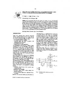
Like a buck converter, the power stage of MC presents current and voltage stiff terminal properties when viewed from the source and load respectively. This is shown in Fig. 1.9a where the MC is modeled as appropriate controlled sources. Balanced 3 phase system has been considered which allows analysis on a single phase basis. The controlled sources shown in Fig. 1.9a are composed of fundamental as well as switching frequency ( f s ) components. Hence, the input side has to be interfaced to the input source through ripple filters to ensure only low-frequency interaction at fundamental frequency. Input filter is an essential requirement of this topology for providing a local circulating path to the switching frequency current. Output side filters are also necessary in applications which require a filtered voltage to be applied to the load. At the same time it has to be ensured through design that addition of filters do not degrade performance parameters like voltage regulation, efficiency and size. These place conflicting demands on the choice of filter elements. Moreover, as the basic structure of MC is made of bi-directional switches, the only associated inertial elements in this topology are the filter components. Consequently the filter parameters affect the system dynamics significantly. Input filter design has been discussed in [1–6], where, from cost and weight considerations, single stage LC filter has been found to be the most appropriate topology. Figure 1.9b, c show the widely used input and output filter configurations. It is not possible to control the input current in MC, hence a damping resistor is used for the input filters. Although the set of filter elements (L f , C f ) for a particular resonant frequency is infinite, [2] advocates a maximum C f to ensure minimum leading Input Displacement Factor (IDF) at low loading conditions. However, in a distribution system most of the loads are inductive and hence this should not be a major concern at lighter loads. An exhaustive treatment of input/output filters with focus on reducing electromagnetic interference and common-mode voltages has been provided in [7]. However, most of these have not investigated the comprehensive design of filters in the context of dynamic performance requirements or reliability of commutation hardware. Filter design, considering stability limits detailed in [8, 9], has been discussed in [6]. However, it will be discussed in a subsequent chapter of this book, that with a proper choice of the modelling paradigm, the derived plant has non-minimum phase zeros but minimum phase poles for all operating points.

8

1 Introduction LC− filter Grid

Matrix converter

Cc

Load

Rc

Fig. 1.10 Clamp circuit

Therefore a stable plant is obtained. The relation between filter parameters and nonminimum phase zeros would be detailed and the modifications necessary in filter design will also be discussed.

1.1.1.3

Protection Schemes

Standard protection schemes like overcurrent and overvoltage protection used in any converter are also necessary in MCs. The switches need to be protected in the event of short circuit at input side and open circuit at the output side. Protection for high current during shorting of input terminals can be realized on the gate drivers of the switches themselves. Standard technique like sensing the collector to emitter voltage across an IGBT to detect short circuit can be employed. Interruption of load current, during communication or due to activation of protection circuit following any fault, may result in high voltage at the output side. Normally a diode clamp circuit along with a capacitor (Cc ) and discharging resistor (Rc ) as shown in Fig. 1.10 is used to absorb the energy of inductive load [4]. Design of the clamp capacitor has been presented in [5]. Clamp circuits requiring lesser number of diodes have also been proposed in the same paper. This circuit also protects the MC from overvoltages at grid side. Overvoltage protection using varistors and zener diodes with high blocking capability is reported in [10].

1.1.2 Commutation One of the major hurdles in controlling MCs is switching a load from one input terminal to another without violating the fundamental switching rules. This difficulty in switching can be understood with the example of a two phase to single phase MC feeding an inductive load shown in Fig. 1.11. The bidirectional switch are realized through the CE configuration using discrete IGBTs and diodes. IGBTs in each bidirectional switch (S1 and S2 ) supporting conduction in the forward (towards


9

S1 S1F

v1

S1R

ioF v2

ioR S2F

S2R

S2

Fig. 1.11 2 phase to 1 phase MC

load) or backward are denoted with additional subscripts F and R respectively. Load was initially connected to v1 and a switchover to v2 is required. Now, simultaneous switching of S1 and S2 shorts the input terminals, while sequential switching leads to momentary opening of load terminal. To avoid this a multi-step commutation process based on either output current direction or relative input voltage magnitude [11, 12] becomes necessary. The objectives of these methods are to ensure that the current is not interrupted and at the same time input terminals are not shorted at any instant during the process of commutation. These approaches are detailed in the following subsections.

1.1.2.1

Output Current Direction Based Commutation

Output current direction must be correctly determined for this method to be successful. Figure 1.12a shows the switching sequence from S1 to S2 for forward (i oF ) and reverse (i oR ) direction of i o , respectively. The sequence is shown in terms of switching function of each IGBT. As an example, commutation sequence for i oF is described. Figure 1.12b shows the different stages of commutation in the two phase to single phase MC. IGBTs shown in bolder mark are those which are turned on (gating pulses are provided), while those which are shown in grey shade indicate the turned off IGBTs. Step 1. Step 2.

Step 3. Step 4.

Non conducting IGBT (S1R ) in the outgoing bidirectional switch S1 , is first turned off. Next, the IGBT in the incoming S2 that can support conduction of i oF i.e. S2F is turned on. If v2 > v1 , then natural commutation from S1 to S2 takes place at this stage. S1F is turned off subsequently. If v1 > v2 , then forced commutation from S1 to S2 occurs at this stage. Finally, S2R is turned on.

10

1 Introduction

(a) ioR

ioF

Commutation starts

Commutation starts

S1F(t)

S1F(t)

S1R(t)

S1R(t)

S2F (t)

S2F (t)

S2R(t)

S2R(t)

(b)

S1F

S1R

S1F

1

S1R

1

ioF

v12

ioR

v12

2

2

S2F

S2R

S1F

S2F

S1R

1

S2R

S1F

S1R

1

ioF

v12

ioR

v12

2

2

S2F

S2R

S1F

S2F S1F

S1R

1

S1R

1

ioF

v12

S2R

ioR

v12 2

2

S2F

S2F

S2R

S1F

S1R

1

S1R

1

ioF

v12

S2R

S1F

ioR

v12 2

2

S2F S1F 1

S2F

S2R

S1F

S1R

S1R

1

ioF

v12

S2R

ioR

v12 2

2

S2F

S2R

S2F

S2R

Fig. 1.12 Switching from S1 to S2 based on output current. a Timing diagram. b Stages of commutation

1.1 Overview of 3-Phase Matrix Converter Fig. 1.13 Estimating current direction by sensing the voltage across a bidirectional switch

11 Vcc

i

R

R Vcc

In steady state, both IGBTs in a bidirectional switch are turned-on to allow reversal of current. The commutation process is thus achieved through 4 steps of turn off-onoff-on sequence. Since turning on times of IGBTs are much lower than the turn off duration, the second and third step can be concurrently executed thereby resulting in a three step commutation method. Since the first step involves turning off an IGBT, incorrect current direction measurement would lead to open circuit of the load. During the zero crossovers (ZC) of i o , correctly sensing its direction may become difficult. To overcome this, a method where the direction of i o is derived by measuring voltage across each device has been reported in [13]. Conceptually this amounts to using an arrangement similar to what is shown in Fig. 1.13. The collector voltage of each device is fed to a comparator, whose output state determines the instantaneous current direction. For example, if the direction of current i is downward as shown, the comparator output would be approximately Vcc . Since the device has to block the input line to line voltage in blocking mode, the voltage at input of the comparator has to be clamped to the control voltage level. Hence, the major fraction of the voltage appears across R. So the value of R has to be high enough to restrict the power loss to an acceptable level. Apart from the increased number of components in this method, use of a high R along with unavoidable stray capacitances makes the measurement prone to errors due to the inherent delays involved [14, 15]. 1.1.2.2

Input Voltage Magnitude Based Commutation

This method requires knowledge of the relative magnitudes of input voltages. Figure 1.14a, b shows the switching sequence from S1 to S2 for different polarities of v1 − v2 . For v1 > v2 , the commutation process as shown in these figures is achieved in the following manner. Step 1. Step 2.

S2F is turned on. This activates the conduction path for i oF in S2 , while ensuring that there is no circulation current between the two input phases. S1F is turned off. At this instant, if i o is in forward direction (i o = i oF ), conduction is taken up by S2 i.e. forced commutation takes place here. However, if i o is in the backward direction (i o = i oR ) conduction would still be supported by S1 .

12

1 Introduction

v1 < v2

v1 > v2

(a)

Commutation starts

(a)

Commutation starts

(b)

S1F (t)

S1F (t)

S1R (t)

S1R (t)

S2F (t)

S2F (t)

S2R(t)

S2R(t)

(b) S1F

S1R

S1F

1

S1R

1

ioF ioR

ioF ioR

2

2

S2F

S2R

S1F

S2F S1R

S2R

S1F

1

S1R

1

ioF ioR

2

ioF ioR

2

S2F

S2R

S1F

S2F

S1R

S2R

S1F

1

S1R

1

ioF ioR

2

ioF ioR

2

S2F

S2R

S2F

S1F

S1R

S2R

S1F

1

S1R

1

ioF ioR

2

ioF ioR

2

S2F S1F 1

S2R

S2F

S1R

S1F 1

S2R S1R

ioF ioR

2

ioF ioR

2

S2F

S2R

S2F

S2R

Fig. 1.14 Switching from S1 to S2 based on relative magnitude of v1 and v2 . a Timing diagram. b Stages of commutation


Step 3. Step 4.

13

S2R is turned on. Therefore conduction path for i oR gets activated in S2 and since v1 > v2 , natural commutation occurs for reverse current flow. Finally S2F is turned off.

If the relative voltage magnitudes can be clearly distinguished the first two steps and the third and fourth step can be merged to form a two step sequence. Voltage based commutation starts with a turning on process. Here, the major concern is correct polarity detection of phase to phase input voltage during its ZC. Falsely detecting this polarity would lead to shorting of the two input terminals. The difficulty in detecting the polarity is compounded by the presence of switching frequency ripple component. Around ZC of the line to line voltage the magnitude of its fundamental component is small but the same does not hold for the ripple component. Also it is much more difficult to accurately measure the switching frequency component than the slowly varying fundamental component. This issue has been addressed in various papers on commutation. In [16], an analysis of critical window width around ZC of input line voltages has been provided, based on the magnitude of fundamental component of input voltage and resonant component that appears due to the input filter oscillations. During commutation between two phase voltages lying in this defined window, an intermediate step is introduced where the switch over takes place through the third phase. However the effect of the input switched current which plays the major role behind switching frequency ripple in input voltage has been ignored. In [17], it is shown that with proper zero vector placement for Space vector modulation (SVM) based approaches, safe commutation can be achieved in spite of voltage measurement inaccuracies. This method is restricted to operation within a certain input displacement angle (±θ ◦ ) around voltage ZC, where θ is to be decided on the basis of the specific input ripple voltage measurements for a given hardware. Moreover, as this method depends on minimum duration of zero vectors it is not applicable to all operating points. For all operating regions and in applications requiring wider control of IDF [18, 19], commutation at ZC of line-line voltage is still difficult, particularly at high output current amplitude. There is no guide for conclusively selecting a particular method for an application. However, applications having a high inductance at the output side will have a low switching ripple component in the output current. Therefore it is easier to sense to measure the output current correctly and thus current based techniques may be better suited for such conditions. For applications requiring a regulated sinusoidal output voltage, an output filter becomes necessary. The inductor in this filter which is in series with the output terminals must be small so that the voltage drop is less. Consequently the ripple components of the current would be large and so would be the magnitude of error in measuring it. The applications considered in this work falls in the latter category. Existing input voltage based commutation method is adopted in this work. A closed-form expression of the ripple voltage in the input filter capacitor and error in measurement has been derived. This is used to derive the minimum size of filter capacitor as would be detailed in a subsequent chapter.

14

1 Introduction

+

a b c

vdc

A B C

− Fig. 1.15 Indirect MC

1.1.3 Topology The structure shown in Fig. 1.7 is referred to as the Direct Matrix Converter (DMC). The operational challenges associated with DMC have prompted engineers to find out variants of this basic structure that may simplify some of the operational issues. Figure 1.15 shows a variant of the basic MC topology. This is known as Indirect MC (IMC) [20]. The power processing in this structure is achieved through rectification and inversion process as found in B2B VSIs. Commutation is reported to be simpler than DMCs [20, 21], as the rectifier stage bidirectional switches can be switched when the inverter side is in free wheeling mode. In this condition, commutation at the rectifier side is not constrained by any restriction on the opening of the output terminals and only needs to ensure that the input terminals are never shorted. Since the DC link voltage (vdc ) has to be positive, IDF can be controlled in the range 0.866–1. Reduction of IMC structure leading to varying forms of ‘Sparse Matrix Converters’ has been summarized in [21]. This work is related to power system applications for synchronous systems. In such applications reactive power plays a significant role. Although control of input reactive power has not been attempted in this work, it can be included in future investigations by extending the analysis presented here. Since DMC offers a much wider scope of IDF control than IMC, it has been adopted here. Hence, subsequent discussions are related to DMCs. However since the basic functional feature of both DMC and IMCs are same, discussion related to dynamic model, filter design and modulation applies equally to both topologies.

1.1.4 Modulation A large number of modulation techniques have been reported, dating back to the inception of MC. A few of those, which have been critically evaluated, are discussed here.


15

(b)

vsa vo vsb

vsc

Input voltage envelope and some possible output voltage aveforms (pu)

(a)

1

0.5 input voltage envelope

0

−0.5

−1

0.075

0.08

0.085

0.09

0.095

0.1

Time (s)

Fig. 1.16 a Input voltage. b Output voltage envelope for all 27 switching combinations

(b)

1

Input and target output voltage (pu)

Input voltage (pu)

(a)

v

0.5

o

0 −0.5 −1

0

0.01

0.02

1 0.5 0 −0.5 −1

0

0.5 0 −0.5

cm

cmo

i

−1

0

0.01

Time (s)

0.02

(e)

1

Input and reshaped target output voltage (pu)

(d)

1

Reshaped target output voltage (pu)

Target output and common mode voltages (pu)

(c)

0.01

0.02

Time (s)

Time (s)

0.5 0 −0.5 −1

0

0.01

0.02

Time (s)

1

0.5

0

−0.5

−1

0

0.01

0.02

Time (s)

Fig. 1.17 a Input voltages. b Input and target output voltages. c Target output voltages along with common mode voltages. d Reshaped target voltages. e Input along with reshaped target output voltages

1.1.4.1

Direct Transfer Function Based Approach

One of the earliest papers [22] known to provide a rigorous analysis of a 3-phase MC demonstrated this approach (Fig. 1.16). This method derives the low frequency modulation signals directly from the reference and input voltages. In the first algorithm [22] the envelope of output voltage waveform to be synthesized must remain within the input voltage envelope at all instants of time. Consequently, as shown in Fig. 1.17a, the maximum achievable output voltage (vo ) amplitude is 0.5 times of the input. The performance was significantly improved in the second algorithm [23] where the maximum 0.866 voltage gain ratio could be reached. The essence of the second algorithm is explained with the help of Fig. 1.17b–e. Figure 1.17b shows the input and target output voltages

16

1 Introduction

whose amplitude are 0.866 times of the input. The output waveform is observed to exceed the input waveform envelope at some intervals. By appropriately adding common mode (cm) terms, the second algorithm reshapes the target voltage envelope to completely fit into the input envelope. Figure 1.17c shows the third harmonic cm components for input (cm i ) and output (cm o ) which are added on to the target output waveform. Figure 1.17d shows the reshaped target waveforms, the envelope of which is now completely enclosed by that of the input waveform, as shown in Fig. 1.17e. Since the load and supply neutrals are usually isolated and the cm terms disappear from the line to line voltages, addition of these low frequency terms are justified. Denoting the input and target output voltage amplitude and frequency as Vî , Vô∗ , and ωi , ωo respectively, the described procedure is equivalent to generating the output voltage references as [23], ⎡

⎡ ⎡ ⎡ ⎤ ⎤ ⎤ ⎤ cos(ωo t) cos(ωo t) cos(3ωi t) cos(3ωo t) ∗ ˆ ˆ V V i o ⎣ cos(3ωi t) ⎦ − ⎣ cos(3ωo t) ⎦ VôR ⎣ cos(ωo t − 120◦ ) ⎦ = Vô∗ ⎣ cos(ωo t − 120◦ ) ⎦ + 4 6 cos(ωo t + 120◦ ) cos(ωo t + 120◦ ) cos(3ωi t) cos(3ωo t)

cm i

cm o

(1.4) If the output load angle (φ L ) can be measured, IDF can also be controlled using the second algorithm. The same maximum voltage gain and IDF control can be achieved by other modulation methods without the necessity of measuring φ L and therefore having a relatively simple hardware realization. They are described in the following section.

1.1.4.2

Space Vector Modulation (SVM)

The power stage of MC can be viewed [24] as a cascaded rectifier-inverter stage coupled by a fictitious DC link as shown in Fig. 1.18. SVM based on this decoupled construct allowing control of IDF has been described in [25]. This method is referred

va a

iAB

vc

vb b

iCA iBC

c

A

B

p n Rectifier

Fig. 1.18 Decoupled rectifier-inverter construct

Inverter

C


17

(b) v

a

(a) vc

vb

va

vc

vb

a

b

c

iCA iB C

iAB

A

iAB a

b

c

A

B

C

p

B

iCA

iB C C

n

Fig. 1.19 Mapping the switching functions

in this book as Indirect space vector modulation (ISVM). Here, the duty ratios of the switches for individual stages are initially calculated and then combined on the basis of instantaneous active power balance between input and output. Thereafter, the switching functions for the twelve switches are mapped to the nine 4Qsws MC structure. An example of this mapping from the 12 to 9 switch structure is shown in Fig. 1.19a, b. Suppose the input terminal a in the decoupled structure needs to be connected to output terminals A and C, while terminal b to output terminal B as shown in Fig. 1.19a. The corresponding switches which need to be closed in the 9 switch structure are shown in Fig. 1.19b. A maximum voltage gain of 0.866 for unity IDF is attainable with ISVM. Hardware realization of ISVM is simpler than direct approaches and knowledge of φ L is not required for IDF control. Moreover, space vector based schemes offers substantial freedom in choosing the switching sequence which can be used for reducing common mode voltage at the output [26], output current ripple [27], reducing switching losses [28] etc. These features make SVM one of the most widely adopted modulation method in MCs. The basic working principle of ISVM has been briefly discussed later in this book.

1.1.4.3

Other Pulse Width Modulation (PWM) Based Methods

One of the often stated disadvantages of SVM lies in the use of look-up tables for hardware realization. This has been the primary inspiration for alternate PWM methods like [29] where cm terms are added to modulation signals in order to achieve a voltage gain of 0.866. Control of IDF is also possible in this scheme. Another carrier based method [30] emulates the input line to line voltages as the DC link voltage of an inverter and by doing so tries to extend modulation strategies for VSI to MC. The method proposes to use two input line to line voltage as the imaginary DC link voltage over a switching cycle. The input voltages are denoted as Vmax , Vmed and Vmin based upon their relative magnitudes, as shown in Fig. 1.20. The switching period Ts is divided into two parts T1 and T2 depending on the input voltage angle.

18

1 Introduction Voltage (pu)

Fig. 1.20 Describing the discontinuous carrier signals [30]

Vmax C2

C1

Time (s)

Vmed Vmin T1

T2 TS

Now for the two separate parts of the switching cycle, two carriers (C1 and C2 ) are defined as the difference between the values of input voltages. The argument behind using two carriers, is, utilization of all three input voltages during a switching period [30]. If two inputs are only used, one of the input phase currents would remain zero thereby leading to higher input current distortion. A voltage gain of 0.866 in the linear modulation region and unity IDF is ensured with this method. The PWM based methods are gradually becoming an active area of research. The performance in terms of voltage gain and controllable IDF has been proven to be equivalent to SVM methods. However the superiority or equivalence of these in context of the flexibility shown by SVM schemes in choosing and placing the zero vectors is yet to be established.

1.1.4.4

Discrete Methods Based on Predictive Model

Modulation methods based on discrete models have been a very actively researched topic in the last decade. These methods use discrete-time models of the load, filter and converter to predict behaviour of variables like load current, reactive power etc. For example, if the objective is to control the output current (i o ), its value at k + 1th sampling instant is first computed using the predictive models for all valid switching states. The resulting absolute error between the reference and predicted values for a single valid switching state can be represented as i o (k + 1) = i o∗ (k + 1) − i op (k + 1) ,

(1.5)

where ∗ and p denote reference and predicted values respectively. Subsequently, the state that gives minimum i o (k + 1) is chosen as the k + 1th switching state. However, as no current feedback is used, this may cause unchecked deviation of actual current. The strength of the method lies in its flexibility to address multiple


19

control objectives. An example of this was reported in [31], where the objective was to control i o and minimize input reactive power qs . A quality function (Q G ) was defined as (1.6) Q G = W 1 · i o (K + 1) + W 2 · qs (K + 1), where W 1, W 2 are weighting functions. An analytical approach of choosing the weighting functions is yet to be reported. On basis of a particular set of W 1 and W 2, Q G is calculated for all the 27 valid switching states of MC. Thereafter the state resulting in minimum Q G is selected at the next switching instant. Applications of this predictive model based approach for different control objectives are summarized in [32]. Keeping aside the obvious concern regarding the accuracy of the predictive models, on-line computation of Q G for all valid switching states would increase the computational burden to a great extent. Superiority of this technique over the performance obtained with SVM approaches has not been established yet [32].

1.1.5 Dynamic Model for Controller Design Tight coupling between the input and output side of MC complicates controller design, particularly for applications requiring high bandwidth. Hence, for stable operation, a proper control scheme based on a tractable dynamic model becomes necessary—an area, which has not received sufficient attention. This has been acknowledged in [33] which presents a dynamic model for MC used as an interface between high speed micro turbine generator and the utility grid. The model is developed using state matrices, which is subsequently utilized for design of active and reactive power control. State feedback approaches based on eigenvalue analysis has been used in [34] for voltage sag mitigation, another application which demands high dynamic performance. With available tools like MATLAB control toolbox, designing controllers using state matrices is not difficult and desired dynamic performance is guaranteed provided the system is well modeled. But these methods provide little insight into the system as associating the eigenvalues, or critical dynamic behavior, with specific physical elements becomes increasingly difficult with higher order systems. In the context of stable operation of MCs, [8, 9, 35–38] have reported and analyzed existence of a throughput power limit (Plim ) for stable operation. In all these studies, for output voltage control, the reference V¯o∗ is obtained treating the output filter and the load as plant. Subsequently the modulation signals are essentially computed as m¯ =

V¯o∗ , V¯in

(1.7)

20

1 Introduction

where V¯in is voltage vector of the input voltage vin (vc f ) applied at the input terminals shown in Fig. 1.9a, b. Although m¯ is not extracted exactly through a scalar division as it appears in (1.7), the conceptual basis is essentially same. This method is sometimes referred as feed forward compensation of input voltages [8]. Plim is prescribed by investigating the input side of MC assuming constant active power transfer through it. Investigation of how filtering V¯in affects the system eigenvalues has been reported in [36]. Examination of how sampling delays in measuring V¯in affects Plim has been detailed in [8, 9] considering constant output power. More recently [38] has proposed use of the source voltage i.e. vs in Fig. 1.9b in place of vc f which improves the stability limit for grids having a low source impedance. A detailed discussion on the dynamic model and appropriate controller design has been provided later in this book chapter.

1.2 Motivation and Objectives Out of the different research tracks highlighted in the last section, major effort has been spent in investigating modulation algorithms that can extract the optimal performance out of MC in terms of voltage gain, IDF control, relative ease of hardware realization, switching losses etc. This has been followed by devising reliable commutation and protection strategies, alternative topologies with reduced number of switches in certain cases where unidirectional flow of power is required, input filter design etc. One of the lesser investigated area has been the development of a dynamic model that provides a physical insight into the system. From the applications perspective, although MC is perceived as an alternative to B2B VSI (DAB), research efforts has been largely confined to motor/drive. The last decade have witnessed an emerging academic interest in using MC for power system applications. For example, it has been reported to be used as a reactive power compensator [18, 19], voltage sag compensator [34], regulated utility power supply [39], Unified power flow controller [40] to name a few. A major motivation of writing this book is to introduce to the reader the considerations for using the MC for synchronous power system applications. Two typical applications were chosen for investigation—regulated voltage supply and voltage sag mitigation. Of course, several research publications have reported MC based solutions, along with dynamic model and control techniques, for interfacing with utility power systems. Section 1.1.5 of this book shows that some of these approaches, which are either based on feed forward compensation of input voltages or on state feedback based schemes, have specific limitations. Some reports, e.g. [34], incorporate an additional flywheel energy storage which negates the high power density advantages of the MC. Hence, the broad aim of this book is categorized into the following objectives. 1. Complexity of control has been widely acknowledged to be one of the major reasons for the low industrial acceptance of MC, even after three decades of

1.2 Motivation and Objectives

21

intensive research. Control may become more difficult as one moves out of the motor/drives domain to power system applications, which demand faster dynamic performance. For a tightly coupled input-output unit like the MC, the system designer cannot take an independent approach towards design of sub components like filter and controller, without addressing common constraints that bind both. A dynamic model that helps to identify such common links and also aid the physical understanding of the system is presented in this book. So development of a tractable dynamic model by which the stated concerns can be addressed was set to be the first objective of the work. 2. The next goal was to obtain a design guideline for filters which should also take into consideration the constraints that emerge from the dynamic model and sizing of passives for reliable commutation. 3. Once the first two targets were achieved, controller design naturally became the third objective. Given that a recurring argument against using MC has been the difficulty of control, emphasis was given on finding a control scheme that is easily realizable. 4. Experimental validations of the analytical claims was set as the final objective.

1.3 Assumptions and Scope The analysis presented in this book uses a set of assumptions, which are routinely made in MC analysis but are stated nevertheless for clarity. This also helps to delineate the scope of this book, which are listed below to enable correct evaluation of the material presented here. • Plant model is derived assuming 3 phase balanced system. Harmonic distortions in supply voltage has not been considered. • Modelling is confined to synchronous applications. • Ideal converter and filter elements have been assumed. • Dynamics of Phase lock loop (PLL) have not been considered. • Harmonic analysis of MC has not been carried out. • For voltage sag mitigation a 3 wire linear load is considered thereby removing any possibility of zero sequence component in load.

1.4 Layout of the Book The rest of the book is structured in the sequence the objectives were described. The next chapter i.e. Chap. 2 describes the development of linearized plant model based on the low frequency gain of MC. The same model is used for the investigation of the plant for non-minimum phase poles/zeros. Chapter 3 presents the filter design approach where the different performance criteria are set in the process to

22

1 Introduction

find an acceptable solution set for filter parameters that satisfy all of them. Relevant experimental results are presented. The next two chapters deal with the application aspects where the design techniques have been applied. In Chap. 4, a controller design approach for an application requiring regulated 3 Phase sinusoidal voltage is described. Experimental results are presented. The control design approach is then extended with appropriate modifications in the next chapter where MC is used as a voltage sag mitigating device. Chapter 5 discusses symmetrical and asymmetrical voltage sag mitigation using MC for linear loads. Experimental results are presented. Some critical observations based on the presented material are summarized in Chap. 6 along with some observations of the authors.

Chapter 2

Low Frequency Dynamic Model

Like other converters in the switched mode power converter family, operation of matrix converters involves two significant frequency components. These are the fundamental frequency and the switching frequency. The fundamental frequency component is associated with power transfer while the switching component is a byproduct of the operation. If these switching components are injected into the grid side or to the load side it would lead to undesirable consequences and thus it is necessary to filter them. The filtering process has been discussed in detail in a later chapter. For this chapter, it is sufficient to have the understanding that low pass filters are realized by passive elements in these converters. For a given power level, the size of these filter components reduces as the switching frequency becomes higher. Hence a large difference between the switching frequency and the fundamental component is always preferable as it helps to achieve effective filtering with smaller components size. The switching frequencies are in the order kHzs, or tens of kHzs, a number which depends upon the rated power handling capacity of the converter. On the other hand, the order of the fundamental component is usually tens of Hertz. For any well designed converter, the switching frequency component in the output variables are negligible compared to the fundamental frequency component. Therefore, while deriving a model which represents the dynamic behaviour of the converter the high switching frequency component can be neglected without any loss of accuracy in modelling. Thus the control scheme of MC or for many other SMPCs has to be devised such that the fundamental frequency component and low frequency harmonic components can be processed with a desired degree of accuracy. This chapter presents an analysis of the linearized low frequency model of MC, where it has been used as a 3-phase regulated sinusoidal voltage supply. The objectives of all modulation techniques for MC are attaining the desired—amplitude, phase and frequency of the output voltages and IDF at the input side. In the first section of this chapter, the modulation technique adopted in this work is briefly discussed to describe the low frequency gain of MC. It has been subsequently used to develop the linearized dynamic model in Sect. 2.2 from where the plant transfer function matrix © Springer Nature Singapore Pte Ltd. 2017 A. Dasgupta and P. Sensarma, Design and Control of Matrix Converters, Energy Systems in Electrical Engineering, DOI 10.1007/978-981-10-3831-0_2

23

24

2 Low Frequency Dynamic Model

is derived. In Sect. 2.3 it is demonstrated how the system poles/zeros are affected by input voltage, input displacement factor, throughput power and parameters of the input filter. In the process it is found that based on the operating points, right half zeros may emerge in the control to output transfer functions beyond a critical level of input power.

2.1 Low Frequency Gain of 3-Phase MC The phase to input side neutral voltages applied to the converter i.e. the voltages at terminals a, b and c with reference to the input neutral shown in Fig. 2.1 are represented as ⎡

⎤ ⎡ ⎤ va cos(ωi t − ϕc ) ⎣ vb ⎦ = vcf (3) = Vˆc f ⎣ cos(ωi t − ϕc − 120◦ ) ⎦ . vc cos(ωi t − ϕc + 120◦ )

(2.1)

These voltages appear across the input filter capacitor C f depicted in the perphase diagram shown in Fig. 1.9b and reproduced in Fig. 2.2. MC allows control on the magnitude, frequency and phase of the output voltage and IDF. Let the desired output voltages, referred to output neutral n, be described as ⎡

v∗ on

(3)

⎤ ⎡ ⎤ v ∗An cos(ωo t + ϕo ) = ⎣ v ∗Bn ⎦ = Vô ⎣ cos(ωo t + ϕo − 120◦ ) ⎦ , ∗ vCn cos(ωo t + ϕo + 120◦ )

(2.2)

ni

Fig. 2.1 Schematic of a 3-ph MC

vsa

vsb

vsc

Input filter

ia

a

ib b ic

c

A

B

iB C

iC

Output filter

iA

n

2.1 Low Frequency Gain of 3-Phase MC

25

Fig. 2.2 Input side equivalent circuit for the per-phase system

Rd

is Lf

vs

C

f

grid

vcf

iin

input filter

where ∗ indicates reference signal. The corresponding line to line voltages are ⎤ ⎡ ∗ ⎤ ⎡ ⎤ v AB cos(ωo t + ϕo + 30◦ ) v ∗An − v ∗Bn √ ∗ ⎦ v∗ oL = ⎣ v ∗Bn − vCn = ⎣ v ∗BC ⎦ = 3Vô ⎣ cos(ωo t + ϕo + 30◦ − 120◦ ) ⎦ . ∗ ∗ vCn − v An vC∗ A cos(ωo t + ϕo + 30◦ + 120◦ ) (2.3) Indirect space vector modulation (ISVM) [25] method has been adopted in this work to synthesize the desired voltage output. The basic principle of this method is discussed in the following section. ⎡

(3)

2.1.1 Indirect Space Vector Modulation (ISVM) Approach In ISVM technique the 9 bidirectional switch MC structure is conceptually decoupled into an equivalent cascaded chain of fictitious current and voltage source converters (CSC and VSC) as shown in Fig. 2.3. The imaginary DC link voltage and current i.e. Vdc and Idc are treated as sources for the VSC and CSC parts respectively. The duty cycle of each switch in the 9 bidirectional switch MC structure is calculated in two stages. In the first stage, the duty cycles are calculated separately for each converters of the decoupled construct using conventional space vector modulation (SVM)

va a

n

vc

vb

Fictitious DC link

b

c

+

Idc

A

B

C

Vdc − Current Source Converter

Voltage Source Converter

Fig. 2.3 Decoupled current and voltage source converter construct

26


approach. In the next stage, the individual duty cycles are combined based on instantaneous active power balance between the input and output sides. The duty cycle of the 12 switch fictitious CSC–VSC structure can be then directly mapped to the 9 bidirectional switch MC topology. To illustrate this procedure, the VSC part is considered first, where the reference line to line voltages are used to define the vector

2 ∗ v AB + v ∗BC e j2π/3 + vC∗ A e− j2π/3 . (2.4) 3 √ Here the constant multiplier 2/3 ensures power invariant transformations. Sub¯ ∗oL is obtained as stituting the line voltages from (2.3) in (2.4), V ¯ ∗oL V

=

¯ ∗oL = √3 Vô e j (ωo t+ϕo +30◦ ) . V 2

(2.5)

Referring to Fig. 2.3, there are 8 valid switching combinations by which the output terminals of the VSC can be connected to the fictitious DC link. Here, the term valid combinations refers to those which ensure that any output terminal is never left open. The line voltages corresponding to each of these combinations are used to create the vector ¯ oL = 2 v AB + v BC e j2π/3 + vC A e− j2π/3 . (2.6) V 3 Applying (2.6) to each of the 8 combinations result in stationary vectors (SV) which are sometimes also referred to as switching state vectors. These are tabulated in Table 2.1 and also shown in Fig. 2.4a.

Table 2.1 Switching state vectors for the VSC ¯ oL V A B C

2

+

–

–

3

+

+

–

3

–

+

–

3

–

+

+

3

–

–

+

3

+

–

+

3

–

–

–

+

+

+

2 2 2 2 2

2 3

√ 2Vdc ∠30◦ √ [0 + Vdc e j2π/3 − Vdc e− j2π/3 ] = 2Vdc ∠90◦ √ [−Vdc + Vdc e j2π/3 + 0] = 2Vdc ∠150◦ √ [−Vdc + 0 + Vdc e− j2π/3 ] = 2Vdc ∠210◦ √ [0 + −V pn e j2π/3 + V pn e− j2π/3 ] = 2Vdc ∠270◦ √ [V pn − V pn e j2π/3 + 0] = 2Vdc ∠330◦ [Vdc + 0 − Vdc e− j2π/3 ] =

[0 + 0 + 0] = 0

Stationary vectors V1 V2 V3 V4 V5 V6 V0


27

(a)

V2 * axis of vBC

III

V3

sector I

V0

IV

ωo

V4

V

(b)

V1

II

VI

Vβ

ω o t + ϕo + 30o = 0

*

VoL

Vβdβ

* axis of vAB

* VoL

θSV

Vαdα

V6

Vα

* axis of vCA

V5 ∗

∗

¯ oL . b Synthesizing V ¯ oL Fig. 2.4 a Output voltage stationary vectors and V

It is evident that there are 6 sets of SVs with non zero magnitude having distinct spatial orientation and 2 sets of SVs with zero magnitude. The objective of SVM is ¯ ∗oL , in a time-averaged sense, over a switching period (TS ), by using to synthesize V the available SVs as

TS

TS ¯ ∗oL dt = ¯ oL dt. V V (2.7) 0

0

Since the switching frequency ( f S ) is much higher than the fundamental frequency, ¯ ∗oL practically behaves like a stationary vector over a single switching period. So V with appropriate scaling, many combinations of SVs can be used to synthesize the ¯ ∗oL . However, using two adjacent SVs leads to minimum numtarget voltage vector V ¯ oL is ¯ ∗oL − V ber of switching. Additionally, the instantaneous voltage deviation V lowest, which ensures minimum current ripple in the inductors connected to the output terminals. The adjacent SVs, Vα and Vβ , are shown in Fig. 2.4b trailing and ¯ ∗oL and Vα . Over ¯ ∗oL respectively. θ SV is the instantaneous angle between V leading V ¯ ∗oL implies a constant θ SV . a single switching period TS , assumption of a stationary V ∗ ¯ oL can be synthesized as Therefore, V ¯ ∗oL = Vα Tα + Vβ Tβ V TS TS = Vα dα + Vβ dβ .

(2.8)

Applying properties of triangle, ∗

¯ oL | |Vβ dβ | |Vα dα | |V = . = sin 120◦ sin(60◦ − θ SV ) sin(θ SV )

(2.9)

28

2 Low Frequency Dynamic Model ∗

¯ oL is in sector I Table 2.2 Line voltages, when V During d6 (dα ) During d1 (dβ )

ON time A

B

C

dα TS

+

–

+

dβ TS

+

–

–

v AB

v BC

vC A

−→

Vdc

−Vdc

0

−→

Vdc

0

−Vdc

Using (2.5), Table 2.1 and (2.9), dα and dβ are determined as √ 3 Vô dα = sin(60◦ − θ SV ) = m v sin(60◦ − θ SV ), Vdc √ 3 Vô dβ = sin(θ SV ) = m v sin(θ SV ). Vdc

(2.10)

¯ ∗oL be considered to be lying in sector I. Here Vα = V6 and As an example, let V Vβ = V1 . Using Table 2.1, the line voltages corresponding to the two duty cycles are shown in Table 2.2. Using (2.10) and Table 2.2, the average value of the synthesized output voltages ¯ oL is in sector I, are obtained as over TS , when V ⎤ ⎡ ⎤ ⎡ ⎤ dα + dβ cos(θ SV − 30◦ ) v AB = ⎣ v BC ⎦ = ⎣ −dα ⎦ Vdc = m v ⎣ − sin(60◦ − θ SV ) ⎦ Vdc . vC A −dβ − sin(θ SV ) ⎡

voL (3)

(2.11)

¯ oL is in sector I, θ SV can be evaluated in terms of Again from Fig. 2.4a, b, when V output voltage frequency and phase as θ SV − (ωo t + ϕ0 + 30◦ ) = 30◦ =⇒ θ SV = ωo t + ϕo + 60◦ .

(2.12)

Substituting θ SV from (2.12) in (2.11), the output voltages can be expressed as ⎡

voL (3)

⎤ cos(ωo t + ϕo + 30◦ ) = m v ⎣ cos(ωo t + ϕo + 30◦ − 120◦ ) ⎦ Vdc = mv Vdc , cos(ωo t + ϕo + 30◦ + 120◦ )

(2.13)

mv

where mv represents the low frequency gain matrix of the VSC part. Using Table 2.1, Fig. 2.4a, b, the ratio of the output voltages to Vdc and θ SV in terms of output voltage frequency and phase for sectors II to VI are tabulated in Table 2.3. For all the sectors, evaluation of the average value of the synthesized output voltages results in the expression described by (2.13).


29

Table 2.3 Ratio of line voltages to Vdc , θ SV for sectors II to VI v AB Vdc v BC Vdc vC A Vdc

θ SV

−dα − dβ −dα dβ dα + dβ dα

ωo t ωo t ωo t ωo t ωo t

Sector II Sector III Sector IV Sector V Sector VI

dα −dβ −dα − dβ −dα dβ

dβ dα + dβ dα −dβ −dα − dβ

Table 2.4 Switching state vectors for CSC + – a b b c c a a b c

c c a a b b a b c

I¯in √ 2Idc ∠30◦ √ 2Idc ∠90◦ √ 2Idc ∠150◦ √ 2Idc ∠210◦ √ 2Idc ∠270◦ √ 2Idc ∠330◦ 0

+ ϕ0 + ϕ0 − 60◦ + ϕ0 − 120◦ + ϕ0 − 180◦ + ϕ0 − 240◦

State vectors I1 I2 I3 I4 I5 I6 I0

The low frequency gain matrix of the CSC part is derived in a similar manner. If ϕi is the desired input displacement angle, the desired input currents are then represented as ⎡

i∗in (3)

⎤ ⎡ ⎤ i a∗ cos(ωi t − ϕc − ϕi ) = ⎣ i b∗ ⎦ = Iîn ⎣ cos(ωi t − ϕc − ϕi − 120◦ ) ⎦ , i c∗ cos(ωi t − ϕc − ϕi + 120◦ )

(2.14)

and therefore the target input current rotating vector is ∗ I¯in

=

2 ∗ (i + i b∗ e j2π/3 + i c∗ e− j2π/3 ) = 3 a

3 ˆ j (ωi t−ϕc −ϕi ) . Iin e 2

(2.15)

The valid switching states along with the SVs are tabulated in Table 2.4. Figure 2.5 shows the SVs of the CSC construct. The duty cycles for the switches of the fictitious CSC part are determined in the same manner as their VSC counterparts. They are dμ =

Iîn Iîn sin(60◦ − θ S I ) = m i sin(60◦ − θ S I ) & dγ = sin(θ S I ) = m i sin(θ S I ). Idc Idc

(2.16)

30

2 Low Frequency Dynamic Model ∗

Table 2.5 Input currents when I¯in is in sector I During d6 (dμ ) During d1 (dγ )

+

–

a

b

a

c

ia

ib

ic

−→

Idc

−Idc

0

−→

Idc

0

−Idc

Fig. 2.5 Input current vectors

I2 I3

III

I0

IV

I4

I1

II

sector I

VI

V

ωi t ϕc ϕ i = 0

I6

I5 ∗ Here, θ S I , μ, γ are analogous to θ SV , α, β in Fig. 2.4b. When I¯in is in sector I, where Iμ = I6 and Iγ = I1 , the input currents are shown in Table 2.5. Additionally, for sector I, θ S I can be expressed as

θ S I = ωi t − ϕc − ϕi + 30◦ .

(2.17)

Using (2.16), (2.17) and Table 2.5, the synthesized input phase currents are ⎡

iin (3)

⎤ ⎡ ⎤ ⎡ ⎤ ia dμ + dγ cos(ωi t − ϕc − ϕi ) = ⎣ i b ⎦ = ⎣ −dμ ⎦ Idc = m i ⎣ cos(ωi t − ϕc − ϕi − 120◦ ) ⎦ Idc ic −dγ cos(ωi t − ϕc − ϕi + 120◦ ) = mi Idc ,

mi

(2.18) where mi represents the low frequency gain matrix of the CSC part. The ratio of the input current to Idc and θ S I in terms of input current frequency and phase for sectors II–VI are tabulated in Table 2.6. From the discussion based on separate CSC and VSC structure, it seems that both v∗oL (3) and i∗in (3) can be synthesized independently. This would imply that the duration of active vectors in one converter, i.e. those corresponding to active power flow, can be independent of the active power flow duration in the second converter. However this is not possible. As an example, a zero vector for VSC means all 3 output phases are connected to the same DC link terminal—resulting in zero Idc . Hence, a nonzero


31

Table 2.6 Ratio of input currents to Idc , θ S I for sectors II–VI i a Idc i b Idc i c Idc Sector II

dμ

dγ

−dμ − dγ

Sector III

−dγ

dμ + dγ

−dμ

Sector IV

−dμ − dγ

dμ

dγ

Sector V

−dμ

−dγ

dμ + dγ

Sector VI

dγ

−dμ − dγ

dμ

θS I ωi t − ϕc − ϕi 30◦ ωi t − ϕc − ϕi 90◦ ωi t − ϕc − ϕi 150◦ ωi t − ϕc − ϕi 210◦ ωi t − ϕc − ϕi 270◦

− − − − −

∗ I¯in cannot be synthesized during this period. Therefore, at a given instant of time, it is not possible to have an active vector in one converter and a zero vector in the other one. This is where the second stage of duty cycle computation begins as described in the following. Absence of any intermediate storage element in the power stage of MC implies that instantaneous active power at the input and output side must be same. This power balance necessarily requires that the active vector states of VSC and CSC must be chosen at the same instant and applied for exactly the same duration. This requires combining the gain matrices of the VSC and CSC parts. If Pin be the throughput power, then using (2.18),

Pin (3) vcf =⇒ Vdc = {mi }T vcf (3) . Vdc (2.19) Subsequently, substituting Vdc in (2.13) by using (2.19), the voltage gain relation is obtained as (2.20) voL (3) = mv {mi }T vcf (3) . Pin = {iin (3) }T vcf (3) = {mi }T Idc vcf (3) = {mi }T

Hence mv {mi }T is the input phase to output line voltage low frequency gain matrix. Using (2.13) and (2.18), this gain is evaluated as ⎡

mv {mi }T =

⎤⎡ ⎤T cos(ωo t + ϕo + 30◦ ) cos(ωi t − ϕc − ϕi ) m v m i ⎣ cos(ωo t + ϕo + 30◦ − 120◦ ) ⎦ ⎣ cos(ωi t − ϕc − ϕi − 120◦ ) ⎦ , cos(ωo t + ϕo + 30◦ + 120◦ ) cos(ωi t − ϕc − ϕi + 120◦ ) m

(2.21) where m is commonly referred to as modulation index. The output voltage referred to output neutral n, can thus be represented as von (3) = m(3) vcf (3) ,

(2.22)

32


where, the input-output phase voltage gain matrix m(3) is obtained from (2.21) as ⎡ ⎤⎡ ⎤T cos(ωo t + ϕo ) cos(ωi t − ϕc − ϕi ) √ m(3) = (m/ 3) ⎣ cos(ωo t + ϕo − 120◦ ) ⎦ ⎣ cos(ωi t − ϕc − ϕi − 120◦ ) ⎦ . cos(ωo t + ϕo + 120◦ ) cos(ωi t − ϕc − ϕi + 120◦ ) (2.23) From power balance and gain relationship of (2.22), T iin (3) = m(3) io (3) .

(2.24)

Instantaneous input-output power balance also implies that 3 ˆ ˆ 3 Vc f Iin cos ϕi = Vô Iô cos ϕoL , 2 2

(2.25)

where, ϕoL is the output displacement angle and Iô is the amplitude of the output current (i o ). So for a given v∗on (3) , load and vcf (3) , it is not possible to independently control ϕi and Iîn . Using (2.25) along with m v and m i defined in (2.10) and (2.16) respectively, the modulation index m is evaluated as √ m = mv mi =

3 Vô Vdc

Iîn Idc

√ =

3 Vô Iîn Vô . = √ Pin 3 ˆ Vc f cos(ϕi ) 2

(2.26)

Using (2.25) and (2.26), the magnitude of the input output variables are related as √ Vô =

√ 3 ˆ 3 ˆ ˆ m Vc f cos(ϕi ) and Iin = m Io cos(ϕoL ). 2 2

(2.27)

¯ ∗oL and I¯∗in are in sector I of their corresponding hexagons, using Now, when both V (2.11) and (2.18), the input phase to output line voltage low frequency gain matrix is obtained as ⎡

⎤⎡ ⎤T dα + dβ dμ + dγ mv {mi }T = ⎣ −dα ⎦ ⎣ −dμ ⎦ . −dβ −dγ Therefore the average output line voltages over a switching cycle Ts are

(2.28)


33

⎤ ⎡ ⎤⎡ ⎤T ⎡ ⎤ dα + dβ v AB dμ + dγ va ⎣ v BC ⎦ = ⎣ −dα ⎦ ⎣ −dμ ⎦ ⎣ vb ⎦ vC A −dβ −dγ vc ⎡

⎡

⎤ dμ (dα + dβ )(va − vb ) − dγ (dα + dβ )(vc − va ) ⎦ −dα dμ (va − vb ) + dα dγ (vc − va ) =⎣ −dβ dμ (va − vb ) + dβ dγ (vc − va ) ⎡

⎡ ⎤ ⎤ dμ (dα + dβ ) −dγ (dα + dβ ) ⎦ vca . dα dγ = ⎣ −dα dμ ⎦ vab + ⎣ −dβ dμ dβ dγ

(2.29)

Thus there are four combinations of duty cycles dα dμ , dα dγ , dβ dμ and dβ dγ corresponding to the active states Vα Iμ , Vα Iγ , Vβ Iμ and Vβ Iγ . Using (2.10), (2.16) and (2.26), the duty cycle for the active state Vα Iμ is √

3 Vô Iîn sin(60◦ − θ SV ) sin(60◦ − θ S I ) Vdc Idc = m sin(60◦ − θ SV ) sin(60◦ − θ S I ).

dα dμ =

(2.30)

Similarly, the following are derived dα dγ = m sin(60◦ − θ SV ) sin(θ S I ), dβ dμ = m sin(θ SV ) sin(60◦ − θ S I ), dβ dγ = m sin(θ SV ) sin(θ S I ).

(2.31)

The input-output connections over a switching period in the decoupled construct and the corresponding connections in the actual matrix topology are shown in Table 2.7.

Table 2.7 Mapping from CSC VSC construct to 9 Qsw MC CSC VSC construct ON time dα dμ TS dβ dμ TS dα dγ TS dβ dγ TS

A + + + +

B – – – –

C + – + –

+ a a a a

– b b c c

3 Ph MC A a a a a

B b b c c

C a b a c

34


2.1.1.1

Transformation of 3 Phase Variables in abc Domain to dq Domain

In this analysis the modelling of the system has been carried out in a synchronously rotating (dq) domain. The advantage of working in the dq domain are that the fundamental frequency components of all variables which were varying sinusoidally in abc domain are transformed to time invariant quantities in steady state. This greatly simplifies the task of analysis and controller design. The 3 Ph variables of (2.22) in abc domain are transformed to a synchronously rotating (dq) frame using the transfer matrix ⎡ cos(ωT t) cos(ωT t − 120◦ ) cos(ωT t + 120◦ ) ⎤ 2⎣ − 120◦ ) sin(ωT t √ + 120◦ ) ⎦ , sin(ω T= √T t) sin(ωT t √ 3 1/ 2 1/ 2 1/ 2

(2.32)

in the following manner ⎡

von

⎡ ⎤ ⎤ vond vc f d = ⎣ vonq ⎦ = Tvon (3) = Tm(3) T−1 Tvcf (3) = m ⎣ vc f q ⎦ = m vcf . von0 vc f 0

(2.33)

Here, ωT t is estimated by a PLL locked to the phase—a of the point of common coupling (PCC). For synchronous applications, ωT = ωo = ωi . Since balanced 3phase system has been considered, the zero sequence components can be neglected. The output-input voltage relationship in (2.33) gets modified to

von

v = ond vonq

vc f d = m vcf = m , vc f q

(2.34)

where, the gain matrix m is obtained using (2.22), (2.23) and (2.32), as √ m=

3 cos ϕo md cos θi sin θi = cos θi sin θi . m sin ϕ m 2 o q

(2.35)

θi = ϕi + ϕc .

(2.36)

Here, m d and m q allow complete control on the voltage gain of MC and θi on the input displacement angle. The input currents are obtained as iin = mT io .

(2.37)


vin

m

35

von

mT

io

iin

Fig. 2.6 Low frequency gain of MC

This concludes the discussion on the low frequency gain of MC. The ‘black box’ model of the low frequency gain of MC is shown in Fig. 2.6. Dynamic modelling is discussed in the next section.

2.2 Linearized Model Figure 2.7 shows the single phase equivalent of the overall system where the source impedance has been modelled as an inductance L s . P represents the PCC. An output ripple filter is also necessary to attenuate the switching frequency components in the voltage waveforms. Referring to Fig. 2.7, dynamic equations for i o and vc f in abc domain are, d (3) d (3) 1 (3) 1 (3) io = vcf = von − vco (3) and is − iin (3) . dt Lo dt Cf

(2.38)

Substituting von (3) and iin (3) in (2.38) by applying the gain equations (2.22) and (2.24), leads to d (3) d (3) 1 (3) (3) 1 (3) (3) T (3) io = vcf = is − m . m vcf − vco (3) and io dt Lo dt Cf (2.39) These equations are transformed to dq domain using the transfer matrix T in (2.32). Subsequent omission of the zero sequence components in the transformed equations results in

is

P Ls

vs

Lf Cf

Z si

io

matrix converter

Rd

input filter

Lo

iin

vcf

Co

von Z so

Fig. 2.7 Single phase diagram including source inductance

output filter

Ymo

vco

Ro

36


d 1 0 −ωT io + io = (mvcf − vco ) , ωT 0 dt Lo d 1 0 −ωT vc f = is − mT io . vcf + ωT 0 dt Cf

(2.40) (2.41)

Equations (2.40) and (2.41) are nonlinear as product of states (vcf , io ) and inputs (m) are involved. These are linearized around an equilibrium point (Isd , Isq , I L f d , I L f q , Vc f d , Vc f q , Iod , Ioq , Vcod , Vcoq , Vsd and Vsq ). Denoting equilibrium value of a variable x as X and a small perturbation in x around X as x, ˜ the equations corresponding to (2.40) and (2.41) in the linearized model are 1 d˜ 0 −ωT ˜ ˜ cf + M v˜ cf − v˜ co ) , io + io = (mV ωT 0 dt Lo d 1 ˜ 0 −ωT ˜ T Io − MT ˜io . v˜ cf = is − m v˜ cf + ωT 0 dt Cf

(2.42) (2.43)

˜ and M are obtained using (2.35) as, m ˜ = m=M+m

Md + m˜ d Mq + m˜ q

cos(θi + θ˜i ) sin(θi + θ˜i )

T

−Md Sθ Md Cθ ˜ Md m˜ d Cθ Sθ Cθ Sθ + θ + Mq m˜ q −Mq Sθ Mq Cθ i

=

M

(2.44)

˜ m

where cos θi = Cθ and sin θi = Sθ .

(2.45)

So far, the analysis was carried out in time domain to highlight the source of nonlinearity in the dynamic equations and the consequent requirement of linearizing them. Continuing the system description with dynamic equations in time domain invariably leads to state space description and subsequently eigenvalue analysis using computational tools. It is very difficult to correlate the eigenvalues with the passive components, among which the filter elements are actually design parameters. Consequently, an understanding of how the system dynamics are affected by hardware design and different operating points cannot be developed. Hence, this route has been consciously avoided in this book. Therefore, the system modelling from now onwards will be discussed in s domain which enables use of transfer functions. Before detailing the 3 Ph small signal model, the transfer functions of interest in the per-phase system of Fig. 2.7 are described. The input filter output impedance, Z so is defined as

2.2 Linearized Model

37

vc f (s) s 2 L s L f + Rd (L s + L f )s Z so (s) = − = 3 . i in (s) vs (s)=0 s L s L f C f + s 2 (L s + L f )Rd C f + s L f + Rd (2.46) Input impedance seen from source, Z si is s 3 L s L f C f + s 2 (L s + L f )Rd C f + s L f + Rd vs (s) = , (2.47) Z si (s) = i s (s) iin (s)=0 (s L f + Rd )sC f and the output admittance seen from the converter output terminals Ymo , is Ymo (s) =

1 i o (s) 1 = = Z mo (s) von (s) Ro

1 + s Ro C o . Lo s 2 L o Co + s +1 Ro

(2.48)

The forward gain for the input and output filter are G f v (s) =

vc f (s) 1 i s (s) 1 , = = vs (s) iin (s)=0 i in (s) vs (s)=0 sC f Z si (s)

G vo f (s) =

vco (s) = von (s)

1 s 2 L o Co + s

Lo +1 Ro

.

(2.49)

(2.50)

Hence in the per-phase system, i s (s) can be described as i s (s) =

i s (s) i in (s) i in (s) vs =0

= G f v (s)i in (s)

+

+

i s (s) vs (s) vs (s) iin =0

Z si−1 (s)vs (s).

(2.51)

Therefore in abc domain for a balanced 3 Ph system, is (3) (s) = I3 G f v (s)iin (3) (s)

+

I3 Z si−1 (s)vs (3) (s),

(2.52)

where I3 represents a 3 × 3 identity matrix. Whenever any transfer function matrix for a balanced 3 Ph system I3 G(s) in abc domain is transformed to dq domain, it results in a non-diagonal (coupled) transfer matrix G(s) [41]. The transformed matrix G(s) is represented in the form G(s) = where the individual elements are

G 11 (s) G 12 (s) , −G 12 (s) G 11 (s)

(2.53)

38


1 {G(s + jωT ) + G(s − jωT )} , 2 j G 12 (s) = − {G(s + jωT ) − G(s − jωT )} . 2 G 11 (s) =

(2.54)

For example, I3 G f v (s) is transformed to Gfv (s) as G f v11 (s) G f v12 (s) , where, Gfv (s) = −G f v12 (s) G f v11 (s) 1 G f v11 (s) = G f v (s + jωT ) + G f v (s − jωT ) & 2 j G f v (s + jωT ) − G f v (s − jωT ) . G f v12 (s) = − 2

(2.55)

−1 Z−1 si (s) can be similarly derived from its per phase counterpart Z si (s). Hence (2.52) can be described in dq domain as

is (s) = Gfv (s)iin (s)

+

Z−1 si (s)vs (s).

(2.56)

From (2.56), the perturbed variable ˜is (s) in the linear model can be described as ˜is (s) = Gfv (s) ˜iin (s) + Z−1 (s)˜vs (s). si

(2.57)

Using the transfer matrix notation of (2.53), (2.57) can be expanded as

−1 −1 (s) Z si11 (s) Z si12 i˜sd (s) i˜ind (s) v˜sd (s) G f v11 (s) G f v12 (s) . (2.58) = + −1 −1 −G f v12 (s) G f v11 (s) v˜sq (s) i˜sq (s) i˜inq (s) −Z si12 (s) Z si11 (s)

Similarly, other perturbed variables in dq domain can be described using the per-phase equations (2.46)–(2.50), as v˜ cf (s) = Gfv (s)˜vs (s) − Zso (s) ˜iin (s), ˜io (s) = Ymo (s) v˜ on (s) = Z−1 ˜ on (s), mo (s) v v˜ co (s) = Gvof (s) v˜ on (s).

(2.59) (2.60) (2.61)

Using (2.34), (2.37) and (2.44), the gain equations in the linearized model are obtained as ˜ ˜ cf (s), v˜ on (s) = m(s)V cf + M v T ˜iin (s) = (m(s)) ˜ Io + MT ˜io (s).

(2.62) (2.63)

The 3 Ph small signal model in dq domain is completely described by (2.57)– (2.63), the equivalent circuit of which is shown in Fig. 2.8. Figure 2.8a, b represent

2.2 Linearized Model

(a)

39

i s(s)

(b)

Z so(s)

i in(s)

Gfv(s) i (s) in

vs(s) (c)

M vcf (s)

Z si(s)

m(s) Vcf

T

vcf

G fv(s) vs(s)

T

m(s) I o

(d)

iO(s) von(s)

M iO(s)

(s)

Zmo (s)

Gvof (s) von (s)

vco (s)

Fig. 2.8 Equivalent circuit of the linearized system. a, b Input, c, d Output side

the input side described by (2.57), (2.59) and (2.63). The output side described by (2.60), (2.61) and (2.62) is represented by Fig. 2.8c, d. The output variables in this model are the voltages v˜ co (s) across the output filter capacitors and the q-axis (reactive) component of source current, i˜sq (s). From (2.44), the control inputs are m˜ d (s), m˜ q (s) and θ˜i (s). In the present analysis, the output filter voltages are the only variables which are being controlled. Thus, θi is assumed to be T set at an arbitrary constant value θ I , leaving m˜ d (s) m˜ q (s) as the only control inputs T while v˜ co (s)(= v˜cod (s) v˜coq (s) ) are the output variables of the dynamic model. The steps for deriving the input to output transfer matrix are described subsequently, where, the disturbance inputs v˜ s (s) are not considered. Substituting ˜iin (s) from (2.63) in (2.59), and dropping the Laplace operator in the notation yields ˜ T Io − Zso MT ˜io . v˜ cf = −Zso m

(2.64)

Subsequent substitution of ˜io from (2.60) in (2.64) results in ˜ T Io − Zso MT Ymo v˜ on . v˜ cf = −Zso m

(2.65)

Thereafter substituting v˜ cf from (2.65) in (2.62) yields ˜ T Io − M Zso MT Ymo v˜ on ˜ cf − M Zso m v˜ on = mV ˜ T Io . ˜ cf − MZso m =⇒ I2 + MZso MT Ymo v˜ on = mV

(2.66)

40


where I2 represents a 2 × 2 identity matrix. Denoting I2 + MZso MT Ymo as GI = I2 + MZso MT Ymo ,

(2.67)

v˜ on in (2.66) can be expressed as T ˜ ˜ . mV m − MZ I v˜ on = G−1 cf so o I

(2.68)

Expanded form of G−1 I is derived in (A.3) of Appendix A.1. It has also been ˜ cf − MZso m ˜ T Io can be simplified to shown in Appendix A.2 that mV

where

˜ Io ˜ cf − MZso m mV T

m˜ d , = Ga (s) m˜ q

a − Md Z so11 Iod −Md Z so11 Ioq Ga (s) = V −Mq Z so11 Iod aV − Mq Z so11 Ioq

(2.69) (2.70)

and aV =

3 ˆ Vc f cos ϕi . 2

(2.71)

Therefore using (2.68) and (2.69), v˜ on = G−1 I Ga

m˜ d . m˜ q

(2.72)

Finally, substituting v˜ on from (2.72) in (2.61), the input to output equations after re-introducing the Laplace operator are m˜ d (s) m˜ d (s) = Gc (s) . m˜ q (s) m˜ q (s) (2.73) The control plant transfer function matrix Gc (s) is a function of both input and output filter parameters as well as the operating points. However it is not apparent how these factors affect the poles and zeros of Gc (s). From the perspective of controller design the question that immediately arises is whether the plant is stable under all operating conditions. Another related concern is the possibility of non-minimum phase zeros appearing in the plant. These are discussed in the following section. v˜ co (s) = Gvof (s)˜von (s) = Gvof (s)G−1 I (s)Ga (s)

2.3 Composition of Gc (s)

41

2.3 Composition of Gc (s) The first objective of the analysis is to examine whether the plant is stable at all operating points i.e. to detect the presence of any right half poles (RHPs) in Gc (s). This is accomplished by looking into the 3 component matrices of Gc (s). Also, another objective is to find out whether the plant contains any right half zeros (RHZs). It has been shown in Appendix A.3, that all the component matrices of Gc (s) belong to a special category, where all four elements in each of the component matrices have a common denominator polynomial. Therefore all entries in Ga (s) have a common denominator polynomial and the same holds true for both G−1 I (s) and Gvof (s). Analysis of poles and zeros for this specific sub class of common denominator transfer function matrices (CdTM) are described in the following section.

2.3.1 Poles and Zeros of CdTM A 2 × 2 transfer matrix G(s) with normal rank 2 is considered where G(s) =

1 N11 (s) N12 (s) G 11 (s) G 12 (s) = . G 21 (s) G 22 (s) d(s) N21 (s) N22 (s)

(2.74)

d(s) is the common denominator polynomial of each elements and N11 (s), N12 (s), N21 (s) and N22 (s) are the numerator polynomials. The common denominator d(s) and the matrix composed of numerator polynomials will be denoted here as Cd (G) = d(s) and N (G) =

N11 (s) N12 (s) .s N21 (s) N22 (s)

(2.75)

Identifying the poles and zeros of the 2 × 2 matrix G(s), requires deriving a diagonal matrix L(s) from G(s) as [42, 43], L(s) = U1(s)G(s)U2(s).

(2.76)

Here U1(s) and U2(s) are the pre and post multiplication matrices used to transform G(s) to the diagonal matrix L(s). Therefore determinant of both U1(s) and U2(s) are constant. L(s) is obtained as ⎡ a (s) ⎤ 1 0 ⎢ ⎥ L(s) = ⎣ b1 (s) a (s) ⎦ , 2 0 b2 (s)

(2.77)

where a1 (s), b2 (s) are factors of a2 (s) and b1 (s) respectively. Then the poles and zeros of G(s) are obtained as the roots of the following equations

42


p(s) = b1 (s)b2 (s) = 0 & z(s) = a1 (s)a2 (s) = 0.

(2.78)

So at any frequency, if control on any single output is lost, it indicates that a zero of the multivariable system resides at that particular frequency. An alternative procedure for finding the poles and zeros is [42, 44] • pole polynomial is the least common denominator of all non-zero minors of all orders of G(s). • zero polynomial is the greatest common divisor of the minor of order 2 i.e. the determinant of G(s), where the determinant has been adjusted to have the pole polynomial as the denominator. Without using computational softwares, finding all the pole and zeros, adhering to the described procedures, is a difficult exercise if the order of the polynomials are high. This difficulty becomes greater if the transfer function matrix is composed of several component matrices as in Gc (s). For the purpose of controller design, it is important to correctly identify non-minimum phase poles and zeros, if there are any. As would be seen in a later chapter, this knowledge is sufficient for designing a controller. In (2.77), L(s) is obtained by applying standard matrix row/column operations on G(s) and therefore determinant of each is a constant multiple of other. Therefore the determinant of G(s) will be probed, where, 1 det (N (G)). (G) (2.79) There may be some common factors between Cd2 (G) and det (N (G)) in (2.79), which remains in addition to roots of p(s) and z(s). Hence, it cannot be said that Cd2 (G) has the same factors as p(s) described in (2.78) or whether it is the least common denominator of all non-zero minors of all orders of G(s). However at the same time, it can definitely be said that the p(s) is a factor of Cd2 (G). Similarly, z(s) is a factor of det (N (G)). Hence for detecting non-minimum phase poles and zeros of G(s), it is sufficient to investigate the roots of det (G(s)) =

1

d 2 (s)

{N11 (s)N22 (s) − N12 (s)N21 (s)} =

Cd2

Cd (G) = 0 and det (N (G)) = 0.

(2.80)

2.3.2 Poles and Zeros of Gc (s) On basis of the conclusions of the last section, Gc (s), which can be represented using (2.73) as, Gc (s) =

1 1 1 −1 N G−1 N (Gvof ) × N (Ga ) , × I Cd (Gvof ) C (G Cd GI d a)

(2.81)


43

roots of the following needs to be investigated Cd (Gvof ) = 0 and det (N (Gvof )) = 0, = 0 and det (N G−1 ) = 0, Cd G−1 I I Cd (Ga ) = 0 and det (N (Ga )) = 0.

(2.82)

All the per-phase transfer functions defined in (2.46)–(2.50), can be represented in the form D Z (s) , (2.83) D(s) = D P (s) where D Z (s) and D P (s) are the numerator and denominator polynomials respectively. Using (2.53) and (2.54), the individual elements of the corresponding transfer matrix D(s) in dq domain are D Z (s − jωT ) 1 D Z (s + jωT ) + , D11 (s) = 2 D P (s + jωT ) D P (s − jωT ) D Z (s − jωT ) j D Z (s + jωT ) − . D12 (s) = − 2 D P (s + jωT ) D P (s − jωT )

(2.84)

Therefore the common denominator polynomial is Cd (D) = D P (s + jωT ) D P (s − jωT ).

(2.85)

The roots of common denominator Cd (D) of the transfer matrices are obtained by shifting only the imaginary part of the roots of D P (s). Therefore the real part of the roots remain unaffected as shown in Fig. 2.9. Hence, if D(s) does not have any RHP, then all the roots of Cd (D) lie in the left half and consequently D(s) cannot have a RHP. So a stable transfer function remains stable after the abc to dq transformation. Again, determinant of N (D) is det (N (D)) = D Z (s + jωT )D P (s − jωT ) × D Z (s − jωT )D P (s + jωT ).

Fig. 2.9 Roots of D(s) and Cd (D)

(2.86)

Im

Re

44


So, if D(s) do not have any RHP or RHZ, then det (N) cannot have any root with positive real part either and hence D(s) cannot have a RHZ. Therefore, since Z so (s), G vo f (s) and Ymo (s) do not have any RHP or RHZ, the corresponding transfer matrices in dq domain i.e. Zso (s), Gvof (s) and Ymo (s) do not contain any RHP/RHZ either. Therefore Cd (Zso ), Cd (Ymo ) and Cd (Gvof ) do not have any root in the right half of s plane. Now the poles and zeros of the two component matrices G−1 I (s) and Ga (s) will be examined.

2.3.2.1

Poles of G−1 I (s) and Ga (s)

Expression for the common denominator of G−1 I (s) has been derived in (A.18) as ⎛

⎞

⎜ ⎟ 3 2 ⎜ ⎟ Cd G−1 I (s) = C d (Ymo (s)) C d (Zso (s)) ⎝1 + m Ymo11 (s)Z so11 (s)⎠ . 4

(2.87)

G2

Cd (Ymo (s)) Cd (Zso (s)) do not have any root with positive real part. To reduce losses, all input filters are designed to be under damped. Consequently, Z so (s) in (2.46) can be represented with reasonably high accuracy for all frequencies as s(L s + L f )

Z so (s) = s 2 (L

s

+ L f )C f + s

L 2f Rd (L s + L f )

.

(2.88)

+1

In terms of corner frequency (ωc ) and quality factor (Q), Z so ( jω) can be represented as jω , (2.89) Z so ( jω) = L s + L f ' 2( ω ω 1− 2 + j ωc Qωc where 1 ωc ≈ ) , Q ≈ Rd (n + 1)L f C f

'

Cf Ls

( (1 + n)1.5 & n =

Ls . Lf

(2.90)

Denoting the following rω =

ω & K = Ls + L f , ωc

Z so ( jω) in (2.89) can be expressed as

(2.91)


45

rω 1 − rω2 − j jrω Q Z so ( jω) = K ωc = K ωc r 2 ω r 2 1 − rω2 + j 1 − rω2 + ω2 Q Q rω rω = P j 1 − rω2 − j + j 1 − rω2 , =P Q Q jrω

(2.92)

where P is a positive number. Therefore {Z so ( jω)} > 0 ∀ ω.

(2.93)

At the output side for any kind of load, virtual damping can be introduced which would be discussed in a later chapter. So the quality factor of the output filter can be controlled. Consequently, for any kind of load, it can be shown in a very similar manner as done for Z so ( jω) that {Ymo ( jω)} ≥ 0 ∀ ω.

(2.94)

{Z so11 ( jω)} > 0 and {Ymo11 ( jω)} ≥ 0.

(2.95)

Therefore, using (2.84)

Hence denoting the phase of both Z so11 ( jω) and Yso11 ( jω) as ∠Z so11 ( jω) and ∠Ymo11 ( jω) respectively, the following can be stated − 90◦ < ∠Z so11 ( jω) < 90◦ &

− 90◦ ≤ ∠Ymo11 ( jω) ≤ 90◦ ,

(2.96)

and therefore, − 180◦ < ∠Z so11 ( jω)Ymo11 ( jω) < 180◦ .

(2.97)

Hence, plot of Ymo11 ( jω)Z so11 ( jω), for all possible values of filter parameters and load, never encircles the (−1 + j0) point as shown in Fig. 2.10. Therefore from Im

Fig. 2.10 Shaded area encompassing all possible plots of Ymo11 ( jω)Z so11 ( jω) −1

Re

Zso11 ( jω) Ymo11 ( jω)

46


Nyquist criterion it can be concluded that in (2.87), (1 + G2) does not have a root with positive real part. Therefore G−1 I (s) does not contain a RHP. Ga (s) cannot have a RHP either, as from Appendix A.3, its common denominator is (2.98) Cd (Ga (s)) = Cd (Zso (s)) . Since G−1 I (s), Gvof (s) and Ga (s) do not contain any RHP, it is therefore concluded that Gc (s) cannot have any RHP.

2.3.2.2

Zeros of G−1 I (s) and Ga (s)

Recalling that

Gc (s) = Gvof (s)G−1 I (s)Ga (s),

(2.99)

determinant of N G−1 I (s) has been derived in Appendix A.3 as −1 det (N G−1 I (s) ) = C d GI (s) C d (Ymo (s)) C d (Zso (s)) .

(2.100)

It has been discussed in the last section that Cd G−1 I (s) does not contain any right half zeros and neither does Cd (Ymo (s)) nor Cd (Zso (s)). Hence, G−1 I (s) can not have any RHZ. So, now focusing on the zeros of Ga (s), from (A.21) Md Iod + Mq Ioq Z so11 (s) , det (N (Ga (s))) = Cd2 (Zso (s)) aV2 1 − aV where,

Iod Ioq

=

3 ˆ cos(ϕo + ϕoL ) . Io sin(ϕo + ϕoL ) 2

(2.101)

(2.102)

Using (2.27), (2.35), (2.44) and (2.102) Md Iod + Mq Ioq =

3 ˆ I . 2 in

(2.103)

Substituting (2.103) in (2.101), ⎡ det (N (Ga (s))) = Cd2 (Zso (s)) aV2 ⎣1 −

3 ˆ I 2 in

aV

Thereafter using (2.25) along with (2.71) in (2.104),

⎤ Z so11 (s)⎦ .

(2.104)


47

Magnitude (dB)

45

A

40

B

35

C

30

Phase (deg)

25 90 45 0 −45 −90

ωM 2511.8864

Frequency (rad/sec)

3981.0717

Fig. 2.11 Frequency response of Z so11 (s)

det (N (Ga (s))) =

Cd2

(Zso (s)) aV2

1−

= Cd2 (Zso (s)) aV2

Pin 3 ˆ2 V 2 cf

cos2 ϕi

Z so11 (s)

1 1− Z so11 (s) . Rn

(2.105)

Frequency response of Z so11 (s) is shown in Fig. 2.11. The magnitude plot shows two adjacent peaks near the input filter corner frequency. Also, multiple zero crossing of phase plot is observed. The frequency of the zero phase corresponding to the maximum magnitude is chosen. For a given set of parameters, let point B be that maximum, as shown in Fig. 2.11, corresponding to frequency ω M . Owing to the presence of negative sign preceding (1/Rn ) Z so11 in (2.105), sufficient condition for avoiding RHZ in Ga , from Nyquist criterion, is Pin 3 ˆ2 V 2 cf

cos2 ϕi

|Z so11 ( jω M )| < 1, or

Pin

Design and Control of Matrix Converters

Design and Control of Matrix Converters

Suggest Documents

PI and RST Control Design and Comparison for Matrix Converters

Design and loss comparison of matrix converters, and voltage-source ...

A Review of Control and Modulation Methods for Matrix Converters

Control and Applications of Direct Matrix Converters: A ... - IEEE Xplore

Design and Implementation of Series Z-Source Matrix Converters

Space vector control of matrix converters with unity ...

Space vector control of matrix converters with unity ...

Improvement in the Control Range of Matrix Converters - IEEE Xplore

Series Z-Source Matrix Converters Simulation and

Digital Control of HVDC Converters

Modeling and Control of Voltage Source Converters

Analysis and Design of Switched Capacitor Converters

Digital Carrier Modulation and Sampling Issues of Matrix Converters

Matrix Converters : A Technology Review. PW ...

AC-AC Matrix converters notes1.pdf

Matrix Converters in Wind Energy Systems

The Comparison of Direct and Indirect Matrix Converters - Progress In ...

LMI robust control design for boost PWM converters - Semantic Scholar

Modular Multilevel Converters: Control and Applications - MDPI

PDF Power Electronics: Converters, Applications, and Design ...

Design and simulation DC-DC Power Converters

Predictive Control of Multilevel Converters For

local digital control of power electronic converters

Digital Control of Resonant Converters: Enhancing Frequency ...