Design and Implementation of Flexible ... - Semantic Scholar

Journal of VLSI Signal Processing 44, 47–62, 2006 c 2006 Springer Science + Business Media, LLC. Manufactured in The Netherlands. DOI: 10.1007/s11265-006-5919-9

Design and Implementation of Flexible Resampling Mechanism for High-Speed Parallel Particle Filters ´ SANGJIN HONG, SHU-SHIN CHIN AND PETAR M. DJURIC Mobile Systems Design Laboratory, Department of Electrical and Computer Engineering, Stony Brook University — SUNY, Stony Brook, NY 11794-2350 ´ MIODRAG BOLIC School of Information Technology and Engineering, University of Ottawa, Ottawa, Ontario, Canada, K1N 6N5

Published online: 27 May 2006

Abstract. There are many applications in which particle filters outperform traditional signal processing algorithms. Some of these applications include tracking, joint detection and estimation in wireless communication, and computer vision. However, particle filters are not used in practice for these applications mainly because they cannot satisfy real-time requirements. This paper presents an efficient resampling architecture for parallel particle filtering. The proposed architecture is flexible such that it supports various modes of parallel resampling operations with up to four processing elements. The resampling algorithm is developed in order to compensate for possible error caused by finite precision quantization in the resampling step. Communication between the processing elements after resampling is identified as an implementation bottleneck, and therefore, concurrent buffering is incorporated in order to speed up communication of particles among processing elements. The flexible resampling mechanism is implemented in 0.35 μm CMOS process and its complexity and performance are analyzed. 1.

Introduction

Particle filters are used in non-linear signal processing where the interest is in tracking and/or detection of random signals. Particle filters recursively generate random measures that approximate the distributions of the unknowns [1]. The random measures are composed of particles (samples) drawn from relevant distributions and of importance weights assigned to the particles. These random measures allow for computation of all sorts of estimates of the unknowns. In this paper, we consider sample importance resampling (SIR) type of particle filters as a typical representative of particle filtering methods. However, our analysis can easily be extended to other types of particle filters, for example, auxiliary particle filters. Commonly, the weights of the particles degenerate after several time instants. In that case, it is necessary

to replicate the particles with large weights and to discard the ones with small weights. This is known as resampling. Since by resampling we must process a large number of particles in a short period of time, an efficient mechanism is necessary for real-time applications. To improve throughput, multiple processing elements are necessary. While local computation can be improved with multiple processing elements executing in parallel, the resampling still becomes sequential because of non-deterministic (i.e., the number of particles transfered from a PE to the resampling unit is not determined and varies in every iteration) nature of data transfer between the processing units [2, 4, 3]. Thus, the architecture must support various data exchange patterns so that the performance can scale with the number of processing elements. In this paper, we consider a parallel particle filter architecture consisting of multiple processing elements

48

Hong et al.

(PEs) connected with a single central unit (CU) responsible for resampling. While processing of particles in the sample and importance steps exploits spatial parallelism where feasible, the CU forces the filters to work sequentially. Thus, an efficient resampling mechanism is necessary in order to increase the speed and minimize the communication overhead among the PEs. In this paper, we present a flexible resampling mechanism for high speed parallel particle filters. First, a low complexity resampling mechanism is discussed and then its implementation is presented. While realization of particle filters on digital signal processors is feasible when the throughput requirement is not imposed, the entire process is sequential which limits the overall performance significantly [5]. It is also possible to realize the central unit on a digital signal processor (DSP) but due to the limited number of input and output pins that can be accessed in parallel, this implementation is not suitable for supporting multiple PEs. In addition, the resampling process is inherently memory-centric. Hence, typical DSP suffers from extensive memory accesses which seriously degrade the throughput of the particle filtering. Moreover, standard addressing schemes on standard buses are not suitable for handling non-deterministic data exchanges among the processing elements. On the other hand, commercial FPGAs are viable since they provide enough I/O pins for supporting concurrent data exchanges with the processing elements [6]. Moreover, FPGAs have fast logic elements, flexible interconnects, and memory. However, for high-throughput designs with the low-complexity that supports nondeterministic data exchanges among the processing elements, we consider VLSI implementations. The ASIC version of the architecture incorporates efficient (small and fast) memory organization with low density interconnect topology. Thus, delay overhead that arises from interconnection of distributed memory in FPGA is eliminated in the design. With the implementation of the SIR filter which uses 1000 particles applied to the bearings-only tracking problem [7], the following approximate sampling rates can be achieved: 1 kHz when SIR runs on a TMS320C67xx from Texas Instruments, 50 kHz when it runs on the FPGA Xilinx Virtex II Pro that uses a single PE, and 110 MHz when it runs using the implementation using a single PE described in this paper. Here, we present a VLSI design and implementation of a flexible resampling mechanism. The proposed architecture supports configurations with 2 or 4 PEs.

With 4 PEs, 3 different subconfigurations are supported where the difference is in the performance and throughput tradeoff. The architecture is designed for tracking applications [7] but can be modified to support different particle filtering because the resampling process is identical. The main difference will be in the number of input and output pins, and the size of buffers. The architecture is designed for a 0.35 μm CMOS process with a highly flexible interconnect mechanism. Static dual-ported SRAM is incorporated to maintain high throughput. The remainder of this paper has five sections. Section 2 describes general resampling mechanisms of particle filters. Section 3 presents novel resampling mechanisms suitable for fixed-point implementation as well as parallel resampling mechanisms. In Section 4, architectures and their different configurations are described. Implementation and analysis are discussed in Section 5. The paper is summarized in Section 6. 2.

Resampling in Particle Filters

Particle filters belong to the class of Bayesian signal processing algorithms. They are applied to problems that can be described using dynamic state space (DSS) models. DSS models are used for modeling gradual changes of the system state in time and the observations as a function of the state. In comparison to classical signal processing algorithms, particle filters do not impose any restrictions to the DSS model, i.e., they can deal with any non-linear and/or non-Gaussian models, where ensuring distributions are computable. In DSS models, signals are described using the state and the observation equations: xn = fn (xn−1 , un ) zn = gn (xn , vn )

(1)

where n ∈ N is a discrete-time index, xn is a signal vector of interest, and zn is a vector of observations. The symbols un and vn are noise vectors, fn is a signal transition function, and gn is a measurement function. The analytical forms of fn (·) and gn (·) are assumed known. The densities of un and vn are parametric and known, but their parameters may be unknown, and un and vn are independent from each other. The objectives are to estimate recursively the signal xn , ∀n, from the observations z1:n , where z1:n = {z1 , z2 , · · · , zn }. The estimation of xn is handled in Bayesian signal processing by computing the posterior distribution. In

Design and Implementation of Flexible Resampling Mechanism for High-Speed Parallel Particle Filters

49

this paper, we are actually interested in estimating the filtering density p(xn |z1:n ) which allows us to compute the estimates of the states xn given the whole history of observations z1:n . Commonly, the expressions for computing and updating filtering densities are not tractable and involve multidimensional integration. The computation of the estimates also involves integration. The estimate of the posterior expectation E(f) of the function f(xn ) is defined by E(f(xn )) =

f(xn ) p(xn | z1:n )dxn

(2)

Monte Carlo techniques allow for computing multidimensional integrals by converting the integration into summation. However, it is necessary to draw samples from the distribution p(xn |z1:n ). If it is difficult to draw samples from the original distribution, importance sampling techniques can be applied. Then the samples are drawn from the importance sampling function π(xn ) from which it is easy to sample, and each sample has an associated weight. Each sample is obtained from π (xn |z1:n ) and is weighted with respect to p(xn |z1:n ). The basic operations of particle filters are the generation of new particles (particle generate) M {x(m) n }m=1 and computation of particle weights (particle M update) {wn(m) }m=1 . Besides these two operations, the SIR filters perform the resampling step. This step is critical in every implementation of particle filtering because without it, the weights of many particles quickly become negligible that inference is made by using only a very small number of particles. The idea of resampling is to replicate particles with significant weights and to discard those with negligible weights. Typically, particles are replicated proportionally to their weights r (m) = wn(m) · M times. The total number of replicated particles should remain M which means that the following condition M should be satisfied m=1 r (m) = M. Since r (m) has to (m) be an integer, wn has to be either rounded or truncated. In case of rounding or truncation, the total number of replicated particles will not be equal to M in general. There are several types of resampling algorithms which assure that the total number of replicated particles is M and that the replication is proportional and unbiased. Standard algorithms used for resampling are different variants of stratified sampling such as residual resampling (RR) [8], branching corrections [9], systematic resampling (SR) [1, 7] as well as resampling methods with rejection control [10]. As a result of resampling,

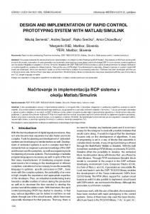
Figure 1.

The residual resampling algorithm.

M a new set of resampled particles {˜x(m) n }m=1 with equal weights 1/M is formed. The basic operations of the RR algorithm are shown in Figure 1. The output r , is an array of replication factors which shows how many times each particle is replicated. We should note that RR is composed of two steps. In the first step, the number of replications of particles is calculated and the particles are stored in memory (blocks 1 and 2). Since this method does not guarantee that the number of resampled particles is M, the weights of the residual particles are computed together with the sum of residual particles, and the number of replicated particles Mr (blocks 3 and 4) is computed. The weights of residual particles represent the portion that is not used in the first step due to truncation. The residual particles have to be resampled again in order to produce the remaining M − Mr particles. This can be done by applying the SR algorithm for the remaining particles. A necessary step before applying SR is to normalize the weights which is shown in block 5. The normalized weights are used as input for the SR procedure. Finally the residual particles are formed and written to the memory.

3. 3.1.

Novel Resampling Mechanisms Single PE Particle Filtering

For physical realization, it is critical to have an efficient mechanism that reduces hardware complexity

50

Hong et al.

and maintains filtering performance. The RR algorithm possesses interesting features for fixed-point implementation. The computation of the replication factor r (m) in block 1 in Figure 1 is performed in hardware without multiplication if the number of particles is of the order of two. However, the second step of the RR algorithm can be significantly simplified. The RR implementation requires M divisions for normalization in block 5 and running an additional resampling algorithm for processing normalized residual particles (block 6). In the following text, an approximate method suitable for fixed-point hardware implementation is proposed. It’s main purpose is to replace the second step of RR. Detailed operation of this algorithm and the corresponding architecture are described in [11]. In this section, we describe the operations of a modified resampling algorithm with tagging as well as a different architecture for this algorithm. Before resampling, the particle weights are computed and normalized in the particle update step. The normalized value of each weight is always non-negative and less than one. These weights are quantized with K + 2 bits where K = log2 M. After the quantization via simple truncation, integer representation of the higher K bits corresponds to the number of times the particle should be replicated. For example, for the case when M = 4, the weight of 0.25 is represented binary as 0.0100. The most significant (excluding first bit) K = 2 bits are 01 which means that this particle will be replicated once. Since the number of replicated particles R obtained by simple truncation is less than M, the residuals are processed using the tagging method. Each particle is tagged based on the last three bits of the K + 2 bit

Figure 2.

Table 1.

Truncation scheme for parallel particle filtering.

Last three bits 000 001 010 011 100 101 110 111

Rounding scheme

Results

Tag status

Truncate Truncate Truncate Truncate Truncate Truncate Truncate Truncate

0 0 0 0 1 1 1 1

none Tag2 Tag2 Tag1 none Tag2 Tag1 Tag1

representation of the weights as shown in Table 1. If the last three bits are 011, 110 or 111, the particles are labeled with tag 1 which means that they have a chance to be replicated once more. Particles whose weights end with 001, 010 or 101 are labeled with Tag 2, and they will be replicated only if the total number of replicated R and Tag 1 particles T is less then M. The algorithm and the organization of the memory in which the replicated particles are written are illustrated in Figure 2. The replication factors are computed and the particles are stored into a particle memory PB from address 0 using increasing addresses. The address counter for replicated particles is named ParticleAddress. Tag 1 particles are stored from address M − 1 using decreasing addresses. The address counter for tag 1 particles is named TaggedAddresses. The memory organization during the resampling process is shown in Figure 2(a). During resampling, it can happen that the total number of tagged and replicated particles is greater than M. This condition is tested by checking

Memory organization for residual resampling that uses tagged particles. PB is abbreviation for particle buffer.


Figure 3.

The operations that are performed by the PEs and by the CU. The data exchanged between the PEs and the CU is also shown.

if ParticleAddress < TaggedAddress. If the condition is not fulfilled, then storing tag 1 particles is stopped in order to prevent overwriting of the replicated particles. The replicated particles can overwrite the tagged particles as shown in Figure 2(b). Tag 2 particles are stored in a dedicated memory (block 8) and they are used only if after resampling T + R < M. In this case, it is necessary to transfer missing particles from the tag 2 memory to the particle memory. This situation is presented in Figure 2(c). 3.2.

Particle Sharing Scheme

A particle filter with 4 PEs is used to speed up the process by parallel operations. In order to support correct operation in multiple PEs configuration, an additional unit, which is the focus of this investigation, called the central unit (CU) is needed. The algorithms for parallel particle filtering called distributed resampling algorithms with proportional allocation (RPA) and non-proportional allocation (RNA) of particles are described in [12]. In this paper, the CU is designed to support both of these algorithms with different modes. Table 2.

51

Each PE performs in parallel the particle update and particle generate steps. Together with the weight computation (particle update), PEi computes the local sum of weights sumi for i = 1, 2, ..., P. Then the PEs send the local sum to the CU and receive the total sum sumtotal . The total sum is used for weight normalization which is done locally within each PE. Then the PEs perform resampling in order to determine the replication factors r (m) for m = 1, ..., M. The CU is mainly responsible for two basic operations (Figure 3). The first operation is done before resampling in which it gathers the sum of the weights generated from each PE and computes the summand (sumtotal ). In the second operation, the CU assists during the exchange of particles after resampling. This process is called state update. We can distinguish between different algorithms and different modes based on how the normalization and particle exchange are performed. Different modes are shown in Table 2. There are a total of 7 different configurations. The coding of each configuration (mode) is also shown in the table. These modes are illustrated in Figure 4.

Illustration of particle sharing modes.

Mode

Configuration

Resampling algorithm

Mode

0 1 2 3 4 5 6

single PE 2-fixed 2-2-fixed 2-2-fixed 2-2-mixed 2-2-adaptive 4-mixed

Resampling algorithm with tagged particles Only 2 PEs are used 2 separate particle filters each using 2 PEs RNA without regrouping RNA with regrouping with defined rules RNA with adaptive regrouping RPA

000 001 010 (2) 011 100 101 111

52

Hong et al.

Figure 4. Illustration of particle sharing for fixed, mixed and adaptive configurations.

The state update requires extensive data communication among the PEs and the CU. In the example shown in Figure 5, a particle filter with P = 4 PEs and M = 16 particles is used. The particles and their weights are computed during the particle generate and particle update steps. In this example, it happened that most of the probability mass is contained in PE2. The normalized sums sumi for the PEs 1 to 4 are: 0, 13/16, 0, 3/16. In this example, the algorithm with proportional allocation is used (RPA), so that each PE generates the number of particles as a result of resampling proportional to its local sum. So, PE1 generates 0 replicated

particles, PE2 13 replicated particles and so on. It was shown in [12] that RPA produces the same resampling result as the sequential resampling algorithms. In order to start the next particle filtering iteration, the number of particles in each PE has to be the same, namely four. So, PE2 has to send its particle surplus to the PEs 1, 3, and 4. The way that it is done in RPA is shown in Figure 6(a). It can be noticed from this example that the communication pattern during the particle exchange is random. Namely, after each particle filtering operation, it is not known which PE will have surplus and which will lack particles. So, the direction and the amount of particles exchanged among the PEs is unknown. We refer to the implementation of the RPA algorithm as 4-mixed configuration. In order to reduce the amount of particles exchanged through the network as well as to make the communication deterministic, the parallel particle filtering algorithm with non-proportional allocation (RNA) is used. The main difference between RNA and RPA is that in RNA the PEs are grouped in groups of two and they act almost as separate particle filters. Let us assume that the sums sumi for the PEs 1 to 4 are: 0, 13/16, 0, 3/16 as in the previous example. Also, let us assume that PE1 and PE2 form one group and PE3 and PE4 form another group as it is shown in 6(b) using solid lines. The resampling is done inside these groups as if they are separate particle filters. Since all the probability mass is contained in PE2, it has to send four particles to PE1. The same happens in the second group, i.e., PE3 sends four particles to PE4. After resampling, the weights of the particles are not equal as in the RPA algorithm. They are set to the sum of the weights of the group. In the first group composed of PE1 and PE2, the sum of the weights is 13/16 so that the weights of the

Figure 5. In this example, a particle filter with 4 PEs and 16 particles is used. The posterior distribution of the unknown is presented. After resampling, the most of the propability mass is contained in PE2.


Figure 6. The example of particle exchange for a) RPA and b) RNA algorithm in which the groups are formed from two PEs.

replicated particles are 13/16. The implementation of the RPA algorithm with fixed groups is referred to as 2-2 fixed (Mode 3) configuration. If the groups are fixed, the weights in one group can become dominant in comparison to the weights from another group. In the case of unequally distributed weights, the particle filter performance will deteriorate because only one half (one group) of particle filter will contribute to the final estimate. This problem is solved by regrouping the PEs. In Figure 6(b), new groups are formed from PE1 and PE3, and PE2 and PE4 shown with dashed lines. Regrouping can be done using some defined rules or adaptively. The rule that is used in Figure 6(b) is that groups are formed alternatively as PE1-PE2, PE3-PE4 and PE1-PE3, PE2-PE4. In adaptive configurations, the groups are formed in a way that the PE with the largest weight is grouped with the PE with the smallest weight. In this way, weights of

53

particles are more evenly distributed among the PEs. The implementation of the RPA algorithm with regrouping with fixed rules is referred to as 2-2 mixed (Mode 4) and with adaptive regrouping as 2-2 adaptive (Mode 5). Several additional modes are considered. For a single PE operation (Mode 0), the resampling is integrated into each PE and no particle sharing scheme is presented. Four independent particle filterings with different parameters can be processed concurrently. Although a single PE mode is supported by the proposed resampling units, a PE with integrated resampling unit is more efficient in terms of data access and speed [13]. In Mode 1, only two PEs are active. In Mode 2, two fixed groups made of two PEs each are formed. There is no interaction among these two groups, and therefore two separate particle filters. 4. 4.1.

VLSI Implementation Single PE Resampling Architecture

We have designed and analyzed two viable resampling schemes. These two schemes illustrated in Figure 7 are suitable for particle filter implementation with a single PE. Its extension to the multiple PE case is described in the next section. The resampling mechanisms start as soon as the first data are read out by the state buffer (SB) and the weight buffer (WB). The data stored in SB consist of four-dimensional vector of the states (x, y, Vx and Vy ) for the case of bearings-only tracking application, and those stored in WB are a one-dimensional

Figure 7. Logic diagram illustrating the structure of the proposed resampling schemes. It is assumed that the particles and their weights are provided before resampling.

54

Hong et al.

vector of the weights. WB stores decimal equivalent representation of the weights which are used to replicate the particles stored in SB. The resampling scheme RS1 is shown in Figure 7(a). In this scheme, particles are copied to a buffer (PB) that stores the fourdimensional vector of the states. The number of copied particles is determined by the relative value of the corresponding weight stored in the WB. After resampling, the resampled particles are copied from PB into another state buffer (SB ) which is the input in the next sampling step (particle generate). For RS1 shown in Figure 7(a), each weight is read out from WB and decoded. An integer value of K bits representing r is loaded to down-counter for particle replication. Depending on the value of r , the downcounter generates a pulse every cycle for r consecutive cycles. The incrementor2 increments the write address of PB if there is a pulse generated from the downcounter. Once the output from the down-counter is 0 (finish counting), the incrementor1 will increment the read addresses of both SB and WB. The read between WB and PB has an offset M + 1 cycles. This offset is chosen to handle the worst case weight distribution in WB where only the weight at the M th address is nonzero and the rest are zero. Additional cycle added to M is the buffer access time of PB. While a particle is being replicated in PB starting from the lowest address, the same particle, if it is tagged (Tag1), is also written to the same memory but starting from the highest address. This is to ensure that the tagged particles can be over-written and discarded. Thus, the total number of replicated particles is always M. However, it is still possible that the sum of R and T is less than M. This possibility is handled by having a small Tag2 memory for storing tagged particles (Tag2) and these particles will be copied to PB only if R + T < M. The inequality is checked by adding the last memory addresses where the replicated particles and tagged particles are inserted. If the sum of these two addresses is less than M, tagged particles (Tag2) will be inserted from (R +1)th address of PB. The Tag2 memory can store at most 128 particles with Tag2. If T2 is more than 128, the tagged particles in Tag2 memory will be over-written. The structure has data feedforward property. Although we have assumed that the number of particles is a power of two, the scheme can be extended to handle an arbitrary number of particles. The difference will be in the tagging method. This resampling structure actually forms a local controller for generating the read addresses of SB and WB.

It is observed that particles are unnecessarily copied twice in this scheme. Copying particles from SB to PB can be avoided by using index addressing. An alternative way to implement the resampling structure, RS2, is shown in Figure 7(b). The four states of one particle have the same address location in SB. So, RS2 adopts a memory (AB) with 1M size to store addresses of these four states instead of using PB with 4M size. Besides, RS2 maintains the same cycle time of resampling as that of RS1. The other operations of RS2 are the same as those of RS1. Let the resampling time be defined as a time between the first access of r and the end of successfully transmitting the last replicated particle to PB or AB. The timing of the single PE particle filtering as well as the resampling time is illustrated in Figure 8. The resampling process begins as soon as the last weight is computed by particle update. The output generate for the current iteration (iteration i) and the particle generate for the next iteration (iteration i + 1) begin at the first access of SB or AB, which is the (M + 1)th cycle after the beginning of resampling. The resampling process and the state update take 2M cycles. The main reason for the 2M cycle latency of output generate is to support the worst case timing of resampling. The worst case occurs when the values of all the weights are zero except the last one. So, the replication of the particles will start at the M th cycle after the beginning of the resampling process. Both RS1 and RS2 are not efficient in the multiple PE operation. Without proper mechanism to support the multiple PE operation, the resampling time cannot be improved even though the number of cycles taken by other unit operations (from particle generation to weight normalization) is reduced by P. Here P is the number of PEs processed in parallel. 4.2.

Multiple PE Resampling Architecture

The proposed architecture that consists of four PEs supports the configuration of different modes shown in Table 2 . It is reconfigurable so that any two PEs can share their particles in any iteration. By properly controlling the connections, any two PEs can share their particles via the CU without conflicts. The timing of the multiple PE resampling is illustrated in Figure 8(b). The processing time of the individual operation is reduced by P. For the worst case timing of resampling, the first particle from PEi is sent to the CU at t . After two additional cycles overhead time due to buffers accesses


55

Figure 8. Illustration of the resampling time. (a) In single PE resampling, t1 is the beginning of the resampling and state update for iteration i. t2 is the beginning of the output generate for iteration i and the particle generate for iteration i + 1. t1 and t2 are separated by at least M + 1 clock cycles. In addition to the M cycles, one additional cycle is added because the particles will be transferred from PB or AB. t3 is the end of resampling and state update, and t4 is the end of output generate. (b) In multiple PE resampling, there are two cycles overhead time due to buffers accesses defined as difference between t1 and t1 .

in the CU, PE j starts to receive particles from the CU at t . The interactions between the PEs and the CU as well as their connections are shown in Figure 9. In maximum, four PEs are processed in parallel. For the best case of resampling, each PE replicates M/P particles. However, some PEs may replicate more than M/P particles and others less than M/P. This is because the sum that each PE uses for weight normalization is sum total and not the sum generated locally from each PE. In other words, the sum of weights for each PE is not balanced. The PEs with particle surplus send the exceeding particles to the CU, and the PEs with missing particles receive particles from the CU. Since the number of particles generated by each PE is proportional to the normalized sum of weights, it can be determined if the PE has exceeding or missing particles. Based on this information, the CU distributes particles. Unlike

in the single PE resampling scheme, tagged particles will not be stored locally. Instead, the tagged particles will be sent to the CU. After the exceeding particles are transferred to other PEs, tagged particles in the CU are used only if there are still some PEs with missing particles. The reason for sending tagged particles to the CU is to exchange particles among different PEs even when the sums of weights are balanced. When the sums of weights are equally balanced among the PEs, all the particles are used only by the corresponding PE. By redistributing the tagged particles, all other PEs will receive surplus form the other PEs as if the processing is done by a single PE. As shown in the figure, a two-level interconnection is adopted. The first level is used for interactions between the PEs and the CU and the second level is exploited for interactions inside the CU. In the figure, RBi and RTBi are buffers used to store exceeding particles which will

56

Hong et al.

Figure 9.

A parallel PE resampling architecture.

be transmitted to different PEs respectively. TBi is a buffer used to store only tagged particles. Particles are written to RBi and TBi in the CU by the resampling interface (RS I/F) of PEi and they are read by the RS I/F of PE j where j = i. Also, particles can be written to RBi from RTB j . It is important to stress that the first level interconnection supports reconfigurability. Connections can be reconfigured in order to support several different modes of operations. The first level interconnection shown in the figure is an example where each PEi gets particles from RBi−1 . In the first level interconnection, not all PEs can exchange particles among themselves. This problem is addressed through the second level of interconnection where unconnected PEs are indirectly connected using RTBi . The second level interconnection is fixed (it is not reconfigurable). RTBi contains two banks, RTBia and RTBib , which are connected to designated RBs respectively. RTBi gets the exceeding particles directly from PEi and the tagged particles from TBi . TBi is accessed after all the particles stored in RBs or RTBs are sent out to the PEs. The sizes of RBi and TBi are chosen to handle the worst case condition for the four-dimensional vector of the states. Among the configuration modes, the worst case happens when 2 PEs process in parallel. Even though it is possible that all the particles generate tags, we chose the size of TBi as (M/2) × 10% × 4(states) = M/5 for 2 PEs mode because usually the tagged particles are around 10% of total replicated particles [11]. Data in RBi are read out after M/2 + 2 cycles of

resampling. But it is possible that before they are read out, all the particles supporting the designated PE of this RBi are generated. The RBi should be large enough to handle this situation. Therefore, the size of each RBi is chosen to be M/2 × 4 = 2M. The overflow buffer is used when the 4-mixed configuration is adopted. Once the data are written in the overflow buffer, they are read out as soon as possible by their designated RBi . However, RTB ja has to stall transferring its particles to RBi until RBi stops receiving particles from PEi . Also, RTBkb has to wait to transfer its particles to RBi until RTB ja has sent all its particles to RBi . The worst case amount of particles that have to be stored in the overflow buffer determines the size of the two banks of overflow buffer. Let us consider the case where four PEs are processed in parallel. There are situations where each PE1 , PE2 , PE3 has large value of R (R > M/P), and PE4 has a small value of R (R < M/P). In this case, many replicated particles from PE1 , PE2 and PE3 will be stored in RTB1b , RTB2a and RB3 , respectively, and then will be used by PE4 . For a situation where PE1 and PE3 have large values of R but PE2 and PE4 have small values of R, most of the particles will be used without having to transfer to overflow buffer. 4.3.

Interface and Control

In order to minimize the resampling time in the multiple PEs operation, resampling has to replicate as many particles as possible in one cycle. For example, if the


Figure 10.

57

R S3 scheme.

replication factor for particle m is r (m) = 4 in only one PE with surplus of particles (Ri > M/P), then this particle should not only be written to the PB but also be sent to the CU in one clock cycle. The CU treats this particle as three which will be buffered in three different memories in the CU. In this case, resampling takes only one clock cycle to copy the particle for r (m) = 4. Without this modification, the resampling time is the same as that of a single PE. The reason is that particle allocation in the CU takes M cycles. With this modification, the resampling time is reduced by a factor of 1/P in average. However, the resampling scheme in the PE has to support the computation of the number of particles that resampling has sent to the CU in one clock cycle, so that the read addresses of both S B and WB are generated correctly. This modified scheme, R S3, is shown in Figure 10, which actually forms the RS I/F in Figure 9. One bit signal sri is generated by comparing sum i and M/P. It indicates whether the PEi has exceeding particles (PEi in sending operation, sri = 0) or missing particles (PEi in receiving operation, sri = 1). For the PEi in sending operation, during the first M/P cycles, the PEi sends particles to the CU. One bit signal ti

informs the CU whether the coming particle is tagged or not. The PEi in receiving operation only sends tagged particles to the CU during the first M/P cycles and will receive particles from the CU after M/P + 2 cycles. The received particles are written to PB starting from the (sumi + 1)th address. Meanwhile its own particles may still be copied from S B to PB depending on the weight distribution in WB. The NSP generator generates a 2-bit signal nspi which indicates how many particles are sent to the CU from PEi in one cycle. nspi will be further used to calculate the number of cycles that R S3 takes to process a weight with r so that the read address of S B and WB is generated correctly. In order to describe the generation of nspi , several control signals are defined. The signal filledi is a one bit signal that indicates whether the highest write address of PB is accessed. The CU calculates the rough number of particles to be transferred to PE j by PEi . When PEi in sending operation generates enough particles for PE j , one bit signal s f i generated in the CU switches from low to high. In the table, there are three signals, s f i , s f ia and s f ib corresponding to the other three PEs. If PEi does not need to support PE j , its corresponding s f signal is always

58

Table 3. nspi

Hong et al.

Conditions for generating nsp. Number of particles sent to the CU in one cycle

01

1 particle

10

2 particles

11

3 particles

00

0 particle

high. A control signal mode contains three bits, m 0 , m 1 and m 2 which are used by the NSP generator instead of s f i , s f ia and s f ib when it is in single PE mode (m 0 = m 1 = m 2 = 0). The maximum number that nspi can represent is 3 since maximum three PEs require particles from PEi . The conditions for generating nspi are listed in Table 3. For example, the CU treats the particle from PEi as three particles (nspi = 11) under the following conditions. First, PEi must not be in a single PE mode. If PEi is in a single PE mode, nspi is always 00, which means that the CU does not accept any particle from PEi . Also, PEi must be in sending operation (sri = 0). Under these constraints, r for the weight must be at least 3. When r = 3, the CU treats this particle as three only if the PB in PEi is filled (filledi = 1) and the CU has not received enough particles from PEi (s f i = s f ia = s f ib = 0). On the other hand, when r > 3, the CU treats this particle as three only if PEi does not generate enough particles for the other three PEs regardless if PB in PEi is filled or not. Once nspi is generated, R S3 starts to calculate the number of cycles which it takes to process a weight with the replication factor r . The factor r is first subtracted by (nspi + 1) if its own PB is not filled, where 1 stands for one particle to fill its own PB in one cycle. If the PB is filled, r is subtracted by nspi . If the subtracted value sub is smaller than or equal to 0, this means, in the next cycle, the same weight and particle will not be read again. The case of sub < 0 occurs when r = 0. Then the gated clock disables the Incrementor2; otherwise it produces a pulse to Incrementor2 controlling the write

Conditions (sri = 0) and (m 0 m 1 m 2 = 000) and { (r=1 and filledi =1) or (r=2 and filledi =0 and at least one of (s f i , s f ia , s f ib ) equals to 0) or (r=2 and filledi =1 and only one of (s f i , s f ia , s f ib ) equals to 0) or (r ≥ 3 and only one of (s f i , s f ia , s f ib ) equals to 0) } (sri =0) and (m 0 m 1 m 2 = 000) and { (r=2 and filledi =1 and at least two of (s f i , s f ia , s f ib ) equals to 0) or (r=3 and filledi =0 and at least two of (s f i , s f ia , s f ib ) equals to 0) or (r=3 and filledi =1 and only two of (s f i , s f ia , s f ib ) equals to 0) or (r ≥ 4 and only two of (s f i , s f ia , s f ib ) equals to 0) } (sri =0) and (m 0 m 1 m 2 = 000) and { (r=3 and filledi =1 and all of (s f i , s f ia , s f ib ) equals to 0) or (r ≥ 4 and all of (s f i , s f ia , s f ib ) equals to 0) } otherwise

addresses of PB so that particles from S B can be written to PB. When sub ≤ 0, in the next cycle, Incrementor1 will be incremented and the next weight and particle will be read out correctly. The logic of R S3 computes the number of particles sent to the CU in one cycle. However, it has no information which PE will receive these particles. This assessment is made by the CU.

5. 5.1.

Architecture Evaluation Inter-Chip Data Communication Analysis

Figures 11 and 12 illustrate the number of particle communications between PEi and the CU in term of M for 2-fixed, 2-2-fixed, 2-2-mixed and 4-mixed modes. Both R S1 and R S3 schemes are compared. Assume that the sum of all the local R of each PE is M. Tagged particles are not considered here. Since the power consumption is especially expensive for inter-chip data communication, it is highly desirable to minimize the particle communications between the PEs and the CU. Figure 11 shows the case for 2-fixed and 4-mixed modes. For 2-fixed mode, when R = 0.5M in each PE, the sums of the weights in the two PEs are equally balanced and no particle needs to be transferred between PEi and the CU. PEi is in sending operation when R > 0.5M and in receiving operation when R < 0.5M. The advantage of using R S3 in each PE cannot be shown in this mode in term of data communication and it has the same performance as that of R S1.


59

Figure 11. Relationship between the value of R of PEi and the number of particle communications between PEi and the CU for the 2-fixed and 4-mixed modes. y-axis represents the normalized (by M) number of data transfers.

This is because in this mode each cycle the CU receives only one particle from PEi in maximum when PEi is in sending operation. When PEi is in receiving operation, the particles are received sequentially by both the R S1 and RS3 schemes. For a 4-mixed mode, the sum of the weights in the four PEs are balanced when R = 0.25M in each PE. PEi sends particles to the CU if R > 0.25M and receives particles from the CU if R < 0.25M. For the use of R S1, the number of data communications is proportional to the number of exceeding or missing particles of PEi . This is also true for R S3 when PEi is in receiving operation due to the sequential nature of the receiving particles. When PEi is in sending operation, the CU can receive at most three particles from R S3

in one cycle for the best situation and the number of communicated data is reduced. Otherwise the CU may also receive particles sequentially for R S3 depending on the weight distribution in PEi . Figure 12 illustrates the number of particle communications between PEi and the CU for the 2-2-fixed and 2-2-mixed modes. For the same reason as for the 2-fixed mode, it makes no difference of using R S1 and R S3 for both modes. The sums of the weights in the four PEs are balanced when when R = 0.25M in each PE. PEi sends particles to the CU if R > 0.25M and receives particles from the CU if R < 0.25M. For both modes, for the best case where the number of particle communications is minimum, PEi cannot send all its exceeding particles or receive all the missing particles. For PEi

Figure 12. Relationship between the value of R of PEi and the number of particle communications between PEi and the CU for the 2-2-fixed and 2-2-mixed modes. y-axis represents the normalized (by M) number of data transfers.

60

Hong et al.

in receiving operation, this number is reduced to 0. This is because PEi and its designated PE, PE j , are both in sending or receiving operation. On the other hand, the worst case happens when PEi has to transmit or receive a full amount of particles to/from PE j . For R = M in PEi for both modes, the other three PEs must be in receiving mode. In this situation, PEi has 3M/4 exceeding particles but it only needs to transmit M/4 particles to PE j . In the 2-2-mixed mode, for R = M/2 and R = 3M/4, the number of particle communications for the best case is different from 0 since the PE with largest value of R has to share its particles with the PE with smallest value of R. When the particles are evenly distributed in the other three PEs, the number of particle communications is minimized.

5.2.

Chip Implementation

The CU chip has been designed and implemented using Cadence with TSMC 0.35μm, 4 metal CMOS process. The layout is shown in Figure 13. The CU chip contains 360 pins surrounding evenly on the four sides. The total number of pins depends on the dimensionality of the dynamic system. The particle filter considered in this

paper has a dimensionality of 4. The overall CU chip size is 9.5 mm × 9.6 mm. The major area is dominated by the memory and interconnect. The first level interconnection which supports reconfigurability is located between the pins and the R Bs. Each of the interconnect line contains transmission gate switch for multiplexing to select correct routing paths. As we have discussed, this first level interconnect supports non-deterministic nature of data transfers between the processing elements. Each R B is facing each side of the chip in order to minimize interconnect paths to the PEs. The overflow buffers and a central controller are located in the center of the chip. The central controller is responsible for generating all the control signals of the CU. It also includes logic for generating the sumtotal . The speed of the CU is limited by the largest dual-port static memory whose size is 4k × 16 bits with four banks. Each memory cell is designed with 6-T SRAM cell configuration. The maximum achieved clock speed of the CU is 284 MHz. The capacity of the particle filters (i.e., the value of M) can be increased by incorporating larger memory in the unit. An efficient placement of the memory and interconnect is one of the advantages over the FPGA realizations in terms of area and speed. 5.3.

Figure 13. The layout of the CU (9.5mm × 9.6mm). The CU is designed and implemented using Cadence with tsmc 0.35μm, 4 metal CMOS process.

Performance Comparison

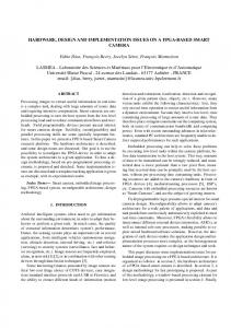
We compare the performance of the CU unit with that of commercial DSP (TI TMS320C67xx series). Fig. 14 illustrates the execution time of the resampling units only. Fig. 14(b) shows curves without DSP. The execution time is plotted as a function of the particles, M. In determining the execution time of the DSP, the VLSI implementation is replaced by the DSP with standard memory address scheme. A standard bus structure with the External Memory Interface (IMIF) of the DSP is modeled for multiple PEs configuration [14]. The DSP is running at 600 MHz. The execution time of the DSP is determined with TI Code Composer instruction profiling tool. The bus performance is modeled with the Verilog for computing data exchange time. Three plots for multiple PE execution time is plotted for the VLSI implementation. Note that increase in the number of PEs does not significantly increase the performance. However, multiple PEs reduce overall particle filtering by a factor of P where P is the number of PEs. Thus, overall execution time for multiple PEs will be significantly faster. On the other hand, the performance is significantly degraded due to


6.

61

Conclusion

In parallel particle filters, resampling is the most critical unit that directly influences the performance and overall hardware complexity. In this paper, we have proposed and designed a flexible resampling architecture that can be employed for high throughput particle filtering. A very efficient resampling mechanism is incorporated which reduces the overall resampling time by a factor of the number of PEs. The unit is synthesized using 0.35 μm CMOS processing technology and its performance is evaluated. The design supports up to four parallel PEs executing bearings-only tracking application with various modes of operations. The number of PEs is limited only by the number of input/output pins. The architecture presented in this paper can be extended to other particle filters.

References

Figure 14. Performance comparison. DSP is running at 600 MHz with standard address scheme and the bus structure. (a) Curves with DSP. (b) Curves without DSP.

extensive sequential memory access. Even though the clock speed of the DSP is higher than that of the VLSI implementation, the overall resampling time does not change for multiple PEs. There is a slight but insignificant increase in the execution time due to overhead in handshaking mechanism (i.e., the I/O pins of the DSP is time-multiplexed where the data transfer becomes serialized). In both platforms, the capacity of the particle filter can be increased since the memory requirement is linear in M. In the VLSI implementation, more memory needs to be incorporated to support higher capacity without any change in the interconnect topology. On the other hand, the DSP requires a large amount of external memory, which significantly affects the performance of the overall operation.

1. A. Doucet, N. de Freitas, and N. Gordon, Eds., Sequential Monte Carlo Methods in Practice, New York: Springer Verlag, 2001. 2. M. Bolić, P. M. Djurić, S. Hong, “New Resampling Algorithms for Particle Filters,” IEEE ICASP, 2003. 3. M. Bolić, P. M. Djurić, S. Hong, “Resampling Algorithms for Particle Filters: A Computational Complexity Perspective,” submitted to the Journal of Applied Signal Processing, 2003. 4. M. Bolić, P. M. Djurić, S. Hong, “Resampling Algorithms for Particle Filters Suitable for Parallel VLSI Implementation,” IEEE CISS, 2003. 5. R. Tessier and W. Burleson, “Reconfigurable Computing and Digital Signal Processing: A Survey,” Journal of VLSI Signal Processing, May/June 2001. 6. Xilinx, “Virtex-II Platform FPGA Handbook,” 2000. 7. N. J. Gordon, D. J. Salmond, and A. F. M. Smith, “A novel approach to nonlinear and non-Gaussian Bayesian state estimation,” IEE Proceedings F, vol. 140, pp. 107–113, 1993. 8. E. R. Beadle and P. M. Djurić, “A fast weighted Bayesian bootstrap filter for nonlinear model state estimation,” IEEE Transactions on Aerospace and Electronic Systems, vol. 33, pp. 338–343, 1997. 9. D. Crisan, P. Del Moral, and T. J. Lyons, “Non-linear filtering using branching and interacting particle systems,” Markov processes and Related Fields, vol. 5, no. 3, pp. 293–319, 1999. 10. J. S. Liu, R. Chen, and W. H. Wong, “Rejection control and sequential importance sampling,” Journal of American Statistical Association, vol 93, no.443, pp. 1022–1031, 1998. 11. S. Hong, M. Bolić, and P. M. Djurić, “An Efficient Fixed-Point Implementation of Residual Systematic Resampling Scheme for High-Speed Particle Filters,” IEEE Signal Processing Letters, vol. 11, No. 5, May 2004.

62

Hong et al.

12. M. Bolić, P. M. Djurić, S. Hong, “Resampling Algorithms and Architectures for Distributed Particle Filters,” accepted for publication in IEEE Transactions on Signal Processing, 2004. 13. S.-S. Chin and S. Hong, “VLSI Design and Implementation of High-Throughput Processing Elements for Parallel Particle Filters,” IEEE SCS, 2003. 14. FPGA Interface to the TMSC6000 DSP Platform Using EMIF, Xilinx Inc. - XAPP753, May 2004.

Miodrag Bolić received the B.S. and M.S. degrees in electrical engineering from the University of Belgrade, Yugoslavia, in 1996 and 2001, respectively, and his Ph.D. degree in electrical engineering from Stony Brook University, NY, USA. He is currently with the School of Information Technology and Engineering at the University of Ottawa, Canada. From 1996 to 2000 he was Research Associate with the Institute of Nuclear Science Vinˆca, Yugoslavia. From 2001 to 2004 he worked parttime at Symbol Technologies Inc., NY, USA. His research is related to VLSI architectures for digital signal processing and signal processing in wireless communications and tracking. Sangjin Hong received the B.S and M.S degrees in EECS from the University of California, Berkeley. He received his Ph.D in EECS from the University of Michigan, Ann Arbor. He is currently with the department of Electrical and Computer Engineering at State University of New York, Stony Brook. Before joining SUNY, he has worked at Ford Aerospace Corp. Computer Systems Division as a systems engineer. He also worked at Samsung Electronics in Korea as a technical consultant. His current research interests are in the areas of low power VLSI design of multimedia wireless communications and digital signal processing systems, reconfigurable SoC design and optimization, VLSI signal processing, and low-complexity digital circuits. Prof. Hong served on numerous Technical Program Committees for IEEE conferences. Prof. Hong is a Senior Member of IEEE.

Shu-Shin Chin was born in Kaohsiung, Taiwan, ROC, in 1974. He received his M.S. and Ph.D degrees in electrical and computer engineering from Stony Brook University – State University of New York in 1999 and 2004, respectively. His research interests include low-power digital circuits, and coarsegrained reconfigurable architectures for high-performance DSP systems.

Petar M. Djurić received his B.S. and M.S. degrees in electrical engineering from the University of Belgrade, in 1981 and 1986, respectively, and his Ph.D. degree in electrical engineering from the University of Rhode Island, in 1990. From 1981 to 1986 he was Research Associate with the Institute of Nuclear Sciences, Vinˆca, Belgrade. Since 1990 he has been with Stony Brook University, where he is Professor in the Department of Electrical and Computer Engineering. He works in the area of statistical signal processing, and his primary interests are in the theory of modeling, detection, estimation, and time series analysis and its application to a wide variety of disciplines including wireless communications and bio-medicine. Prof. Djurić has served on numerous Technical Committees for the IEEE and SPIE and has been invited to lecture at universities in the US and overseas. He is the Area Editor of Special Issues of the Signal Processing Magazine, the Treasurer of the IEEE Signal Processing Conference Board, and Associate Editor of the IEEE Transactions on Signal Processing. He is also the Chair elect of the IEEE Signal Processing Society Committee on Signal Processing—Theory and Methods, and an Editorial Board member of Digital Signal Processing, the EURASIP Journal on Applied Signal Processing and the EURASIP Journal on Wireless Communications and Networking. Prof. Djurić is a Member of the American Statistical Association and the International Society for Bayesian Analysis.