Design and Implementation of Parallel Algorithms ... - Semantic Scholar

Design and Implementation of Parallel Algorithms for Modern Heterogeneous Platforms Based on the Functional Performance Model

David Clarke UCD student number: 09155660

The thesis is submitted to University College Dublin in fulfilment of the requirements for the degree of

Doctor of Philosophy in Computer Science

School of Computer Science and Informatics Head of School: John Dunnion

Research Supervisor: Alexey Lastovetsky

April 2014

Contents

Contents

i

Abstract

v

Acknowledgements

viii

1 Introduction

1

1.1 Contributions of this Research . . . . . . . . . . . . . . . . . .

5

1.1.1 Criticism of Traditional Data Partitioning Algorithms Based on Constant Performance Models

. . . . . . . .

6

1.1.2 New Algorithm Based on Functional Performance Models and Numerical Solution of Data Partitioning Problem

6

1.1.3 Dynamic Data Partitioning Algorithm and Partially Built Functional Performance Models . . . . . . . . . . . . .

7

1.1.4 1.5D Matrix Partitioning Algorithm . . . . . . . . . . . .

8

1.1.5 Hierarchical Data Partitioning Algorithm . . . . . . . . .

9

1.1.6 Benchmarking and Using Performance Analysis Tools for Construction of Function Performance Models . . . .

9

1.1.7 FuPerMod: a Software Framework for Data Partitioning .

11

2 Background

12

i

2.1 Heterogeneous HPC Platforms . . . . . . . . . . . . . . . . . .

12

2.2 Scheduling, Data Partitioning and Load Balancing . . . . . . .

15

2.2.1 Task Scheduling . . . . . . . . . . . . . . . . . . . . . .

17

2.2.2 Data Partitioning . . . . . . . . . . . . . . . . . . . . . .

18

2.2.3 Heterogeneous Data Partitioning Problem . . . . . . . .

21

2.3 Data Partitioning Based on the Constant Performance Model

.

23

2.3.1 Criticism of Traditional Data Partitioning Algorithms Based on Constant Performance Models

. . . . . . . .

27

2.4 Software Frameworks for Data Partitioning and Load Balancing

35

3 Building Models

36

3.1 Modelling the Computational Performance of Heterogeneous Processors . . . . . . . . . . . . . . . . . . . . . . . . . . . . .

36

3.1.1 Computational Unit . . . . . . . . . . . . . . . . . . . .

36

3.1.2 Complexity of Computations . . . . . . . . . . . . . . .

37

3.1.3 Performance Measurement Point . . . . . . . . . . . . .

37

3.1.4 Benchmarking with a Computational Kernel . . . . . . .

38

3.1.5 Benchmarking with instrumented tracefiles

. . . . . . .

40

3.2 Fitting Continuous Curves to Models . . . . . . . . . . . . . . .

41

3.2.1 Piecewise Linear Approximations . . . . . . . . . . . . .

42

3.2.2 Akima Spline Interpolation . . . . . . . . . . . . . . . .

43

3.3 Construction of Partial Speed Functions . . . . . . . . . . . . .

44

3.3.1 Construction of Partial Piecewise Linear Approximations

45

3.3.2 Construction of Partial Akima Spline Interpolation . . . .

46

3.4 Two-dimensional Functional Performance Models . . . . . . . .

46

4 Partitioning Based on the Functional Performance Model 4.1 Geometric Partitioning Algorithm . . . . . . . . . . . . . . . . .

48 49

ii

4.2 Numerical Partitioning Algorithm . . . . . . . . . . . . . . . . .

52

4.2.1 Convergence and complexity analysis . . . . . . . . . .

53

4.3 Dynamic Partitioning Algorithm . . . . . . . . . . . . . . . . . .

54

4.3.1 Experimental Results . . . . . . . . . . . . . . . . . . .

58

5 Applications

63

5.1 1.5D Matrix Partitioning Algorithm . . . . . . . . . . . . . . . .

63

5.1.1 Column-Based Matrix Partitioning . . . . . . . . . . . .

66

5.1.2 Column Based Partitioning with Communication Minimising Algorithm . . . . . . . . . . . . . . . . . . . . .

66

5.1.3 2D-FPM-based Matrix Partitioning . . . . . . . . . . . .

67

5.1.4 1.5D Matrix Partitioning Algorithm . . . . . . . . . . . .

69

5.1.5 Experimental results . . . . . . . . . . . . . . . . . . . .

71

5.2 Hierarchical Matrix Partitioning . . . . . . . . . . . . . . . . . .

74

5.2.1 Inter-Node Partitioning Algorithm . . . . . . . . . . . . .

76

5.2.2 Inter-Device Partitioning Algorithm . . . . . . . . . . . .

77

5.2.3 Experimental Results . . . . . . . . . . . . . . . . . . .

78

6 Conclusion

83

Bibliography

86

Appendices

99

A FuPerMod: a Software Framework for Data Partitioning

99

A.1 Process Configuration . . . . . . . . . . . . . . . . . . . . . . . 101 A.2 Measurement of Computational Performance . . . . . . . . . . 102 A.3 Models of Computational Performance . . . . . . . . . . . . . . 106 A.4 Static Data Partitioning . . . . . . . . . . . . . . . . . . . . . . 108 A.5 Dynamic Data Partitioning and Load Balancing . . . . . . . . . 110 iii

B List of abbreviations

113

iv

Abstract The importance of heterogeneity in high performance computing is increasing with the advent of specialised accelerators and non-uniform memory access. Most of the top supercomputers in the world are heterogeneous in some form and they are expected to become more heterogeneous in the future with the introduction of many-core processors and energy efficient system-on-chip platforms. To achieve maximum performance on such platforms, parallel scientific applications must adapt to this heterogeneity. Data parallel applications can be load balanced by applying data partitioning with respect to the performance of the platform’s individual devices. However, finding the optimal partitioning is not trivial. Traditional load balancing algorithms parametrise processor performance with a single positive number. This thesis shows that load balancing algorithms based on this approach may fail. We present in this thesis the functional performance model (FPM) as a more accurate description of application performance. The FPM represents device speed as a continuous function of problem size and is application and hardware specific. It includes all contributions from clock cycles, memory operations and hierarchy, and operating system overhead. We have developed data partitioning algorithms which take FPMs as input and produce the optimal load balanced partition. We present a dynamic FPM-based partitioning algorithm, designed for use in situations where each run of the application has

v

unique performance characteristics. It does not require a priori performance models as input. Instead, it produces an approximation of the necessary parts of the speed functions. Some applications require more than one partitioning parameter for efficient parallel execution, for example two-dimensional matrix partitioning for matrix-matrix multiplication on a heterogeneous platform. Partitioning algorithms based on 2D-FPMs can solve this problem, however they bring added complexity. We present a novel matrix partitioning algorithm that produces the balanced partition of matrix in two dimensions by using 1D-FPMs and a communication minimising algorithm. Modern heterogeneous HPC platforms are hierarchical and therefore can be used efficiently only if the hierarchy is taken into account while computations are distributed between computing devices. Heterogeneous HPC platforms have hierarchy in their parallelism. We present a hierarchical data partitioning algorithm which is based on FPMs built dynamically at runtime for different levels of the hierarchy. Through this method we are able to achieve load balancing with a coherent communication pattern while minimising the volume of communication. We prove the effectiveness of this algorithm by applying it to a large-scale parallel matrix multiplication application on a heterogeneous cluster with heterogeneous CPU+GPU nodes. The models, algorithms and applications presented in this thesis are available in FuPerMod, an open-source tool for data partitioning, developed by the author.

vi

Statement of Original Authorship I hereby certify that the submitted work is my own work, was completed while registered as a candidate for the degree stated on the Title Page, and I have not obtained a degree elsewhere on the basis of the research presented in this submitted work.

vii

Acknowledgements First and foremost I want to thank my supervisor, Dr. Alexey Lastovetsky: for being the ideal mentor over the past four years; for your guidance that kept me on the right path; and for interesting discussions on topics from HPC to computer science and beyond. I always came away from our meetings with renewed enthusiasm for the project. You helped me see the bigger picture whenever I lost sight of it. I am eternally grateful for the opportunities you have given me, from trusting in me and inviting me to join your lab in the first place, to the lecturing position, to opening the door for my future career. To my colleague Dr. Vladimir Rychkov, thank you for the details; for the thousand small things that made this project work. From showing me how to write my first parallel programme four years ago, to lessons in software engineering, to writing four handed. You are a good friend, full of never ending thoughtfulness. I have enjoyed our lively debates, about the project, the true nature of a kernel and a data point, and about life in general. This work wouldn’t be at the standard it is without your help. To all my colleagues from the Heterogeneous Computing Laboratory, Kiril Dichev, Ashley DeFlumere, Zhong Ziming, Ken O’Brien, Khalid Hasanov, Tania Malik, Oleg Girko, Amani Al Onazi, Jean-Noel Quintin, Jun Zhu, Brett Becker, Ravi Reddy, Robert Higgins and Thomas Brady; you have been a source of friendship, academic collaboration, and good advice. From the School of Computer Science and Informatics, thank you to John Dunnion, head of school, both for his academic support and for giving me the opportunity of a lecturing position. Thank you also to the school’s support staff: Patricia Geoghegan, Clare Comerford, Gerry Dunnion, Paul Martin, Tony O’Gara and Alexander Ufimtsev for their consistent helpfulness over the years. Thank you Aleksandar Ili´c, Leonel Sousa and Svetislav Momcilovic from INESC-ID, Lisbon, Portugal, for the collaboration, the broadening of horizons,

viii

the lunches, and the solid piece of work we produced together. A special thanks to Aleksandar and Jelena for being such welcoming hosts and tour guides. I would like to thank Dr Emmanuel Jeannot and everyone involved in the ComplexHPC COST Action for the many interesting meetings and workshops hosted around Europe. It was a great opportunity to meet other European researchers working on similar topics to me. I would especially like to thank Emmanuel for sponsoring my user account on the Grid5000 experimental testbed where the majority of the experiments presented in this thesis were performed. Thank you to Maya G. Neytcheva and Petia Boyanova from Uppsala University, Sweden for hosting me on my short term science mission with them. Thank you to all my amazing friends who have supported me throughout, especially to Katie for her help proof reading this thesis. This thesis has emanated from research conducted with the financial support of Science Foundation Ireland under Grant Number 08/IN.1/I2054. Experiments were carried out on Grid’5000 developed under the INRIA ALADDIN development action with support from CNRS, RENATER and several Universities as well as other funding bodies (see https://www.grid5000.fr). This work was also supported by COST Action IC0805 "Open European Network for High Performance Computing on Complex Environments". We are grateful to Arnaud Legrand who provided sample code for minimising the total volume of communication. Thank you to the Barber family, Sue, Iain, Nathan and James for welcoming me into their home, especially to Sue for all of the hot dinners (even if they were often cold when I made it home to them). To my own family Brid, Pat, Nuala, Lorna and Markus I am grateful for the support, encouragement and love throughout my whole life. Finally to my wonderful wife Sian, my love, the shining star that guides my night and brightens my day. You have been there for me every step of the way, and your love makes it all worthwhile.

ix

To my wife and best friend.

x

Chapter 1 Introduction The main goal of high performance computing (HPC) is to increase the efficiency with which scientific applications are executed on dedicated computing platforms. With greater efficiency the total run-time of the application is reduced, larger problems can be tackled and the total energy consumed may also be reduced. HPC platforms are composed of many computational devices working in parallel. In the past, designers of HPC hardware went to considerable effort to make these platforms as homogeneous as possible. Now there is an industry-wide change towards heterogeneous systems, with many of the top supercomputers in the world being heterogeneous by design. This transition is the most significant change since the move from single to multi-core systems. The number of cores has very recently increased by an order of magnitude with massively multicore co-processors being used in the top systems, and soon it will be the norm for there to be hundreds of cores per compute node on most HPC platforms. With many cores it is impossible to provide equal access to memory, which results in non-uniform memory access (NUMA). Furthermore, as the number of cores increases, it is not beneficial for all these cores to be identical. A better approach is to have different cores specialised for different tasks, for example a node with both CPUs and GPU accelerators. In future systems these will be combined on a single chip. Heterogeneity in HPC can also arise from: hardware replacement and

1

upgrade, complex network topology, software heterogeneity, and application specific load imbalance. These current and future heterogeneous platforms present significant challenges to computer scientists. To achieve optimum performance, HPC applications must adapt to the heterogeneity of these platforms. In this thesis we present algorithms for optimising parallel scientific applications on heterogeneous platforms. The majority of parallel scientific applications can be described as iterative, and can be generalised as follows: within each iteration some calculations take place in parallel, then some synchronisation takes place. The subclass of these applications we target are characterised by divisible computation workload, which can be broken into a large number of equal independent computational units. Each processing device on the parallel platform is responsible for the computations associated with these units. Additionally, computational workload is proportional to the size of data and dependent on data locality. Our target architecture is a dedicated heterogeneous distributed-memory HPC platform. We do not confine ourselves to one specific piece of hardware, but instead develop general algorithms which are equally applicable to to a range of hardware from a single CPU/GPU compute node to grid environments, incorporating many heterogeneous clusters. And since the algorithms are general they will also be applicable to future yet to be released many-core platforms. High performance of applications on these platforms can be achieved when all processing devices complete their work within the same time. This is achieved by partitioning the computational workload and the associated data unevenly across all devices. Workload should be distributed with respect to the devices speed, memory hierarchy and communication network, however this unconstrained problem is NP-complete [1, 2, 3]. In the literature many data partitioning algorithms perform load balancing by distributing workload in proportion to device speed. How they compute this speed varies. Some use processor clock speed while others perform synthetic benchmarks, or measure the time to execute all or part of the application. What they all have in common is that they model the speed of each device with a 2

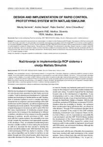
single positive number. We refer to this as the Constant Performance Model (CPM), and refer to the algorithms as CPM-based partitioning algorithms. For medium sized problems executed on general purpose CPUs, CPMbased partitioning algorithms are able to converge to a balanced workload. However, in general, speed is not constant, but instead is a function of problem size (Fig. 1.1). We will demonstrate for a number of applications that, for the full range of problem sizes that can be executed, CPMs are too simplistic and in some situations partitioning algorithms based on them may completely fail to converge. We present the Functional Performance Model (FPM) to be a more realistic model of processor performance than CPM. Under this model, the speed of each processor is represented by a continuous function of the problem size. The shape of each function is found empirically by benchmarking the application as it is executed on the real hardware. FPMs are application- and platformspecific and integrate many important performance features such as memory hierarchy, cache misses, swapping and application specific characteristics. Data partitioning algorithms based on accurate FPMs are able to achieve better load balancing than the more simplistic CPM-based data partitioning algorithms. We present two classes of FPM-based partition algorithms, static partitioners, which take a model for each processing unit as input, and dynamic partitioners, which dynamically generate the necessary models at runtime. The output of both partitioning classes is a vector of distributions which optimally balances the computational workload. In its simplest form, the problem to be solved by the partitioner can be stated as follows.

Given p processing devices with speed functions

s(d1 ), . . . , s(dp ), how can D computational units be distributed such that all processors complete their work within the same time? We present two main FPM-based partitioning algorithms for solving this problem, namely the Geometric Partitioning Algorithm and the Numerical Partitioning Algorithm. The Geometric Partitioning Algorithm is based on the observation that a line, which passes through the origin, marks out a balanced distribution at the points where it intersects the speed functions. The problem is thus reduced to finding the slope of the line which produces the desired total workload, d1 + 3

500 450 400

Speed (GFLOPS)

350 300 250 200 150 100 50 0 0

1e+08

2e+08 3e+08 Matrix elements updated

4e+08

5e+08

Speed (GFLOPS)

(a) 1000 900 800 700 600 500 400 300 200 100 0 0

0.2

0.4

0.6

0.8

1

1.2

1.4

1.6

1.8

Matrix elements (× 109)

(b) 140

adonis 7CPU + 1GPU adonis 1CPU + 1GPU adonis 0CPU + 1GPU

Speed (GFLOPS)

120 100 80 60 40 20 0 0

10000

20000 30000 40000 50000 60000 Problem Size wi (b × b blocks updated)

70000

(c)

Figure 1.1: Functional performance models. (a) Matrix update kernel from a selection of the 75 nodes from Grid’5000 Grenoble. (b) Out-of-core matrix multiplication on NVIDIA GeForce GTX680 GPU. (c) Matrix block update on a hybrid node with multi-core and NVIDIA Tesla T10.

4

1.1. CONTRIBUTIONS OF THIS RESEARCH

d2 + . . . + dp = D. This is achieved by joining the discrete data points with piecewise linear approximations and iteratively bisecting the solution space in order to converge to the solution. Convergence of this algorithm is guaranteed provided there are some minor restrictions placed on the shape of each FPM. Namely for some point x, the function is monotonically increasing and concave in the interval [0, x] and monotonically decreasing in the interval [X, ∞]. FPMs not fitting this profile need to be modified before use with the GPA.

1.1

Contributions of this Research

The main contributions to knowledge that this doctoral research study produced are as follows: 1. Demonstration that, in some situations, existing state of the art CPMbased partitioning algorithms can fail. 2. Proposal of the Numerical Partitioning Algorithm. 3. Development of the Dynamic Partitioning Algorithm and partial FPMs. 4. Proposal of the 1.5D Matrix Partitioning Algorithm. 5. Hierarchical Data Partitioning Algorithm. 6. Building independent FPMs for parallel applications

• from an equivalent serial computational kernel • from instrumented tracefiles. 7. Development of the software framework FuPerMod. In the following sections we introduce each of these contributions.

5


1.1.1

Criticism of Traditional Data Partitioning Algorithms Based on Constant Performance Models

We implemented a dynamic load balancing algorithm, typical of the state of the art, that are aimed at our target application and platform. This algorithm uses CPM-based partitioning and is designed for iterative applications, so we chose to apply it to Jacobi method. When the application was executed with medium sized problems, we achieved the same convergence towards a balanced partitioning as the authors did. However, the load balancing algorithm fails to converge to a balanced result, when we ran the application with a problem size that when partitioned, results in a memory requirement which is close to a memory hierarchy boundary of at least one device. Furthermore, it can enter a cycle of oscillation resulting in large amounts of data transfer with each redistribution. We applied our FPM-based partitioning algorithm to the same problem and it successfully converged to a balanced load [4].

1.1.2

New Algorithm Based on Functional Performance Models and Numerical Solution of Data Partitioning Problem

The GPA applies restrictions on the shape of the FPMs. The piecewise linear approximations used by the GPA must be modified to fit within these restrictions. Often this modification is not a problem since the restrictions describe the general shape of most FPMs. However, for some FPMs the modification can result in reduced accuracy in the final result. A FPM is composed of a series of empirically found data points. A smooth continuous function with continuous derivatives of arbitrary shape can be fitted to these discrete points using Akima splines interpolation. We propose the Numerical Partitioning Algorithm (NPA) as alternative to the GPA [5, 6]. The NPA uses these smooth mathematical curves and expresses the load balancing problem as a system of nonlinear equations (1.1). These equations form a multidimensional root finding problem and can be solved for F (x) = 0 using Powell’s Hybrid method. Where F (x) is given as 6


F (x) =

 p X   D − xi

(1.1)

i=1

 x x1   i − si (xi ) s1 (x1 )

2≤i≤p

The NPA takes one FPM per device and a total problem size as input. It outputs a vector describing the partitioned workload to be assigned to each device.

1.1.3

Dynamic Data Partitioning Algorithm and Partially Built Functional Performance Models

If an application is to be run many times on a stable set of hardware a significant speed-up can be achieved up by building detailed models. However, if each run of the application is considered unique, for example in a grid or cloud environment, when different resources are allocated with each job request, or when changing an application parameter necessitates rebuilding the models, it becomes no longer practical to build full-FPMs as more time may be spent benchmarking than the total runtime of the application. We present the Dynamic Partitioning Algorithm (DPA) as a solution to this problem. The DPA uses partial FPM to find a balanced distribution of workload [7]. With the partial FPMs, only the necessary parts of the speed functions are built, to sufficient detail, to allow the dynamic partitioner to find a balanced load. This load balancing may be performed within the first few iterations of an application, or alternatively immediately before runtime. With a well designed kernel to benchmark, the time spent building the partial models may account for just a small fraction of the total runtime of the application. The idea of building partial FPMs was proposed before the commencement of this doctoral research study. However, this research study has developed and expanded this idea to the state as it is presented here.

7


1.1.4

1.5D Matrix Partitioning Algorithm

For many parallel applications the volume of communication is proportional to the size of the boundary of the partitioned data. For example, in some simulation applications, the volume of communication is proportional to the surface area of the domain decomposition and with matrix multiplication the total volume of communication is directly proportional to the sum of the halfperimeters of the partitioned submatrices. It is better to partition a matrix into a number of rectangles which are close to square rather than long horizontal or vertical slices. This two dimensional partitioning requires two parameters per device to describe it. Neither the GPA nor the NPA, in their standard form, are able to produce such a partitioning. This problem can be solved by building 2D-FPMs and using our 2D-FPM partitioning algorithm [8]. 2D-FPMs are built by benchmarking the application over a range of points (m, n), 0 < m ≤ M, 0 < n ≤ N . This produces a surface in 3D space. Unfortunately, 2D-FPMs require the square of the number of benchmarked points in a 1D FPM in order to achieve the same accuracy. Furthermore, an application may have N degrees of freedom in its partitioning scheme, and thus requiring N -dimensional-FPMs and an N dimensional partitioning algorithm. We have come up with a novel solution to this problem which can produce a two dimensional partitioning from 1D FPMs and we call it the 1.5D Matrix Partitioning Algorithm [9]. To partition a matrix into rectangles, we combine the parameters height and width into a single parameter area. This area represents the volume of computations that a device must perform in each iteration of the application. We benchmark a computational kernel for a range of areas with square shape. This produces a model with speed as a function of area. Either the GPA or NPA can now be used to produce a distribution vector representing the volume of computation to be assigned to each processor. Then a Communication Minimising Algorithm (CMA) is used to arrange the rectangles so that they: (i) exactly tile the matrix, (ii) each have the required area and (iii) minimise the sum of the half-perimeters. A CMA is an application specific algorithm, which arranges the partitioning to minimise communication while

8


maintaining the same workload distribution. We demonstrate how this approach can be successfully applied to matrix multiplication. The same scheme can be extended to applications which employ a partitioning in 3D space, for example computational fluid dynamics, by using one of the many domain decomposition algorithms as the CMA.

1.1.5

Hierarchical Data Partitioning Algorithm

All modern HPC platforms employ hierarchy in their parallelism, ranging from instruction level parallelism to multi-core, multi-socket and multiple accelerators, all the way up to many nodes in a cluster and grids of clusters. To optimise performance data parallel applications can employ a data partitioning scheme which matches this hierarchy. We present the Hierarchical Partitioning Algorithm [10, 11] for load balancing applications running on heterogeneous hierarchical HPC platforms. Applications utilising this algorithm become self-adaptive to the heterogeneity of the platform by dynamically building the performance models at run-time. The algorithm is iterative and alternately partitions a matrix in two dimensions between heterogeneous compute nodes and sub-partitions each of these sub-matrices between the heterogeneous devices within each node. To do this, this algorithm draws on the contributions described in the preceding sections. The application achieves a performance gain from nested parallelism and efficient communication patterns. We present it for use with two levels of hierarchy applied to matrix multiplication, however this scheme can easily be extended to more levels of hierarchy and applied to different applications.

1.1.6

Benchmarking and Using Performance Analysis Tools for Construction of Function Performance Models

A performance model is built by empirically measuring the execution time of an application as it is run on the real hardware. For a model to be useful the measured performance must be repeatable and independent of external 9


influences. Therefore, contributions from communication overhead cannot be included in the FPM except in the case of a master-worker pattern on a starshaped network. One method for measuring the independent computation time is to create a serial computation kernel code which is analogous to the real parallel application in that it performs the same computations as one iteration while replacing all communications with either local memory operations or dummy communications to itself. The serial code is packaged into a dynamic library which can be linked to by any of the static or dynamic building tools and called repeatedly with different parameters. For a more complex parallel application, such as N-body simulation, within each iteration a different subset of subroutines may be executed and many different synchronisations may be performed. Extracting a serial computational kernel from this for the purpose of benchmarking would require considerable developer time and then may not even yield an accurate representation of the application. Performance analysis tools, such as Paraver, provide a visualisation of parallel application behaviour from the data obtained from trace files. Extrae comes with Paraver and is a tool for generating the trace files by injecting probes into the target application. The application code can also be instrumented with Extrae and user events defined so that information can be gathered on when specific subroutines are executed. The data gathered by Extrae can then be viewed and analysed in Paraver. We have developed a tool which parses the output of Extrae to extract a mean independent computation time of one iteration of the application. A full FPM can be built by executing the application multiple times, assigning a different distribution to the devices, and therefore adding one point to the models of each device each time.

10


1.1.7

FuPerMod: a Software Framework for Data Partitioning

A significant contribution of this doctoral research study is the design, development and testing of a framework for functional performance model based data partitioning called FuPerMod [12, 13, 14]. It is an open-source project available under the GNU General Public License. This framework provides the tools for accurate and cost-effective performance measurement, construction of computation performance models implementing different methods of interpolation of time and speed, and invocation of model-based data partitioning algorithms for static and dynamic load balancing. All of the partitioning algorithms presented in this thesis are available in this software package. A guide to FuPerMod is presented in Appendix A.

11

Chapter 2 Background This chapter begins by reviewing the history of heterogeneity in high performance computing, describes heterogeneous systems in use today, and makes some predictions of further heterogeneous platforms. We summarise the fields of scheduling, data partitioning and load balancing, how they relate to high performance heterogeneous computing, and more specifically the applications and hardware we target in this thesis.

2.1

Heterogeneous HPC Platforms

Heterogeneous platforms first appeared when researchers looked for increased computing power on a budget and found that networks of workstations built from commodity hardware proved to be a cost effective method of building a HPC platform. Often these clusters were either made from existing workstations or upgraded over time resulting in a heterogeneous network of workstations (HNOW) [15, 16]. In the past, mainstream supercomputers were homogeneous by design. Throughout the 1990s the trend was to move away from specialised propriety parallel supercomputers towards networks of workstations. Many of these machines contained symmetric multiprocessors (SMP) with identical tightly coupled processors. Multi-core processors appeared in the mid 2000s with each CPU socket containing multiple identical cores. However, as the num-

12

2.1. HETEROGENEOUS HPC PLATFORMS

ber of cores on each node increased, the single memory bus through which all memory transfers were routed became a bottleneck. Hardware designers introduced heterogeneity in the form of non-uniform memory access (NUMA) where groups of processors are more tightly coupled to some memory banks than others. Co-processors and accelerators have been used throughout the history of HPC. However, it was not until the mid 2000s that systems that were specifically heterogeneous by design began leading the way in supercomputing. The ClearSpeed co-processor started the trend and was quickly followed by the IBM Cell processor, a heterogeneous multicore. Cell was used as a coprocessor in the Roadrunner supercomputer which went on to become the first petaFLOPS system in the world in 2008 [17]. GPU accelerators, originally developed for the gaming industry by NVIDIA and ATI, have been repurposed for use in HPC and can provide a few hundred GigaFLOPS to a TeraFLOPS of double precision general purpose computing with much lower power demands than an equivalent CPU. Because of their performance per watt efficiency, GPUs have been used successfully in many of the world’s top supercomputers. The Tianhe-2 supercomputer, first in the last two TOP500 lists, continues the trend of heterogeneous systems leading the way in supercomputing. Each node in the system contains two Intel Xeon IvyBridge processors and three Intel Xeon Phi many-core co-processors. In the most recent TOP500 list, Nov. 2013, systems that use co-processors and accelerators make up for only 10.6% of all systems but they account for over 35% of the performance share [18]. The top 10 systems on the Green500 list, which ranks top supercomputers by energy efficiency, are all heterogeneous [19]. From this we can draw two conclusions. Firstly, co-processors and accelerators are able to push back the power wall that has impeded the development of traditional multi-core CPUs and allow for faster systems to be built. Secondly, since all systems on the list have been built since GPUs became popular, 90% of supercomputer owners have actively chosen not to use them in their clusters despite the performance gain and energy saving. This is because using heterogeneous platforms efficiently is very difficult and existing code almost always needs to be rewritten and validated, and furthermore, 13

2.1. HETEROGENEOUS HPC PLATFORMS

some applications may not even be suitable for execution on a GPU. The number of cores in a single socket is expected to increase by an order of magnitude in the near future and these many-core processors will almost certainly be heterogeneous by design for two reasons. Firstly, it is impractical to give all cores equal access to the main memory. Secondly, it would be impractical to make all cores identical. Instead, it is better to have different cores specialised for different types of computations. A early example of this may be the soon to be released Intel’s Knights Landing, which will include both cores and vector units in a host processor (CPU) and uses an only slightly modified x86 instruction set. In the early 1990s, supercomputing was dominated by special-purpose vector and SIMD architectures. During the mid to late 1990s there was a rapid expansion in the desktop market, which led, because of the economy of scale, to adoption of commodity processors in HPC. Likewise, the research and development costs of GPUs is subsidised by the gaming industry. From this we can get an impression of the future of HPC by noting the recent massive expansion in the mobile and embedded systems market. Most notably those based on the ARM architecture [20]. The challenges faced when designing processors for smartphones, tablets and embedded systems are to reduce cost, heat and power use and these are the same challenges faced by the HPC community today. One example of this is the ARM big.LITTLE heterogeneous computing architecture which mixes fast and slow processors with the goal of reducing power consumption [21]. Other heterogeneous systems of note in use today are as follows. Fieldprogrammable gate arrays (FPGA) are an integrated circuit designed to be configured by a customer or a designer after manufacturing, typically they are used as an adaptable co-processor along with an x86 or ARM processor. They can be configured to perform a specific task extremely efficiently. A single or small cluster of multi-core workstations with a GPU accelerators can be an ideal dedicated HPC platform for a researcher. Grid computing is a distributed system that makes a pool of networked resources available to the users of the system. Cloud computing has evolved from grid computing and can use the same hardware as a grid with the addition of utility computing in which 14

2.2. SCHEDULING, DATA PARTITIONING AND LOAD BALANCING

users of the system pay for only what they use. And finally, global distributed computing projects, for example BOINC [22, 23], use the donated spare compute cycles of volunteers from all around the world to solve some of the most challenging problems. The Folding@home project [24], which simulates protein folding for the benefit of disease research, for over 4 years outperformed the top supercomputers in the world. However, distributed computing is only suitable for embarrassingly parallel applications where there exists no dependency between tasks, hence it poses no significant HPC challenges.

2.2

Scheduling, Data Partitioning and Load Balancing

It is clear that heterogeneity is an important factor in supercomputing today and this importance will grow in the future. Scientific applications need to be adapted to utilise these current and future platforms to their full potential. This task is not easy and has similarities to the challenges faced when porting a serial application to a parallel platform. Application code may need to be rewritten or at least recompiled for each unique piece of hardware. Hardware optimised libraries are available and can be utilised to aid the porting task; however, considerable programmer hours are still needed to port legacy code. Scheduling in HPC is a broad topic and extensive research has gone into it for both homogeneous and heterogeneous platforms. It is the characteristics of both the application and the platform that determines which form of scheduling will yield the best results. The target platform may have shared memory (instruction and thread level parallelism) or distributed memory (intersocket and inter-node level parallelism). The parallelism in the HPC application may be implemented by either dividing the work into several tasks which are mapped onto threads (task parallelism) or by performing the same task on different data (data parallelism). Task scheduling is best suited for task parallel applications while data partitioning is suited for data parallel applications. Most of the unconstrained scheduling and partitioning problems summarised in the following sections are either NP-hard or NP-complete. The 15


authors of these works either apply constraints so that the problem can be solved in polynomial time, or they settle for a sub-optimum steady-state solution. We can classify the algorithms by when (static or dynamic) and where (centralised and distributed) the scheduling decisions take place. Applications run on both homogeneous and heterogeneous platforms require load balancing. Imbalance in a parallel application can originate from: (i) the application itself, (ii) the hardware or (iii) external factors. (i) The parallel application may be comprised of unequal size tasks, for example a simulation application with non-uniform density. This imbalance may be present at the beginning of the application or may accumulate during a simulation as the domain acquires more particles than its neighbours. The unit of work may change throughout the calculation, for example LU decomposition. The amount of computational work required by a task may be unknown prior to execution, for example in a sorting algorithm. The communication load may vary throughout the computation as is the case in a matrix multiplication routine which does not use a block-cyclic data partitioning scheme. (ii) Load imbalance can originate from heterogeneous hardware; for example, heterogeneous processing devices computing at different speeds, devices having differing memory hierarchies, or complex communication topology. Different hardware specific libraries may be used to perform the same computation locally, and contribute further to the heterogeneity of the system. (iii) Sources external to both application and hardware can also introduce load imbalance. Other processes and users on a shared system as well as contention on the communication network can affect application performance. Hardware failures, which are statistically likely for large scale parallel systems, can also affect performance in unforeseen ways. In this research we focus on (ii) load balancing for heterogeneous hardware. To this end, we target parallel applications which have a well-defined workload and can be partitioned into chunks of equal workload. We test our algorithms on dedicated heterogeneous HPC platforms which are, as much as possible, free from external interference.

16


2.2.1

Task Scheduling

The purpose of task scheduling is to map logical tasks to physical processing devices with the aim of maximising the throughput of the system. It is therefore most suitable for applications with task parallelism. These tasks may have dependency or be independent and may require equal or different amounts of work. When the tasks are fully independent and equal sized they can be considered as a bag of tasks available for scheduling to homogeneous or heterogeneous processing devices[25, 26, 27, 28]. When each iteration of a loop is independent of all iterations, parallel loop scheduling can be performed [29, 30, 31]. Divisible load theory was developed for applications with large, arbitrarily partitionable workloads executed on distributed memory platforms [32, 33]. It is a methodology which models both computation and communication costs [34, 35, 31]. Tasks have dependency if it cannot start before another is completed. This can occur when the input to a task is derived from the output of the other task. The dependencies between tasks can be plotted on a directed acyclic graph (DAG). DAG scheduling algorithms [1, 36] aim to minimise the overall execution time within the precedence constraints of the tasks. The job shop scheduling problem [37, 38, 39] involves the scheduling of tasks for which a number of different operations must be performed on each task by finite heterogeneous resources. All of the aforementioned task scheduling algorithms are, in their most common formulation, centralised algorithms, meaning that parameters of the application and platform are gathered together so that a global load balancing decision can be made. This has the advantage that, to within the limitations of the algorithm, a globally optimum solution can be found. However, such algorithms may not scale, especially with perspective exascale computing platforms. Conversely distributed algorithms naturally scale well but may be only able to achieve local optimum while balancing the load. A popular distributed task scheduler is the work stealing algorithm [40, 41,

17


42, 43], with this dynamic algorithm idle processes “steal” tasks from their more heavily loaded neighbours.

2.2.2

Data Partitioning

The task scheduling algorithms described in the previous section are suitable for applications that are composed of an unordered set of tasks which need to be mapped to the available resources. These tasks may have some precedence dependencies that require the execution of some tasks before others, but the location of their execution is not important. If the application is such that there is a set of data upon which the same arithmetic operation needs to be applied, for example a matrix, lattice points or a domain in simulated space, then data partitioning is more suitable than task scheduling. Let us take naïve matrix multiplication as an example of this. To perform the operation C = αAB + βC, if A, B and C are N × N matrices, then we must perform the following operation N 3 times: cij = α ×

aik × bkj + βcij . A task scheduler could consider this as a bag of N 3 tasks with a unordered dependency on cij . The scheduler can then assign a number of these tasks to each of the worker devices. Such an approach is suitable for a shared memory SMP machine. However, all contemporary and future HPC platforms have distributed memory (or at least NUMA). Computing cij =

α × aip × bpj + β × cij and cij = α × aiq × bqj + βcij , where 0 < p, q ≤ N , on devices which are far from each other on the network is expensive; doing so costs both time and energy to transfer the data. It has been shown that for some applications the overhead of transferring data to a GPU can take 50x more time than the processing on the GPU [44]. Data partitioning provides a better solution for this application by considering the whole problem and partitioning the matrix between the devices such that all of the data assigned to a device is contiguous. Using the best available device for a given computation will, when considered individually, be quickest and most energy efficient. This is especially true for battery-powered embedded SoC devices. However, in a HPC setting, the two primary goals are to maximise the overall performance and to maximise 18


the size of problems that can be tackled. The most general data partitioning problem is to find the subset of the available heterogeneous devices which will execute a given application in the shortest time. It may be necessary to compare the optimum partitioning for each subset in order to find the globally optimum partitioning. Therefore, the fist step is to find the optimum partitioning which uses all devices in a set. A data partitioning in which all devices take the same time to complete their workload solves this problem provided that: the time spent communicating does not overshadow the performance gain; by using a resource to perform a calculation it is not prevented from being used in some other part of the same application for which it is better suited. Finding a data partitioning, using all devices, which balances the computational workload is the primary aim of this thesis. The parallel matrix-matrix multiplication routine is a well studied kernel in the data partitioning field, for both homogeneous and heterogeneous platforms. There is good reason for this. It is used as a fundamental building block of many other matrix operations, for example Gaussian elimination and LU decomposition, which are in turn used to solve a very wide variety of problems, all of which will benefit from any speedup made to matrix multiplication. The naive algorithm has complexity O(n3 ) and there is considerable communication cost in all known parallel routines. Furthermore, if a general partitioning algorithm can be applied successfully to parallel matrix multiplication then it is widely accepted that it will perform well for other applications. In contrast, scheduling and partitioning algorithms that are only tested on embarrassingly parallel applications, may not work for tightly coupled parallel applications. For these reasons we will use matrix multiplication to test many of the algorithms presented in this thesis, however we have designed the algorithms with wider applicability in mind. Homogeneous parallel matrix multiplication routines are a good starting point when designing equivalent routines for heterogeneous platforms. These include Cannon’s algorithm [45], Parallel Universal Matrix Multiplication Algorithm (PUMMA) [46], Scalable Universal Matrix Multiplication Algorithm (SUMMA) [47], and Distribution-Independent Matrix Multiplication Algorithm (DIMMA) [48]. All of these parallel routines partition the matrices in two di19


mensions. On a homogeneous platform the data partitioning problem is a parallel application specific problem. Namely, how can the computations be arranged, with respect to the data, in order to allow maximum parallelisation and minimum total runtime?

If each piece of data requires the same amount of

computations then simply an equal partition will be assigned to each device. However, on a heterogeneous platform, the same operation to parallelise the application is required as it is on a homogeneous platform. In addition there is a non-trivial load balancing problem to be solved. For example the block cyclic partitioning scheme [48] solves the partitioning problem for matrix multiplication on homogeneous distributed memory processors and allows computations and communications to be overlapped. This matrix multiplication partitioning algorithm was extended to a HNOWs by unevenly partitioning the matrix between the workstations with respect to processor performance [49]. Lastovetsky and Kalinov present two methods for data partitioning [49]. The first method is to partition the problem into many small equal-sized pieces of work, each of which is assigned to a process. Processes are then mapped to processing devices in proportion to each devices performance [50]. This approach overlaps with the field of scheduling. The second method is to assign one process per processor and perform an uneven data partitioning on the problem. The former had the advantage that existing homogeneous parallel applications can be used unmodified, however there is extra communication and management overhead due to the extra processes, and reduced granularity avalible for accurate load balancing. The latter requires modification of the application but allows fine grained load balancing, because of a greater number of small computational units, without suffering from the overhead associated with additional processes. An efficient Grid based matrix partitioning is given in [51], Cartesian partitioning in [52] [53]. The memory constrained problem is solved in [54] and for LU decomposition [55].

20


2.2.3

Heterogeneous Data Partitioning Problem

All data parallel applications have the common property that the data can be subdivided into small chunks upon which computations can be performed independently in parallel. For applications where the amount of computational workload is independent of the value of the data, we define the computational unit as the smallest amount of work that can be given to a single device. For a given application, the computational unit requires a fixed data storage and a fixed amount of computations. The performance of a device can be quantified by timing the execution of the application with problem size d. From this time t(d) speed can be computed. We define speed as

s(d) =

C(d) t(d)

(2.1)

where C(d) is the application specific complexity involved in computing d computational units. If C(d) returns the number of floating point operations in one computational unit times d, then the magnitude of si (d) will be in FLOPS; if

C(d) returns d then the magnitude of si (d) will be in computational units per second. Either approach will yield the same final distribution from the partitioning algorithms provided there is consistency in the value of C(d). The code being benchmarked must be such so that C(d) is a linear function of d in order for valid distributions to be returned by the algorithms presented in this work. We make the proposition that, for all real hardware, the computation time

t(d) increases monotonically with d. This is to say that a device will not finish all computations in less time if more workload is assigned to it. The total application running time is reduced by (i) minimising the longest running process and (ii) minimising the communication time. Condition (i) can be stated as

p

minimise max ti (di ) i=1

.

(2.2)

The lower bound of equation (2.2) is when all devices take the same time to finish the workload assigned to them.

t1 (d1 ) = . . . = ti (di ) = . . . = tp (dp ) .

(2.3)

21


However, since di ∈ N0 it may not be possible to satisfy (2.3), and the closest integer approximation provides an asymptotically optimum solution. Satisfying condition (ii), minimising communication time, is more complex. There are up to p(p − 1)/2 logical interconnects between devices, each link is parametrised by bandwidth and latency, and normally there is contention for this bandwidth between the devices. Therefore, solving this problem is beyond the scope of this work. A simpler problem to solve is to find a partition which minimises the total volume of communication in the application. However, this is an application specific optimisation. Algorithms for minimising the total volume of communication for matrix multiplication are given in [2] and [56]. A tile partitioning algorithm for QR factorization [57], targeted at massively parallel platforms, uses a hierarchical tree to minimise inter-processor communications. We will show in Section 5.1 how a communication minimisation algorithm can be used with FPM-based partitioning. With the definitions of computational unit, speed and complexity, we can now state the heterogeneous data partitioning problem. Given a total problem size of D computational units to be distributed between p (p < D) physical devices, P1 , . . . , Pp , with speeds s1 , . . . , sp . Find the distribution vector of computational units d = (d1 , . . . , dp ), that satisfies

  d1 + . . . + di + . . . + dp = D     C(di ) C(dp ) C(d1 )   = ... = = ... =  s1 (d1 ) si (di ) sp (dp )

(2.4)

Algorithms which solve this problem are often refered to as predicting-thefuture algorithms, since they make load balancing decisions based on past performance measurements.

22

2.3. DATA PARTITIONING BASED ON THE CONSTANT PERFORMANCE MODEL

2.3

Data Partitioning Based on the Constant Performance Model

If in the data partitioning problem (2.4), the speeds s = (s1 , . . . , sp ) are considered constant such that si = si (x), is given by

∀x ∈ N, the solution to this problem

si di = D × Pp

j=1

sj

.

(2.5)

On a real system an integer approximation of this solution must be made since only an integer number of computational units can be assigned to each device. We call performance models which represent speed by a single positive number Constant Performance Model (CPM). We define the solution (2.5) to the load balancing problem as CPM-based data partitioning. The CPM is used in the majority of state of the art load balancing data partitioning and scheduling algorithms which target heterogeneous platforms [58, 52, 2, 27, 53, 59, 3, 34, 54, 55, 60, 51, 61, 62, 63, 64, 65, 66, 31, 67, 68]. These works are all predicting-the-future algorithms. There is considerable variance in the literature on how the parameter defining a device’s performance is found. Some use normalised processor speed [69], relative cycle-time [3], count clock cycles [70], while others perform synthetic benchmarks. Other works measure the execution time of the whole application [67], measure just the time to compute a serial subtask of the parallel code [71], or just time the application with a small problem size [61]. The execution time is calculated from the hardware counters in [64]. Algorithms targeting iterative applications can time one [62] or a few iterations [68, 65, 72]. The authors of [66] measure a dominant computational kernel of the algorithm in GFLOPS and the authors of [27] use a relative speed in work units based on the workstations peak speed. Many other works do not specify how they obtain the heterogeneous processing devices relative or absolute speeds. Whichever metric is used, all these works characterise the performance of each device by a single positive number so we refer to them as CPM-based data partitioning algorithms. In dynamic load balancing works, such as [62], 23


the performance of each device is repeatedly measured with each iteration of the application. However, each load balancing decision uses only the latest measurement, so we still consider this a CPM-based algorithm. The fundamental assumption of the conventional CPM-based algorithms is that the devices’ relative speeds do not depend on the size of the computational task. This assumption is typically satisfied when medium-sized scientific problems are solved on a heterogeneous network of workstations. However, it becomes much less accurate in the following situations:

• The partitioning of the problem results in some tasks either not fitting into the available memory of the assigned processor and hence causing paging or fully fitting into faster levels of its memory hierarchy.

• Some processing devices involved in computations are not traditional general-purpose processors (say, accelerators such as GPUs or specialised cores). In this case, the relative speed of a traditional processor and a non-traditional one may differ for two different sizes of the same computational task even if both sizes fully fit into the available memory.

• Different processors use different codes to solve the same computational problem locally. The above situations become more and more common in modern and perspective HPC heterogeneous platforms. As a result, applicability of the traditional CPM-based distribution algorithms becomes more restricted. Indeed, if we consider two really heterogeneous processing devices Pi and Pj , then the more different they are, the smaller will be the range Rij of sizes of the computational task where their relative speeds can be accurately approximated by constants. In the case of several different heterogeneous processing devices, the range of sizes where CPM-based algorithms can be applied will be given by the intersection of these pair-wise ranges,

Tp

i,j=1

Rij as illustrated in

Fig. 2.1. Therefore, if a high-performance computing platform includes even a few significantly heterogeneous processing devices, the area of applicability of CPM-based algorithms may become quite small or even empty. For such platforms, new algorithms are needed that would be able to optimally distribute 24


computations between processing devices for the full range of problem sizes [73]. 60

Speed (GFLOPS)

50 40 30 20 10 0 0

5000

10000

borderline-6 capricorne-6 edel-9

15000

20000 25000 Problem Size N graphene-30 helios-52 parapluie-3

30000

35000

40000

45000

pastel-62

(a) 140

Speed (GFLOPS)

120 100 80 60 40 20 0 0

10000

20000 30000 40000 50000 Problem Size wi (b × b blocks updated)

60000

70000

(b)

Figure 2.1: Shaded area indicates the range of problem sizes where CPMbased data partitioning can be applicable, for: (a) multiplication of two square N × N matrices (GEMM kernel), observed on heterogeneous multi-cores from Grid5000; (b) matrix mutiplication update of b×b blocks, observed on a number of hybrid CPU/GPU and CPU only nodes from Grid’5000 Grenoble site. In [27], the authors admit that a single parameter to measure the relative speeds of the workstations is a significant idealization, since the actual speed of each workstation depends on the details of how the task is executed. However, since their high level algorithm knows nothing about the details of of the 25


tasks it schedules, they cannot avoid this idealisation. Furthermore, it has been demonstrated that a kernel can have different performance characteristics when acting on either a m × n matrix or a n × m matrix when m 6= n [64]. A number of load balancing algorithms [60, 70, 61, 72, 74, 75] are not based on equation (2.5), instead they form more complex equations with parameters for each of the following: device speed, inter-device and inter-node communication bandwidths, sizes of cache and main memory, total problem size, etc. The load balancing problem is solved by finding suitable values for these parameters and solving the equations. Hence, these models are all application- and platform-specific. The number of parameters and the predictive formulas for the execution time on each device must be defined for each application. This approach requires a detailed knowledge of the computational algorithm and the hardware in order to provide an accurate prediction. In [75], it was also acknowledged that the linear models might not fit the actual performance in the case of resource contention, and therefore, data partitioning algorithms might fail to balance the load. So far we have concentrated on static partitioning, however the vast majority of the literature deals with dynamic load balancing algorithms. These algorithms perform load balancing throughout the execution of the application by periodically remapping tasks or repartitioning in order to remedy observed load-imbalance. These predicting-the-future algorithms use the currently observed device performance to decide the next distribution. They may be centralised [31, 67, 62, 3, 68, 64, 76, 77, 72, 78] or distributed [40, 43, 41]. In these algorithms there is a trade-off between the performance gained by having a balanced workload and the penalty incurred in migrating data and tasks. An application requires an initial partitioning before the dynamic algorithms can begin their work. Less migration is required and quicker convergence can be achieved if this initial partitioning is already close to a balanced distribution. Therefore, good results can be achieved if a static load balancing algorithm is used at application start-up and then a dynamic algorithm is used throughout the application.

26


2.3.1

Criticism of Traditional Data Partitioning Algorithms Based on Constant Performance Models

We propose, in this body of research, that the constant performance model is too simplistic of a model of processor performance, and hence data partitioning algorithms based on the CPM may fail. The first contribution of this work is to demonstrate that when applied to the full range of problem sizes the CPM-based partitioning algorithm fails to converge to a balanced solutions. Furthermore, it can enter a cycle of oscillation resulting in large amounts of data transfer with each redistribution. To show this we have implemented the dynamic load balancing algorithm described in [62] which we summarise below. Furthermore, this approach is similar to that taken in [65] and many other works. Iterative routines have the following structure: xk+1 = f (xk ), k = 0, 1, ... with x0 given, where each xk is an D-dimensional vector, and f is some function from RD into itself. The iterative routine can be parallelised on p processors by letting xk and f be partitioned into p block-components. During an iteration, each processor calculates its assigned elements of xk+1 . Therefore, each iteration is dependent on the previous one. This algorithms works by measuring the computation time of one iteration, calculating the new distribution and redistributing the workload, if necessary, for the next iteration. Initially: The computation workload is distributed evenly between all processors, d0i = D/p . All processors execute D/p computational units in parallel. At each iteration: 1. The computation execution times t1 (dk1 ), ..., tp (dkp ) for this iteration are measured on each processor and gathered to the root processor.

k ti (di )−tj (dkj ) ≤ ε then the current distribution is considered balti (dk )

2. If max 1≤i,j≤p

i

anced and redistribution is not needed. 3. Otherwise, the root processor calculates the new distribution of compuk+1 tations dk+1 as dk+1 = n × ski / 1 , ..., dp i

Pp

j=1

skj , where ski is the speed

of the i’th processor given by ski = dki /ti (dki ). 27

2.3. DATA PARTITIONING BASED ON THE CONSTANT PERFORMANCE MODEL k+1 4. The new distribution dk+1 1 , ..., dp is broadcast to all processors and

where necessary data is redistributed accordingly. This strategy works well where si (d) = constant

∀ 0 < d ≤ D, as de-

picted in Fig. 2.2. The problem is initially divided evenly between two processors for the first iteration and then redistributed to the optimal distribution at the second iteration.

Figure 2.2: CPM-based partitioning algorithm successfully applied to two processors in a region where speed is invariant with problem size. Initially the problem is partitioned evenly and the execution time is measured. Based on this measurement the algorithm computes a new distribution (outlined points). This new distribution will be successful as the points lie on the speed functions s1 (d) and s2 (d). Consider the situation in which the problem can still fit within the total main memory of the cluster but the problem size is such that the memory requirement of n/p is close to the available memory of one of the processors. In this case paging can occur. If paging does occur, the traditional load balancing algorithm is no longer adequate. This is illustrated for two processors in Fig. 2.3. Let the real performance of processors P1 and P2 be represented by the speed functions s1 (x) and s2 (x) respectively. Processor P1 is a faster processor but with less main memory than P2 . The speed function drops rapidly at the point where main memory is full and paging is required. First, D independent computational unit are evenly distributed, d01 = d02 = D/2, between the two processors and the speeds of the processors, s01 , s02 , are measured Fig. 2.3(a). Then at the second iteration the computational units are divided 28


D

(a)

(b)

(c)

(d)

Figure 2.3: CPM-based data partitioning algorithm applied to two processors in a region where the speed varies with problem size. Hence, the algorithm is unable to achieve balance. (a) Initially speed is measured for an equal data distribution and the algorithm computes a new distribution with a predicted speed (outlined points). (b) The difference between the predicted and actual speed of the processors measured at the second iteration. (c) Based on the speed measurements from the second iteration, the constant models are recalculated and a new distribution is computed. (d) At the third iteration, there is a large difference between the predicted speed and the actual speed.

29


according to

d11 d12

=

s01 , s02

where d11 +d12 = D. Therefore, at the second iteration, P1

will execute less computational units than P2 . However, P1 will perform much faster and P2 will perform much slower than the model predicts, Fig. 2.3(b). Moreover the speed of P2 at the second iteration is slower than P1 at the first iteration. Based on the speeds of the processors demonstrated at the second iteration, their CPMs are changed accordingly, Fig. 2.3(c), and the computational units are redistributed again for the third iteration as:

d21

+

d22

d21 d22

=

s11 , s12

where

= D. Now the situation is reversed, P2 performs much faster than P1 ,

Fig. 2.3(d). This situation will continue in subsequent iterations with the algorithm never converging. The majority of the computational units will oscillate between the processors. Experimental Results for Constant Performance Based Partitioning The CPM-based partitioning algorithm described above was applied to the Jacobi method, which is representative of the class of iterative routines we study, and was tested on a cluster of 16 heterogeneous servers. For clarity, we present results from two configurations of 4 processors (Table 2.1). The clusters differ by the number of processors with 256MB RAM. Comparable results were obtained when all 16 nodes were used. Table 2.1: Specifications of Cluster 1 (P1 , P3 , P4 , P5 ) and Cluster 2 (P1 , P2 , P3 , P4 .)

Processor RAM (MB)

P1

P2

P3

P4

P5

3.6 Xeon 256

3.0 Xeon 256

3.4 P4 512

3.4 Xeon 1024

3.4 Xeon 1024

The memory requirement of the partitioned routine is a D × di block of a matrix, three D dimensional vectors and some additional arrays of size p. For 4 processors, with an even distribution, problem sizes of D = 8000 and D =

11000 will have a memory requirement which lies either side of the available memory on the 256MB RAM machines, and hence will be good values for benchmarking. 30


The traditional load balancing algorithm worked efficiently for small problem sizes, Fig. 2.4(a,c). For problem sizes, sufficiently large to potentially cause paging on some machines, the load balancing algorithm caused divergence as the theory in this section predicted, Fig. 2.4(b,d). A plot of problem size against absolute speed can help to illustrate why the traditional load balancing algorithm is failing for large problems. Fig. 2.5 shows the absolute

0.15

1

0.145

0.8

0.14

Time (s)

Time (s)

speed of each of the processors for the first five iterations.

0.135 0.13

16

16

16

0.6 0.4 0.2

0.125

0

0.12 1

2

3 Iterations

4

1

5

(a) Cluster 1 with n = 8000

2

3

4 5 Iterations

6

7

8

(b) Cluster 1 with n = 11000

0.15

1

0.145

0.8

0.14

Time (s)

Time (s)

18

0.135 0.13

19

17

18

13

22

14

17

13

0.6 0.4 0.2

0.125

0

0.12 1

2

3 Iterations

4

5

1

(c) Cluster 2 with n = 8000

2

3

4 5 Iterations

6

7

8

(d) Cluster 2 with n = 11000

Figure 2.4: Time taken for each of the 4 processors to complete their assigned computational units during iterations. In (a) and (c) the problem fits in main memory and the load converges to a balanced solution. In (b) and (d) paging occurs on some machines and the load remains unbalanced. The experimentally built full functional models for the processors are dotted in to aid visualisation, but this information was not available to the load balancing algorithm. Initially each processor has D/4 rows of the matrix. At the second iteration, P1 and P2 are given very few rows as they both performed slowly at the first iteration, however they now compute these few rows quickly. At the third iteration, P1 is given sufficient rows to cause paging and hence a cycle of oscillating row allocation ensues. Since data partitioning is employed in Jacobi iterative routine, it is necessary to redistribute data after each change of distribution. When the balancing 31


1st Iteration

2nd Iteration 12000 Absolute speed, s(x)

Absolute speed, s(x)

12000

8000

4000

8000

4000

0

0 0

2000 4000 size of problem, x

6000

0


3rd Iteration

4th Iteration 12000 Absolute speed, s(x)

12000 Absolute speed, s(x)

6000

8000

4000

8000

4000

0

0 0


6000

0


6000

5th Iteration Absolute speed, s(x)

12000

8000

4000

0 0 FPM P1 FPM P2

FPM P3 FPM P4

2000 4000 size of problem, x P1 P2

6000 P3 P4

Figure 2.5: Distributions produced by the CPM-based partitioning algorithm for four processors on cluster 2 with D = 11000. Showing initial distribution at D/4 and four subsequent iterations. The x axis represents the number of computational units processed by each node as well as the memory requirements of the problem, namely, the number of rows of the matrix stored in memory. The full functional performance models are dotted in to aid visualisation.

32


algorithm converges quickly to an optimum distribution, the network load from data redistribution is acceptable. However, if the distribution oscillates, not only is the computation time affected but there will also be a heavy load on the network. On cluster 2 with D = 11000 approximately 300MB is been passed back and forth between P1 and P2 with each iteration. Experimental results for FPM-based partitioning We will present the FPM-based partitioning algorithms in detail in Chapter 4, However, for now let us present the results for the same experiment using FPM-based partitioning with the Geometric Partitioning Algorithm (GPA) instead of CPM-based partitioning. For small problem sizes (D = 8000, p = 4), FPM-based partitioning performed in much the same way as CPM-based partitioning. For larger problem sizes D = 11000 this algorithm was able to successfully balance the computational load within a few iterations (Fig. 2.6, 2.7). As in the traditional algorithm, paging also occurred but the algorithm, through empirical measurements fit the problem to the available RAM. Paging at the 8th iteration on P1 demonstrates how the algorithm experimentally finds the memory limit of P1 . The 9th iteration represents a near optimum distribution for the computation on this hardware. A plot of speed vs. problem size, Fig. 2.7, shows how the computational distribution approaches an optimum distribution within 9 iterations. We can see why P1 performs slowly at the

8th iteration. At the 9th iteration, we can see that the maximum performance of processors P1 and P2 has been achieved. 0.5

16

11

9

Time (s)

0.4 0.3 0.2 0.1 0 1

2

3

4

5 Iterations

6

7

8

9

Figure 2.6: Time taken for each of the 4 processors to complete each iteration of the Jacobi iterative routine, with D = 11000 on cluster 2.

33


1st Iteration

2nd Iteration 12000 Absolute speed, s(x)


12000

8000

4000

8000

4000

0

0 0


6000

0


3rd Iteration



12000

8000

4000

8000

4000

0

0 0


6000

0


8th Iteration

6000


12000 Absolute speed, s(x)

6000

8000

4000

8000

4000

0

0 0

2000 4000 size of problem, x FPM P1 FPM P2

6000 FPM P3 FPM P4

0 P1 P2


6000

P3 P4

Figure 2.7: Dynamic load balancing of Jacobi iterative routine with geometrical data partitioning. Problem size D = 11000 on cluster 2. Speed plots show dynamically built functional performance models. The line intersecting the origin represents the optimum solution and points converge towards this line.

34

2.4. SOFTWARE FRAMEWORKS FOR DATA PARTITIONING AND LOAD BALANCING

2.4

Software Frameworks for Data Partitioning and Load Balancing

One of the contributions of this research work is the FuPerMod framework. It provides the tools for using FPM-based partitioning with parallel applications executed on heterogeneous platforms. Here we would like to mention some other frameworks that also target heterogeneous and hybrid platforms. Many of them implement the scheduling, partitioning and load balancing algorithms discussed in this chapter. Some are targeted specifically at CPU/GPU partitioning and balancing problems: Magma [79]; CHPS [80]; StarPU [42]; Qilin [72]; and Anthill [81]. Others are more general and target distributed memory parallel platforms: Charm++ [82]; Cilk [83, 84]; Map Reduce[85]; ADITHE [65]; Merge [86]; and CACHE [63].

35

Chapter 3 Building Models 3.1

Modelling the Computational Performance of Heterogeneous Processors

In this section we present in detail how functional performance models are built. Since FPMs are derived empirically and are application and platform specific, models must be built for each application on each unique processing device. The models are composed of a series of data points, each point is generated by timing the execution of the application for a given problem size

d. If care is not taken, more time could be spent building the performance models than the total runtime of the application.

3.1.1

Computational Unit

We define the computational unit as the smallest fixed amount of work that can be assigned to a device. A parallel application may be composed of D computational units. All units require the same computational work and have the same input and output data storage requirements. It is a measure of the granularity of the application and is defined differently for different applications. The compute time for a given problem size on a given device must remain constant. For example in an N-body simulation it would be incorrect to chose a fixed volume of space as the computational unit because in some regions 36

3.1. MODELLING THE COMPUTATIONAL PERFORMANCE OF HETEROGENEOUS PROCESSORS

that volume may contain a large number of particles and hence large workload while in other regions it may contain none. A computational unit consisting of a fixed number of particles might seem like a good choice but may not be compatible with the algorithm. The ideal choice for N-body simulation might be to make use of a domain decomposition algorithm so that a unit is defined as volume of space containing a fixed number of particles.

3.1.2

Complexity of Computations

The complexity C(di ) is a measure of the useful work involved in processing

di computational units. In some cases this my be the number of floating point operations. For example if the process being benchmarked does a full di × di matrix multiplication, then C(di ) = 2 × d3i . However, if the process was one process of a much larger SUMMA matrix multiplication application [47], C = αAB + βC, with a blocking factor b, then the computational unit is the update of a b × b block of C. Device Pi is responsible for the calculations associated with a rectangle of size mi × ni blocks of size b and the benchmark is done by measuring the time to execute 3 iterations of the outer loop of the algorithm. The complexity is then given as C(mi , ni ) = 2 ∗ (mi ∗ b) ∗ (ni ∗ b) ∗ (3 ∗ b). This application is presented in more detail in Section 5.1. In the proceeding two matrix multiplication examples, where the algorithm is straightforward and the complexity is well-know, we can plot the speed functions with a scale of floating point operations per second (FLOPS). If the application is more complex, it may not be possible or continent to count the number of useful floating point operations in a computational unit and hence we cannot plot a speed function in MFLOPS. We can however set C(di ) = di and plot to a relative scale of computational units processed per second.

3.1.3

Performance Measurement Point

Models are made up of a series of data points consisting of a problem size

d, time of execution t(d) and the complexity C(d). These data points can be output to and read from plain text files with one point on each line. From this

37


the speed of each point can be calculated as

s(d) = C(d)/t(d).

(3.1)

One of the requirements of FPMs is that when a point (di , t(di )) is added to the model, subsequent executions on that same hardware with the same partitioning di take, within some small ε, the same time to complete. This implies two restrictions: (i) the same amount of work is done in subsequent executions; (ii) the benchmark must be independent of what is happening on other processes. (i) precludes applications that have non-deterministic workload from being used with FPMs; it also requires that care be taken with the benchmark for applications, like the basic parallel LU-decomposition, where the amount of work diminishes as the calculation progresses. (ii) requires that any time spent communicating and waiting on other processes must be excluded from the benchmark. Each line in the model data file also holds additional statistical information. We will show in Sections 3.1.4 and 3.1.5 how a time ti (d) measurement is made. Both methods make empirical measurements so there will be some experimental error in the result. We use repetition and Student’s t-test to achieve a desired confidence interval. Recorded in the model file are the number of repetitions the measurement has actually taken (reps), and the confidence interval of the measurement (ci).

3.1.4

Benchmarking with a Computational Kernel

It has been noted that building performance models for an application on a given set of hardware can take considerable time. A first optimisation can be made by noting that the majority of parallel scientific applications spend most of the time iterating through a main outer loop. In this loop, some calculations take place in parallel and then some communication takes place. If the characteristics of the application are compatible, it may be sufficient to benchmark just one or a few such iterations in order to get a realistic measure of the application performance on the target hardware. This optimisation cou-

38


pled with the idea of making measurements independent of communication with other processes leads us to developing the computational kernel. It is a piece of code that is analogous to, yet independent from, the real parallel application. Implemented as a shared library, a kernel makes available four functions to the model building tool. (i) An initialise function that, for problem size di , allocates and initialises all needed variables in the same manner as would be done in the preliminary stages of the real application. (ii) An execute function, which performs calculations equivalent to one iteration of the main loop of the application. Communications are either looped back to itself or replaced with an internal memory copy. This execute function may be called multiple times by the model building tool to achieve a statistically significant benchmark. (iii) A finalise function which deallocates all memory allocated by the initialise function. (iv) A complexity function which returns the complexity

C(di ) of the executed function. The serial code is packaged into a shared dynamic library which can be linked to by one of a number of model building tools. Full FPMs can be built for a given range by repeatedly executing the kernel with different parameters. Repetitions can be used to achieve a specified confidence interval as shown in Algorithm 1.

increment = (max − min)/(x − 1); for d = min; d ≤ max; d+ = increment do initialise(d); while reps < 3 or (conf indence interval > ε and reps < max_reps) do Start timer ; execute() ; Stop timer ; perform statistical analysis ; end f inialise() ; write point to file ; end Algorithm 1: To build a model with x points in the range [min, max] We will now discuss briefly other works on building accurate FPMs. The 39


problem of minimising the construction cost of the full-FPM has been studied and a relatively efficient suboptimal solution has been proposed in [87]. In some setups it is not possible to perform an independent benchmark, not because of the communication in the application, but because of the hardware. For example a hybrid node with multi-socket multicore CPUs with GPU accelerators, parallel processes interfere with each other as they contend with each other for access to the shared memory. Benchmarking a single core while other cores are idle would not give a true performance measurement. FPM building methods which group sets of cores together for the purpose of benchmarking are presented in [88, 89].

3.1.5

Benchmarking with instrumented tracefiles

Taking the open-source cosmological N-body/SPH simulation software GADGET-2 [90] as an example application. It fits the specification of our target application, it is a data parallel application, partitioning is done with domain decomposition, and it has a main iterative loop for which it performs the computations on the data to advance the simulated time. GADGET-2 has over 16k lines of code. In a singe iteration it performs many different computations, and performs different sets of communications to share gravitational forces, update particle positions, and to perform dynamic load balancing as particles move across domain boundaries. Producing a computational kernel for a selfcontained routine such as matrix multiplication is a relatively easy task, however doing it for an application such as this would be infeasible. Furthermore, if a serial kernel was extracted its performance characteristics may be so far from the real application as to render it useless. We propose a novel approach for benchmarking complex parallel applications. Performance analysis tools, such as Paraver [91], are used to visualise the behaviour of parallel applications from tracefiles. Tracefiles are gathered by tools, such as Extrae [92], by injecting probes into the target application. Information can be gathered on when a specific subroutine is executed. Furthermore, application code can also be instrumented with calls to the Extrae shared library, so that a timestamp is added to the tracefile whenever a user 40

3.2. FITTING CONTINUOUS CURVES TO MODELS

defined event occurs. All of this data can be viewed and analysed in Paraver, and decisions made on how to improve application performance. Instead of using Paraver, we have developed our own tool which parses the output of Extrae to extract a mean independent computation time of one iteration of the application. A full FPM can thus be built by executing the application multiple times, assigning a different distribution to the devices, and therefore adding one point to the models of each device each time.

3.2

Fitting Continuous Curves to Models

In Section 3.1 we showed how performance data points can be obtained. However, to be useful for FPM-based partitioning algorithms the FPMs must be defined within the range 0 < x ≤ D, and be bounded, continuous, positive and non-zero. We have developed two methods for fitting continuous functions to the discrete data points, piecewise linear approximations and Akima splines. Both have their own advantages and disadvantages, Fig. 3.1. Netlib Blas Speed Function

true speed function Akima spline interpolation

5 Speed (GFLOPS)

5 Speed (GFLOPS)

Netlib Blas Speed Function

true speed function piecewise approximation

4 3 2 1

4 3 2 1

0

0 0

1000

2000 3000 size of problem

(a)

4000

5000

0

1000


4000

5000

(b)

Figure 3.1: Speed function for non-optimised Netlib BLAS. (a) Fitting shape restricted piecewise approximation. (b) Fitting Akima spline interpolation. Both fitted models have been offset slightly for clarity.

41


3.2.1

Piecewise Linear Approximations

Continuous piecewise linear approximations are composed from the discreet data points by joining each consecutive point with a straight line segment, horizontal lines are extended from zero to the first point and from the last point to infinity (Fig. 3.2). In the next chapter we will present the Geometric Partitioning Algorithm which places certain restrictions on the shape of the functions to ensure convergence; for some value x, in the interval (0, x] the function must be monotonically increasing and concave, and in the interval

[x, ∞) monotonically decreasing. Generally, at the macro scale, real functions fit this shape restriction. However, because of experimental noise, and for some application-hardware combinations, they may not hold true at the micro scale (Fig. 3.1). It is therefore necessary to “fix” the data points in order to satisfy these restriction and guarantee convergence. Through experience, we found the best heuristic to be as follows:

• Choose x = dij where s(dij ) is max speed. • For each point in range (0, x] remove if less than previous point. • For each point in range (0, x], compute slope of line to next point. If greater than previous slope, remove point and go back one point.

• For each point in range [x, ∞) remove if greater than previous point.

(a)

(b)

Figure 3.2: Construction of partial speed functions using linear interpolation.

42


We find this practice of removing points that do not fit the shape restrictions reliably gives good approximations of the models.

3.2.2

Akima Spline Interpolation

The linear interpolation does not satisfy the condition of differentiability at the breakpoints (xi , si ). The spline interpolations of higher orders have derivatives but may yield significant oscillations in the interpolated function. However, there is a special non-linear spline, the Akima spline [93], that is stable to

0.8

0.8

0.7

0.7 Speed (GFLOPS)

Speed (GFLOPS)

outliers (Fig. 3.3).

0.6 0.5 0.4 0.3 0.2 0.1

0.6 0.5 0.4 0.3 0.2 0.1

0

0 0

1000 2000 3000 4000 5000 6000 Problem size

(a)

0

1000 2000 3000 4000 5000 6000 Problem size

(b)

Figure 3.3: Fitting smooth curves to experimentally found data points with: (a) Cubic splines and (b) Akima spline interpolation. By approximating the FPMs with continuous differentiable smooth functions we can then use the Numeric Partitioning Algorithm presented in the next section; this is an alternative to using the Geometric Partitioning Algorithm with piecewise linear approximations. Therefore, we do not need to make the adjustments described in the previous section, and hence detail of the model is not lost. Fitting the data with interpolation algorithms or cubic splines does not yield good results because real functions can change their value and slope rapidly producing overshoot and oscillations. Akima splines [93] are ideally suited to fit our models. They are designed to be stable to outliers. They are based on a piecewise function composed of 43

3.3. CONSTRUCTION OF PARTIAL SPEED FUNCTIONS

a set of polynomials, each of degree three and are ideally suited to abruptly changing data. Included in the GSL package [94], when fitted to the data it provides a continuous smooth function with continuous first derivatives and very little overshoot. Akima splines are only defined within the range of the points, so the only modification to the data necessary is to add 3 points in the range between the zero and the first point with a speed equal to the first point and 3 points in the range between the last data point and 2 × D with a speed equal to the last data point.

3.3

Construction of Partial Speed Functions

FPMs are composed of a set of data points; each point records an empirically measured benchmark as a problem size and time pair. A typical full FPM is composed of in the order of 100 to 1,000 data points, and this produces an accurate representation of device performance. However, given much less points, say 1 to 20 points, some useful information about device performance is still known, especially if these few points are clustered in the region of the model we are currently interested in. We call this the Partial FPM. In Section 4.3 we will present the DPA, an algorithm which starts with an empty model and iteratively adds points as it performs benchmarks and converges towards the optimum distribution. This typically done in between 3 and 20 iterations. For an FPM to be used with either the GPA or the NPA it mush be defined within the range 0 < x ≤ D, and be bounded, continuous, positive and nonzero. We define the function outside the range of points to have the same value as the nearest data point. Therefore, a FPM with a single point in it will be represented by a horizontal line and FPM-based partitioning will produce the exact same results as CPM-based partitioning.

44

3.3. CONSTRUCTION OF PARTIAL SPEED FUNCTIONS

3.3.1

Construction of Partial Piecewise Linear Approximations

Partial piecewise linear approximations are needed when the Dynamic Partitioning Algorithm uses the Geometric Partitioning Algorithm. Let us outline how the partial FPM s¯ is approximated. We start with an empty model and points are added one by one. The first approximation is given as s¯(x) = s0 , (j)

(j)

(1)

Fig. 3.4(a). Let {(di , si )}m j=1 , di

(m)

< . . . < di , be points currently in the approximation. At the k ’th step, point (dk , sk (dk )) is to be added as (Fig. 3.4(b)): 1. If dk < d(1) , then the line segment (0, s(1) ) → (d(1) , s(1) ) of the s¯(x) approximation will be replaced by two connected line segments (0, sk )) →

(dk , sk ) and (dk , sk ) → (d(1) , s(1) ); 2. If dk > d(m) , then the line (d(m) , s(m) ) → (∞, s(m) ) of this approximation will be replaced by the line segment (d(m) , s(m) ) → (dk , sk ) and the line

(dk , sk ) → (∞, sk ); 3. If d(j) < dk < d(j+1) , the line segment (d(j) , s(j) ) → (d(j+1) , s(j+1) ) will be replaced by two connected line segments (d(j) , s(j) ) → (dk , sk ) and

(dk , sk ) → (d(j+1) , s(j+1) ).

(a)

(b)

Figure 3.4: Construction of partial FPMs using piecewise linear approximations. After adding the new data point to the partial FPM, we verify that the shape of the resulting approximation satisfies the GPA shape restrictions, and adjust 45

3.4. TWO-DIMENSIONAL FUNCTIONAL PERFORMANCE MODELS

it when required. We keep the original data points and only update the approximation.

3.3.2

Construction of Partial Akima Spline Interpolation

Let us consider a set of k data points (xi , si ), 0 < xi < D, 1 ≤ i ≤ k . Here and after in this section, the data points (xi , si ) correspond to a single device, for which the speed function s(x) is approximated. To approximate the FPM in the interval [0, D], we also introduce two extra points: (0, s1 ) and (n, sk ). Akima splines require no less than 5 points. In the inner area [x3 , xk−2 ], the interpolation error has the order O(h2 ). This interpolation method does not require solving large systems of equations and therefore it is computationally efficient. At the first few iterations, when the model consists of less than 5 data points, the Akima splines can be built for an extended model that duplicates the values of the left- and rightmost points, s1 , sk , as follows (Fig. 3.3): 1. k = 1: x1 = n/p, s1 = s(n/p), the extended model specifies the constant speed as (0, s1 ) ,

x1 , s1 2

, (x1 , s1 ) ,

n−x1 , s1 2

, (n, s1 ).

2. k = 2: the extended model is

(0, s1 ) ,

x1 , s1 2

, (x1 , s1 ) , (x2 , s2 ) ,

n−x2 , s2 2

, (n, s2 ).

3. k = 3: the extended model is

(0, s1 ) , (x1 , s1 ) , (x2 , s2 ) , (x3 , s3 ) , (n, s3 ). The interpolation is recalculated at each iteration of the routine.

3.4

Two-dimensional

Functional

Performance

Models Thus far, we have only considered FPMs for applications with a partitioning scheme defined by one free parameter. For clarity we refer to this as Onedimensional Functional Performance Model (1D-FPM). However, an application’s partitioning scheme may be defined by two or more free parameters. 46

3.4. TWO-DIMENSIONAL FUNCTIONAL PERFORMANCE MODELS

The Two-dimensional Functional Performance Model (2D-FPM) has parameters (m, n) and is represented as a surface in 3D space (Fig. 3.5). The complexity function becomes C(m, n) and speed is defined as

s(m, n) =

C(m, n) . t(m, n)

(3.2)

With the 2D-FPM the solution space for finding a balanced partitioning is greatly increased, as is the number of benchmarks needed to obtain a model of the same accuracy, where a 1D-FPM requires x experimental points to achieve a given accuracy, a 2D-FPM requires x2 points.

Speed (GFLOPS)

hcl16 (384MB RAM) hcl13 (1024MB RAM)

4.5 4 3.5 3 2.5 2 1.5 1 0.5 0

0

100

200

300 n

400

500

600

700

0 100 200 300 400 m 500 600 700 800 800

Figure 3.5: Two-dimensional models for two nodes from our local heterogeneous cluster, showing hcl16 is a faster node with less memory then hcl13.

47

Chapter 4 Partitioning Based on the Functional Performance Model In this chapter we formulate the load balancing problem and then present the two main partitioning algorithms: the geometric and the numeric partitioning algorithms. We go on to present the dynamic partitioner which can use either of the main partitioning algorithms at its core. The data partitioning problem can be formulated as follows. Given a set of p dedicated distributed memory heterogeneous devices and a data-parallel scientific application, which can be subdivided into D computational units for parallel execution. The computational unit is defined as the smallest amount of work that can be assigned to any one device and each unit has an equal amount of associated data and requires the same amount of computation. What distribution d1 , . . . , dp of computational units will minimise the total application running time? We have shown in Section 2.3.1 that the FPMs are a more accurate measure of performance than the CPM. In the following sections we present two algorithms that take p FPMs s(d1 ), . . . , s(dp ) and a total problem size D as input, and output a vector d1 , . . . , dp describing the partitioned workload to be assigned to each device (Fig. 4.1). Both algorithms tackle the load balancing problem by first solving for x1 , . . . , xp , where 0 < xi ≤ D, xi ∈ R, and then finding the approximate integer solution di ∈ N0 .

48

4.1. GEOMETRIC PARTITIONING ALGORITHM

Figure 4.1: Optimal data distribution based on FPMs for four devices. The Geometric Partitioning Algorithm uses FPMs fitted with piecewise linear approximations, while the Numeric Partitioning Algorithm uses FPMs fitted with Akima spline interpolation.

4.1

Geometric Partitioning Algorithm

The GPA can be described as follows. Given a set of continuous single-valued positive-definite FPM speed functions si (x) defined for all 0 < x < ∞. If we plot them all on the same Cartesian plane, with problem size and speed in the x and y directions respectively, any line drawn with a positive slope

m which passes through the origin will intersect each of the functions at the points x1 , s(x1 ) , . . . , x1 , s(x1 ) . From the equation of a line, each of these points can be expressed as:

x1 x2 xp 1 = = = ... = . m s1 (x1 ) s2 (x2 ) sp (xp )

(4.1)

For device i, execution time ti is defined in equation 3.1 as:

ti (x) =

C(x) . si (x)

(4.2)

49


Provided a good computational unit is chosen so that the complexity C(x) is a linear function of x, then:

ti (xi ) =

1 C(xi ) m xi

(4.3)

and

t1 (x1 ) = t2 (x2 ) = . . . = tp (xp ).

(4.4)

We can subsequently find the approximate integer solution d1 , . . . , dp . What this means is that the set of points given by the intersection of the FPMs with a line passing through the origin gives a balanced distribution. However, not any line can solve a given problem since each line produces a distribution with a different total problem size. The problem is thus reduced to finding the slope of the line which produces the desired total workload,

d1 + d2 + . . . + dp = D. The algorithm to find the slope of this line iteratively bisects the space of solutions until it converges on the optimum solution. The solution space consists of all such lines passing through the origin. The two outer bounds of the solution space are selected as the starting point of the algorithm.

U is chosen as the line passing through the point The upper line D D , maxi {si ( p } and it represents the optimal data distribution xU1 , . . . , xUp for p some problem size DU < D. Thelower line L is chosen as the line passing through the point Dp , mini {si ( Dp } and it represents the optimal data distriL bution xL 1 , . . . , xp for some problem size DL > D (Fig. 4.2(a)). The region between the two lines is bisected to form line M . The distriM bution given by M is summed to give the problem size DM = xM 1 , . . . , xp . If DM > D then the lower bound L is given the slope of M , otherwise the upper bound U is given the slope of M (Fig. 4.2(b)). This procedure continues until DL − DU < 1. At this point the distribution DU = xU1 , . . . , xUp yields a solution which, to the nearest integer, is optimum. The integer solution is found by letting di = bxU i c, ∀i and then sorting the distributions in descending order and incrementing a successive di until

d1 + . . . + dp = D . Convergence of this algorithm is guaranteed provided there are some minor restrictions placed on the shape of each FPM. Namely for some point x, 50


(a)

(b)

Figure 4.2: Two steps of the iterative geometrical data partitioning algorithm. The dashed line O represents the optimal solution. (a) Upper line U and lower line L represent the two initial outer bounds of the solution space. Line (B1 ) represents the first bisection. (b) Line B1 becomes line L. Solution space is again bisected by line B2 , which, in the next step will become line U . Through this method the partitioner converges on the optimal solution.

51

4.2. NUMERICAL PARTITIONING ALGORITHM

the function is monotonically increasing and concave in the interval [0, x] and monotonically decreasing in the interval [X, ∞]. FPMs not fitting this profile need to be modified before use with the GPA.

4.2

Numerical Partitioning Algorithm

In this section we present the Numerical Partitioning Algorithm (NPA). By approximating the FPMs with continuous differentiable functions of arbitrary shape, as described in Section 3.2.2, the problem of optimal data partitioning (2.4) can be formulated as for the system of nonlinear equations and can be solved using multidimensional root finding for F (x) = 0.

F(x) =

 p X   D − xi

(4.5)

i=1

 x1 x   i − si (xi ) s1 (x1 )

2≤i≤p

where x = (x1 , ..., xp ) is a vector of real numbers corresponding to a data partition d = (d1 , ..., dp ). The first equation specifies to the distribution of n computational units between p processors. The rest specify the balance of computational load. The problem (4.5) can be solved by an iterative algorithm based on the Newton–Raphson method:

xk+1 = xk − J(xk )F(xk )

(4.6)

The equal data distribution

x0 = (D/p, . . . , D/p)

(4.7)

52

4.2. NUMERICAL PARTITIONING ALGORITHM

can be reasonably taken as the initial guess for the location of the root. J(x) is a Jacobian matrix, which can be calculated as follows:



−1

−1

 s1 (x1 )−x1 s01 (x1 )  − s21 (x1 ) J(x) =   ...  s1 (x1 )−x1 s01 (x1 ) − s2 (x1 )



... 0

−1 0

0

...

0

0

0

sp (xp )−xp s0p (xp ) s2p (xp )

s2 (x2 )−x2 s02 (x2 ) s22 (x2 )

1

    

(4.8)

We use the HYBRJ algorithm, a modified version of Powell’s Hybrid method [95], implemented in the MINPACK library. It retains the fast convergence of the Newton method and reduces the residual when the Newton method is unreliable. Solving the function (4.5) with the initial guess (4.7) yields the root x∗ = (x∗1 , ..., x∗p ). The integer solution to the problem is found by letting

di = round(x∗i ), ∀i, and then sorting the distributions in descending order and incrementing a successive di until d1 + . . . + dp = D.

4.2.1

Convergence and complexity analysis

Proposition 1.

The FPMs s1 (x), . . . , sp (x) are defined within the range

0 < x ≤ D and are bounded, continuous, positive, non-zero and have bounded, continuous first derivatives. Proof. Device Pi has an associated FPM si (x) composed of k experimentally

found data points { x1 , si (x1 ) , . . . , xj , si (xj ) , . . . , xk , si (xk ) }, 0 < xk ≤

D. The point xj , si (xj ) is found by measuring the application execution time x with problem size xj , and is calculated with si (xj ) = ti (xjj ) . It is a practical requirement that each benchmark finishes in a finite time, therefore all points in

si (x) are positive, non-zero and finite. Akima splines closely fit the data points with continuous smooth functions, and a property of Akima splines is that they have continuous first derivatives [93]. Therefore, we can conclude that si (x) is continuous, bounded, positive, non-zero within the range 0 < x ≤ D. Proposition 2. Within the range 0 < x ≤ D, the system of nonlinear equations F(x) = 0 contains no stationary points and the functions fi (x) have bounded, continuous first derivatives, where fi (x) is the i’th equation of F(x).

53

4.3. DYNAMIC PARTITIONING ALGORITHM

Proof. F0 (x) is non-zero for all 0 < xi ≤ D, hence F(x) contains no stationary points. f1 (x) has a constant first derivative. For fi (x), 1 < i ≤ p, if si (x) and 0

si (x) are continuous, bounded and if si (x) is non zero then fi0 (x) is bounded, continuous. This requirement is satisfied by proposition 1. Proposition 3. The NPA converges in a finite number of iterations. Proof. It is proven in [95] that if the range of x is finite, and F(x) contains no stationary points and if fi0 (x) is bounded continuous then the HYBRJ solver will converge to |F(x)| < ε, where ε is a small positive number, in a finite number of iterations. These requirements are satisfied by proposition 2. Proposition 4. The complexity of one iteration of the solver is O(p2 ). Proof. It is show in [96] that the HYBRJ solver has complexity O(p2 ). All other steps of the algorithm are of order O(p). The number of iterations required for the solver to converge to a solution with sufficiently small ε depends on the shape of the functions. In practice we found that often 2 iterations are sufficient when the speed functions are very smooth and up to 30 iterations when partitioning in regions of rapidly changing speed functions. However, since the algorithm has complexity O(p2 ) and p D the total solution time for the NPA is negligible when compared to the time to benchmark one point in a FPM.

4.3

Dynamic Partitioning Algorithm

We have developed the Dynamic Partitioning Algorithm (DPA) for situations where FPMs are not given as input. Building detailed FPMs is expensive. This expense may be prohibitive in situations where each run of the application is considered unique. This may be because a given application parameter changes the shape of the FPMs; or because the set of hardware changes, for example in a grid or cloud environment. The only required input is the number of available devices p, the total problem size D and access to the application code (either a serial computational kernel, or an instrumented iterative application). It outputs a vector d1 , . . . , dp

54


describing the partitioned workload. The algorithm is iterative and converges towards the optimum distribution. Within each iteration the DPA makes a calls to either the GPA or the NPA. Our use of the term “dynamic” here may differ from its use in some other works in the literature. This algorithm is dynamic because it does not require FPMs as input, instead it builds the necessary partial-FPMs to sufficient detail in order to achieve load balancing. Other works use the term “dynamic” to refer to the process of rebalancing the application throughout its execution to compensate for changing application workload or external interference on a shared platform, for example dynamic scheduling and work-stealing. The DPA may be used in one of two ways based on the characteristics of the application. (i) If the application is iterative then the DPA can be integrated into the application and change the partitioning over the course of the first few iterations, starting with an even distribution and converging on the optimum distribution. This is much the same as the approach taken in [62]. This has the advantage that the application can commence immediately but at the expense of time spent migrating data between iterations until the balance is achieved. The alternative approach (ii) is to perform the necessary benchmarks of the hardware with a characteristic serial kernel using dummy data immediately before executing the real application. With this approach the application cannot start until the optimum partitioning is found but has the advantage that no unnecessary data is sent on the network. However, with a well designed serial kernel, this delay to start can be kept proportionately small. The choice between approaches (i) and (ii) comes down to the characteristics of the application and a ratio between the benchmark time and the communication bandwidth. We present the DPA below in a form that is common to both (i) and (ii), and note the differences after. This is an iterative algorithm, at the k ’th step: 1. The data is distributed in accordance with the partition obtained at the previous iteration dk = (dk1 , . . . , dkp ). For k = 0, the data is distributed evenly: d0 = (D/p, . . . , D/p). 2. The computation times ti (dki ) are measured on all devices and speeds 55


are computed as si (dki ) =

C(dki ) . ti (d)ik )

ti (di )−tj (dj ) 3. If max1≤i,j≤p ti (di ) ≤ ε then the current distribution solves the load balancing problem and the algorithm stops.

4. The newly measured points dk1 , s1 (dk1 ) , . . . , dkp , sp (dkp ) are added to the models and the partial FPM approximations are recalculated as

s¯1 (x), . . . , s¯p (x). 5. A data partitioning algorithm (either GPA or NPA) takes the partial FPM approximations as input and outputs a new refined partition dk+1 for the next iteration. Since s¯i (x) → si (x) as k → ∞, 1 ≤ i ≤ p, this procedure adaptively converges to the optimal data distribution dk → d∗ . For (ii), when Step 3 is true, the data partitioning problem has been solved and the real application is executed with the final distribution. For iterative applications (i), the load is balanced when Step 3 is true, the DPA stops at this point and the application continues with its iterations. At each iteration k of the dynamic load balancing algorithm, the problem (4.5)-(4.8) is solved for the current approximations of the speed functions s¯i (x),

1 ≤ i ≤ p. Since the functions are smooth, the root x∗ = (x∗1 , ..., x∗p ) will be found in a few steps of the multidimensional root finding algorithm. The optimal data partition for the next iteration will be obtained by rounding and distributing the remainders: dk+1 = round(x∗ ). Fig. 4.3 illustrates the work of this algorithm for the Jacobi method for 4 processors with n = 12000. The algorithm converges to the optimal data distribution with each iteration. By the 7th iteration optimum partitioning has been achieved. Fig. 4.4 shows the speedup of the CPM and FPM algorithms over a homogeneous distribution. The FPM algorithm used in the experiments is the one based on nonlinear multidimensional root finding. For small problem sizes the speedup is not realised because of the cost involved with data redistribution, however as the size increases both load balancing algorithms improve up to the point were the traditional algorithm based on a constant performance

56


model fails, from which point it performs worse than the homogeneous distribution. The speedup achieved by FPM based load balancing increases as the difference between the relative speeds of the processors increases. 2nd Iteration Absolute speed (GFLOPS)

Absolute speed (GFLOPS)

1st Iteration 1.2 1 0.8 0.6 0.4 0.2 0 0

2000


1.2 1 0.8 0.6 0.4 0.2 0

8000

0

2000

1 0.8 0.6 0.4 0.2 0 0

2000


1.2 1 0.8 0.6 0.4 0.2 0

8000

0

2000

1 0.8 0.6 0.4 0.2 0 2000

4000 6000 size of problem FPM P1 FPM P2


8000

10th Iteration Absolute speed (GFLOPS)


7th Iteration 1.2

0

8000

4th Iteration

1.2



3rd Iteration


FPM P3 FPM P4

1.2 1 0.8 0.6 0.4 0.2 0

8000

0 P1 P2

2000


8000

P3 P4

Figure 4.3: Dynamic load balancing using multidimensional root-finding partitioning algorithm and the Akima spline interpolation for n=12000 on cluster 2.

57


Speed Up

16

FPM CPM homogeneous

12 8 4 0 5000

10000

15000 20000 Problem Size

25000

Figure 4.4: Speed up of Jacobi iterative routine using dynamic load balancing algorithms over a homogeneous distribution of n/p on a cluster of 16 heterogeneous machines.

4.3.1

Experimental Results

To show the accuracy and efficiency of partial FPM-based partitioning we compare three applications, each performing the same heterogeneous matrix multiplication operation but using different data partitioning algorithms, namely the CPM-based, full FPM-based and partial FPM-based algorithms. All three applications execute the same kernel when benchmarking the hardware. However, the CPM- and partial FPM-based applications perform necessary benchmarks at each runtime, while the full FPM-based application performs detailed benchmarks once, in advance, and then uses the result as input at each runtime. This CPM-based application is equivalent to the iterative application presented in the previous section but instead of using FPMs and the FPM-based data partitioning algorithm, it uses CPMs and the traditional CPM-based data partitioning algorithm. Namely, the speed s¯i is represented by a constant, which is redefined at each iteration. This constant is calculated from the measured time of the immediately previous benchmark: s¯i = di /ti (di ). At step 3, a new distribution of computation units, d1 , . . . , dp is calculated as

di = s¯i /

Pp

j=1

s¯j . Therefore, in the CPM-based application, the matrix par-

titioning is improved by iteratively performing multiple benchmarks for different problem sizes in order to obtain more accurate speed constants, similar to the method proposed in [62].

58


These experiments were performed on 75 dedicated nodes from 3 clusters from the Grenoble site of the Grid’5000 experimental testbed. Within each cluster, nodes are homogeneous, therefore, to increase the impact of our experiments we artificially limited the amount memory and number of cores on some machines (Table 4.1). Such an approach is realistic since it is possible to book individual CPU cores on this platform. The high performance GotoBLAS2 library [97] was used for execution of the local GEMM routine; Open MPI was used for communication. All nodes are interconnected by a high speed InfiniBand network which reduces the impact of communication on the total execution time. The full functional performance models of nodes illustrate the range of heterogeneity of the platform (Fig. 4.5). These FPMs are the input to the full FPM-based partitioner. Table 4.1: Experimental hardware setup using 75 nodes from 3 clusters of the Grenoble site from Grid’5000. 10 nodes from Adonis cluster (2.27GHz Xeon), 34 nodes from Edel cluster (2.27GHz Xeon) and 31 nodes from Genepi cluster (2.5GHz Xeon). All nodes have 8 CPU cores and 24GB or 8GB of memory. For increased heterogeneity the number of cores and memory was limited as tabulated below. All nodes are connected with InfiniBand 20G & 40G. Cores

2

4

6

8

Total

1GB 2GB 4GB 6GB 8GB 12GB 24GB

4 4 4 4 4 2 2

2 2 2 2 2 1 2

2 2 2 2 2 1 2

4 4 4 4 5 2 2

12 12 12 12 13 6 8

Total

24

13

13

25

75

Memory

The execution time for all three applications to perform the full parallel matrix multiplication operation, including communication time, is shown in Fig. 4.6. Also shown is this time plus the time to find a balanced data partitioning for both partial FPM-based and CPM-based partitioning. Since the full FPM-based application uses detailed pre-built models and does not perform any runtime benchmarks it demonstrates the best performance. When comparing the matrix multiplication only time, the performance of the partial 59


500 450 400

Speed (GFLOPS)

350 300 250 200 150 100 50 0 0

1e+08

2e+08 3e+08 Matrix elements updated

4e+08

5e+08

Figure 4.5: Functional performance models for the matrix update kernel from a selection of the 75 nodes from Grid’5000 Grenoble as configured in Table 4.1.

2000

Full FPM (MM) Partial FPM (MM) Partial FPM (MM + bench) CPM (MM) CPM (MM + bench)

time (s)

1500

1000

500

0 0

10000

20000

30000

40000 50000 matrix size N

60000

70000

80000

Figure 4.6: Time to execute the matrix multiplication operation (MM), C = A × B , where A, B and C are N × N matrices, on 75 heterogeneous nodes from Grid’5000, using three applications: CPM-based, full FPM-based and partial FPM-based. Also shown is the total execution time including time spent benchmarking the application on the platform (MM + bench) for CPM-based and partial-FPM based. The full-FPM models were built in approximately 7200 seconds.

60


FPM-based application, using approximations of the speed functions, is close to that of the FPM-based application. When we include the time to benchmark, indicating the total makespan of one run of the application, the partial FPM-based application takes considerably longer, however it still outperforms the CPM-based application, while having the added benefit of not requiring any a-priori information about the platform. 50 45 Speed (GFLOPS)

40 35 30 25 20 adonis-7 6CPU/6GB edel-1 4CPU/24GB edel-9, 8CPU/24GB edel-37, 2CPU/4GB

15 10 5 0 0

50

100 150 200 250 300 (initial di) Matrix elements (×106)

350

400

450

Figure 4.7: Some of partial (solid lines) and full (dotted lines) FPMs. The initial even distribution is marked at 1.2 × 108 . The optimum distribution (solid points) lies on the line passing through the origin (dot-dashed line). The partial FPMs closely approximate the real models in the region close to the optimum line. The available cores and memory for each of the nodes is shown in the key. The cost of using both full FPM- and partial FPM-based partitioning is detailed in Table 4.2. The first column shows the size of the square matrices used in the experiments. The second column shows the execution time for parallel matrix multiplication based on the full FPM distribution. The third column gives the time for the partial FPM-based partitioning algorithm to converge to a balanced distribution, and the fourth column shows the execution time for parallel matrix multiplication using this distribution. The fifth column shows the total execution time of the partial FPM-based application and the last column shows the percentage overhead of the partial FPM-based partitioning algorithm. To further improve the performance of the partial FPM-based application in these experiments the following optimisation was applied. If a benchmark is taking such time that its speed will be less than 0.5 GFLOPS, it is killed immediately and a speed of 0.1 GFLOPS is entered in the model. 61


Table 4.2: Cost analysis of FPM-based data partitioning. All times are in seconds. (∗ ) Building the full FPMs took 7200 sec; the full FPM-based partitioning took 0.94 sec. Square trix

N 16000 32000 48000 64000 80000 96000

masize

Full FPM MM∗

Partial FPM partitioning

Partial MM

35.93 129.78 158.61 327.76 654.8 1226

1.73 3.81 21.82 21.70 56.95 79.70

36.48 111.28 141.03 333.57 703.0 1417

FPM

Partial FPM total

% cost of partial FPM

38.21 114.09 162.85 355.26 760.0 1497

4.7 2.5 15.5 6.5 8.1 5.6

62

Chapter 5 Applications 5.1


In this section we demonstrate how FPM-based partitioning can be used to improve the performance of the parallel matrix multiplication routine when it is executed on a heterogeneous platform. Two-dimensional partitioning of matrices yields more efficient parallel algorithm then one-dimensional slicing. A matrix multiplication algorithm employing two-dimensional matrix partitioning for homogeneous platforms was proposed in [98]. This partitioning scheme reduces the required memory and the communication overhead. Hence, ScaLAPACK [99], a linear algebra library designed for homogeneous platforms, implements the two-dimensional regular grid partitioning in the parallel outer-product routine. In addition, this routine has a blocking factor, b, designed to take advantage of processor cache. Each matrix block contains b × b elements, and each step of the routine involves updating one block. For heterogeneous platforms, there are no existing algorithms to find the general solution of irregular partitioning. However, there are some algorithms that find sub-optimal solutions under certain restrictions. We will now summarise 4 algorithms which solve this problem, compare their features in Table 5.1 and then present them in detail in the following sections. By applying a column-based constraint to the matrix partitioning partition-

63

5.1. 1.5D MATRIX PARTITIONING ALGORITHM

ing problem, the authors of [49] were able to produce an algorithm with linear complexity which finds an optimal solution to the load balancing problem (KL). This was the first algorithm to solve the heterogeneous two-dimensional matrix partitioning problem, however they did not consider the cost of communication. They defined the relative speeds of the heterogeneous workstations with single positive numbers. The authors of [2] extend the column-based partitioning scheme and present an algorithm (BR) which (i) solves the load balancing problem, and (ii) uses a Communication Minimising Algorithm (CMA) to minimise the total volume of communication for the matrix multiplication routine. They calculate speed of each processor from the relative cycle-times. The FPM-KL algorithm is also column-based and it uses the more accurate 2D-FPMs instead of the CPM to describe the performance of each device. It does not consider the cost of communication. The 1.5D Matrix Partitioning Algorithm (1.5D-FPM) solves the twodimensional matrix partitioning problem by taking 1D-FPMs as input, finding a balanced partitioning and then making a call to an application specific CMA which arranges processors into columns in a shape and order which minimises the total volume of communication. Table 5.1: Comparison of two-dimensional matrix partitioning algorithms. All algorithms output a set of p two-dimensional partitionings

(m1 , n1 ), . . . , (mq , nq )

Partitioning Algorithm KL BR FPM-KL 1.5D-FPM

Performance model

Comm. vol.

CPM CPM 2D-FPM 1D-FPM

– CMA – CMA

For two-dimensional matrix multiplication, the computational unit is the update of a b × b block. Each device Pi is responsible for the computations associated with a rectangle of mi × ni blocks. Standard FPMs are one-dimensional and are represented by a line in 2D space. In two-dimensional matrix partitioning, the problem size is composed of 64


two parameters, m and n. Hence, 2D-FPMs becomes a surface in 3D space, where the z axes represents speed. A 2D-FPM-based partitioning algorithm is presented in [8]. It iteratively slices 2D plains through the 3D space at positions that represent the column width, reducing the problem to a series of one-dimensional partitioning. FPMbased algorithm is used to find optimal partitioning within each column, while the column widths are found using the basic partitioning algorithm based on single values. This algorithm does find a good partitioning but it has a number of disadvantages: (i) communication cost is not taken into account and any prime number of processors cannot be used efficiently; (ii) convergence is not guaranteed because it uses the basic partitioning algorithm; (iii) building full 2D models is expensive. In this section we present a matrix partitioning algorithm that uses the communication minimising part of the BR algorithm, but instead of the simplistic CPM, it uses the more accurate FPM. The complexity of matrix partitioning is reduced from two parameters down to one by using the area of rectangles

d = m × n. This allows us to build less expensive 1D-FPMs and to solve the partitioning problem in one step with help of one of the FPM-based partitioning algorithms (GPA or NPA). The result of this partitioning is the areas of rectangles, which are then arranged by the CMA algorithm so that the total volume of communication is minimised. Therefore, we achieve more optimal data partitioning, which is based on more accurate performance model of processors, while also minimising communication volume. The methods described here can be generalised to wider scope of applications which uses a partitioning described by N degrees of freedom. The partitioning problem can be reduced to one parameter, 1D-FPMs can be built and 1D-FPM-based partitioning used, then an application specific CMA can be used to arrange the partitioning within the N dimensions. An example of this is in computational fluid dynamics (CFD), 3D space is partitioned. The computational unit can be defined as a volume of space containing a fixed number of particles. Partitioning can be performed based on this computational unit, then a CFD specific domain decomposition algorithm can be used, as the CMA, to 65


arrange the partitions in 3D space so that the surface area of each domain is minimised.

5.1.1

Column-Based Matrix Partitioning (KL)

To partition a M × N matrix into p rectangles so that the size of rectangle assigned to each processor is proportional to its speed, processors are arranged into columns, and all processors in a column are allocated rectangles of the same width. The widths of all the columns sum to the N dimension of the matrix. The heights of rectangles in a column sum to the M dimension of the matrix. This algorithm uses the CPM to model processor performance. Column-based partitioning of matrices was first introduced in [49]. This algorithm KL distributes a unit square between pˆ heterogeneous processors arranged into q columns, each of which is made of pj processors, j ∈ [1, ..., q]:

• Let the relative speed of the i-th processor from the j -th column, Pij , be P Ppj sij = 1. sij such that qj=1 i=1 • Then, we first partition the unit square into c vertical rectangular slices Ppj such that the width of the j -th slice is nj = i=1 sij . This partitioning makes the area of each vertical slice proportional to the sum of the speeds of the processors in the corresponding column.

• Second, each vertical slice is partitioned independently into rectangles in proportion to the speed of the processors in the corresponding processor column. This algorithm has some drawbacks. Namely, it does not take communication cost into account, and it relies on the less accurate CPM. These issues are addressed by the algorithms in Section 5.1.2 and 5.1.3 respectively.

5.1.2

Column Based Partitioning with Communication Minimising Algorithm (BR)

The BR algorithm [2] minimises the total volume of communication as follows. The objective is to tile the unit square into pˆ non-overlapping rectangles, where 66


each rectangle is assigned to a processor, in such a way as to achieve load balancing and minimise communication. Then, this unit square can be scaled to the size of the matrix. The general solution to this problem is NP complete, however, by applying a restriction that all processors in the same column have the same width, the authors were able to produce an algorithm of polynomial complexity. First, the relative speed of each processor is calculated from the relative cycle-times ti : si =

P1/ti . (1/ti )

This CPM speed gives the area di of the rectangle

assigned to the processor Pi . However, there are degrees of freedom with regards to the shape and ordering of the rectangles. In each iteration, the number of elements of matrix A that each processor either sends or receives is directly proportional to its height mi and the number of elements of matrix B sent or received is proportional to its width ni . The total volume of data exchange is proportional to the sum of the half perimeters

Pp−1 H = i=0 (mi + ni ). Communication cost can be reduced by minimising H . This is achieved by arranging the rectangles so that they are as square as possible. The optimum number of columns c and the optimum number of processors in each column rj is calculated by the algorithm. The processors are sorted in order of increasing speed. A table is built to summarise the communication costs for 1 to p columns, i.e. from all processors in the same column to each processor in an individual column. The algorithm then works backwards through the table, selecting values for c and rj which minimise the half perimeter. The main disadvantage of this algorithm is that cycle-times is not an accurate measure of the processor performance. This may result in poor performance of parallel matrix multiplication.

5.1.3

2D-FPM-based Matrix Partitioning (FPM-KL)

The FPM partitioning algorithms presented in Chapter 4 are designed for partitioning with one parameter. However, the ScaLAPACK outer-product routine requires two partitioning parameters, mij and nj , for each processor Pij . Here we present a two-dimensional iterative algorithm to overcome this. The strat67


Speed (GFLOPS)

hcl16 (384MB RAM) hcl13 (1024MB RAM)

5 4 3 2 1 0

0 4000 0

8000 m

4000 n

8000

12000

12000

Figure 5.1: Two-dimensional FPMs for two nodes from our local heterogeneous cluster, showing hcl16 is a faster node with less memory then hcl13. egy is similar to that of KL with FPMs used in place of CPMs. The two parameters, m and n, gives two degrees of freedom which leads to a model consisting of a surface in 3D space (Fig. 5.1). The z axis represents processor speed. Processors are arranged into a p × q grid. Initially column widths are given by nj = N/q ∀j . Iterating: 1. A 2D plane is sliced through the 3D space at positions equal to nj . This gives 1D-FPMs which can be used by a FPM-based partitioner (GPA or NPA) to find the optimum partitioning within each column, mij . Single value speeds for this partitioning can then be found from the model sij . 2. If the maximum relative difference between execution times is less then some the algorithm finishes, otherwise it continues. 3. New column widths ni are calculated in proportion the single value speed of each column

Pp

i=1

sij

This algorithm does find a good partitioning but it has a number of disadvantages: (i) it does not take communication cast into account; (ii) the processor grid is fixed and the algorithm is unable to change the ordering of the processors; (iii) it relies on a CPM to find the location of the next slice so there 68


is no guarantee of convergence; (iv) building full 2D models requires more time consuming benchmarking (while a 1D model requires x experimental points to achieve a given accuracy, a 2D model requires x2 points).

5.1.4


The efficient heterogeneous ScaLAPACK outer-product routine requires two partitioning parameters for each processor. Load balancing with 1D functional performance models only works with problems with one degree of freedom. The existing 2D FPM-KL partitioning algorithm does not take communication cost into account while the BR algorithm minimises communication volume but uses a too simplistic model for processor performance. To overcome these shortcomings, we present 1.5D-FPM algorithm that combines the strengths of these algorithms. The height mi and width ni parameters can be combined into one parameter, area di = mi × ni . Our computational unit is a b × b block, and benchmarking is done for square areas m = n =

√

d, for 0 < d ≤ M × N . We can

then partition using the one-dimensional FPM-based algorithm (GPA or NPA) to determine the areas of the rectangles that should be partitioned to each processor. The BR algorithm is then used to calculate the optimum shape and ordering of the rectangles so that the total volume of communication is minimised. In the algorithm proposed above we have made the assumption that a benchmark of a square area will give an accurate prediction of computation time of any rectangle of the same area, namely s(x, x) = s(x/c, c.x). However, in general this does not hold true for all c (Fig. 5.2(a)). Fortunately, in order to minimise the total volume of communication the BR algorithm arranges the rectangles so that they are as square as possible. We have verified this experimentally by partitioning a medium sized square dense matrix using the FPM-BR algorithm for 1 to 1000 nodes from the Grid’5000 platform (incorporating 20 unique hardware configurations), and plotted the frequency of the ratio m : n in Fig. 5.2(c). Fig. 5.2(b), showing a detail of Fig. 5.2(a), illustrates that if the rectangle is approximately square the assumption holds. 69


1.4 Speed (GFLOPS)

1.2 1 0.8 0.6 0.4 0.2 0 1:40

1:20

1:1 20:1 Ratio m:n

40:1

(a) 1.4 Speed (GFLOPS)

1.2 1 0.8 0.6 0.4 0.2 0 1:1.4

1:1.2

1:1 1.2:1 Ratio m:n

1.4:1

(b) 4

Frequency

2.0⋅10

1.5⋅104 1.0⋅104 5.0⋅103 1:1.4 1:1.2 1:1 1.2:1 1.4:1 Ratio m:n

(c)

Figure 5.2: Showing speed against the ratio of the sides of the partitioned rectangles. Lines connect rectangles of equal area. The centerline at 1 : 1 represents square shape. In general speed is not constant with area (a). However, when the ratio is close to 1 : 1, speed is approximately constant (b). (c) Shows the frequency distribution of the ratio of m : n using the FPM-BR algorithm for 1 to 1000 machines (incorporating 20 unique hardware configurations)

70


Table 5.2: Lille Site Hardware Specifications

5.1.5

Nodes

Processor

Cores

Memory

20 20 19 5

2.6GHz Opteron 2.83GHz Xeon 2.4GHz Xeon 2.4GHz Xeon

4 8 8 8

4 8 16 8

Experimental results

To demonstrate the effectiveness of the FPM-BR matrix partitioning algorithm we applied it to a heterogeneous MPI implementation of the blocked ScaLAPACK outer product routine [99]. The high performance, cross-platform multi-threaded GotoBLAS2 [97] library was used for the BLAS implementation. Dense square matrices are filled with random numbers. A block size of

b = 16 was chosen, increasing block size allows the GotoBLAS2 dgemm subroutine to make more efficient use of cache levels, however this reduces the granularity available to the partitioner. The total matrix dimension is given by

N b = N × 16, where N is the dimension used by the partitioner algorithm. A benchmark to build the functional performance model must be done independently of other nodes. Serial code, which closely resembles one iteration of the parallel code, is timed. Memory is allocated and freed in the same order and MPI point-to-point communications are sent to itself. Statistics are applied so that benchmarks are repeated until a specified confidence interval has been achieved. Four partitioning algorithms (even homogeneous, BR, FPM-KL, FPM-BR) are applied to parallel matrix multiplication on 64 nodes from Grid’5000 Lille site. The total execution time for a range of problem sizes was recorded and plotted in Fig. 5.4. The nodes are from 4 interconnected clusters with 4 unique hardware configurations (Table 5.2, Fig. 5.3). The FPM-BR algorithm was able to efficiently partition for all problem sizes up a maximum size of N b = 160000 at which point all of the available memory is used. The BR algorithm works successfully for medium sized problems but fails for problems with N b > 80000 because it uses a too simplistic model of processor speed. The FPM-KL algo-

71

Speed (GFLOPS)


45 40 35 30 25 20 15 10 5 0 0

5000

10000

15000

20000

Problem Size n chicon-1 chimint-1

25000

30000

b

chinqchint-1 chirloute-1

Figure 5.3: Functional performance models for 4 nodes from the Grid’5000 Lille site. rithm is also able to partition up to the maximum size but performance is lower than FPM-BR because the total volume of communication is not minimised. The speedup for FPM-BR algorithm over FPM-KL algorithm is more pronounced for non-square number of processes, for example 14 as shown in Fig. 5.5. The total volume of communication is reduced by 17.1% and there is a corresponding 13.6% reduction in total computation time. The difference can be accounted for by an increase, with the FPM-BR algorithm, in the number of point-to-point communications to send matrix A horizontally. Namely in the first iteration processor 03 must send to 7 processors (04, 14, 10, 12, 08, 05, 06) (Fig. 5.5(b)). With the FPM-KL algorithm, processor 03 needs only send horizontally to 3 processors (10, 13, 14) (Fig. 5.5(a)). Collective communications are used to broadcast elements of matrix B vertically. The presented experimental results demonstrate that by combining functional performance models with the BR algorithm we are able to achieve both optimisation goals, namely partitioning the workload in proportion to processor speed and reducing the total volume of communication. This algorithm also allows us to use the simpler one-dimensional models rather then the more complex 2D models to partition for the two-parameter matrix multiplication routine.

72


Total Execution Time (sec)

14000 Homogeneous Distribution BR FPM-KL FPM-BR

12000 10000 8000 6000 4000 2000 0 20000

40000

60000

80000

Total Matrix size N

100000

120000

b

Figure 5.4: Total time to execute parallel square dense matrix multiplication for a range of problem sizes using the three algorithms discussed in this paper and an even homogeneous distribution. The experiment is conducted on 64 nodes from Grid’5000 Lille site (incorporating 4 unique hardware configurations).

Figure 5.5: Matrix partitioning for 14 heterogeneous nodes, with a problem size of N = 840. Using: (a) FPM-KL and (b) FPM-BR algorithms. The normalised total volume of communication is 9 and 7.457. Total computation time was 192 sec and 166 sec respectively.

73

5.2. HIERARCHICAL MATRIX PARTITIONING

5.2

Hierarchical Matrix Partitioning

All large scale HPC platforms have hierarchy in their parallelism. This ranges from instruction level parallelism all the way up to clusters of clusters. When performing data partitioning on a hierarchical heterogeneous HPC platform, each of the low level compute devices could be considered as a flat tree, and a single partitioning decision made. However, this approach does not consider the structure and locality of the devices, and it will not scale well as the number of devices increases. A better approach is to perform the data partitioning with respect to the underling hierarchy of the platform. This has the advantage that devices that are physically near to each other are clustered in the partitioning, and therefore, communication costs are kept down. Furthermore, this approach will scale to future exascale platforms. In this section we present the Hierarchical Partitioning Algorithm. It is designed for load balancing applications run on heterogeneous hierarchical HPC platforms. This Hierarchical Partitioning Algorithm builds on top of the work of the 1.5D Matrix Partitioning Algorithm (Section 5.1) and the Dynamic Partitioning Algorithm (Section 4.3). We present it for two levels of hierarchy, however, it can be easily extended to more levels. Our target platform is a two level hierarchical distributed platform with q nodes, Q1 , . . . , Qq , where a node Qi has pi devices, Pi1 , . . . , Pipi . The problem to be solved by this algorithm is to partition a matrix between these nodes and devices with respect to the performance of each of these processing elements. The proposed partitioning algorithm is iterative and converges towards an optimum distribution which balances the workload. It consists of two iterative algorithms, inter-node partitioning algorithm (INPA) and inter-device partitioning algorithm (IDPA). The IDPA algorithm is nested inside the INPA algorithm. Without loss of generality we will work with square N × N matrices. We introduce a blocking factor b to allow optimised libraries to achieve their peak performance as well as reducing the number of communications. For clarity of this description we assume N to be a multiple of b, hence there is a total of W computational units to be distributed, where W = (N/b) × (N/b). 74


bni

N

M

b

Mi

bni

b

Mi bmi

Qi

N

…

Pij

…

bmi

dij

(a)

(b)

Figure 5.6: Two level matrix partitioning scheme: (a) two dimensional partitioning between the nodes; (b) one dimensional partitioning between devices in a node The INPA partitions the total matrix into q sub-matrices to be processed on each heterogeneous computing node. The sub-matrix owned by node Qi has an area equal to wi × b × b, where w1 + . . . + wq = W. The Geometric partitioning algorithm (GPA) uses experimentally built speed functions to calculate a load balanced distribution w1 , . . . , wq . The shape and ordering of these submatrices is calculated by the communication minimising algorithm (CMA). The CMA uses column-based 2D arrangement of nodes and outputs the heights

bmi and widths bni for each of the q nodes, such that mi ×ni = wi , bm = b×m and bn = b × n (Fig. 5.6(a)). This two-dimensional partitioning algorithm uses a column-based arrangement of processors. The values of mi and ni are chosen so that the column widths sum up to N and heights of sub-matrices in a column sum to N . The IDPA iteratively measures, on each device, the time of execution of the application specific core computational kernel with a given size while converging to a load balanced inter-device partitioning. It returns the kernel execution time of the last iteration to the INPA. IDPA calls the GPA to partition the submatrix owned by Qi into vertical slices of width dij , such that di1 +. . .+dip = bni (Fig. 5.6(b)) to be processed on each device within a Qi node. Device Pij will be responsible for doing matrix operations on bmi × dij matrix elements. We now present an outline of a parallel application using the proposed

75


hierarchical partitioning algorithm. The partitioning is executed immediately before execution of the parallel algorithm. The outline is followed by a detailed description of the individual algorithms.

INPA IN: N, b, q, p1 , . . . , pq OUT: {mi , ni , di1 , . . . , dip }qi=1 {

WHILE inter-node imbalance

CMA IN: w1 , . . . , wq OUT: (m1 , n1 ), . . . , (mq , nq ) ; On each node i (IDPA): WHILE inter-device imbalance

On each device j : kernel IN: bmi , bni , dij OUT: tij ;

GPA IN: pi , bni , pi FPMs OUT: di1 , . . . , diq ) ; END WHILE

GPA IN: q, W , q FPMs OUT: w1 , . . . , wq ; END WHILE }

Parallel application IN: {mi , ni , di1 , . . . , dip }qi=1 , . . .

5.2.1

Inter-Node Partitioning Algorithm (INPA)

Run in parallel on all nodes with distributed memory. Inputs: square matrix size N , number of nodes q , number devices in each node p1 , . . . , pq and block size b. 1. To add initial small point to the model, each node, in parallel, invokes the IDPA with an input (pi , bmi = 1, bni = 1). This algorithm returns a time which is sent to the head node. 2. The head node calculates speeds from these times as si (1) = 1/ti (1) and adds the first point, (1, s(1)), to the model of each node. 76


3. The head node then computes the initial homogeneous distribution by dividing the total number of blocks, W , between processors wi = W/q . 4. The CMA is passed w1 , . . . , wq and returns the inter-node distributions

(m1 , n1 ), . . . , (mq , nq ) which are scattered to all nodes. 5. On each node, the IDPA is invoked with the input (pi , bmi , bni ) and the returned time ti is sent to the head node.

ti (wi )−tj (wi ) 6. IF max ti (wi ) ≤ ε1 THEN the current inter-node distribution 1≤i,j≤q

solves the problem. All inter-device and inter-node distributions are saved and the algorithm stops; ELSE the head node calculates the speeds of the nodes as si (wi ) =

wi /ti (wi ) and adds the point (wi , si (wi )) to each node-FPM. 7. On the head node, the GPA is given the node-FPMs as input and returns a new distribution w1 , . . . , wq 8. GOTO 4

5.2.2

Inter-Device Partitioning Algorithm (IDPA)

This algorithm is run on a node with p devices. The input parameters are p and the sub-matrix sizes bm, bn. It computes the device distribution d1 , · · · , dp and returns the time of last benchmark. 1. To add an initial small point to each device model, the kernel with parameters (bm, bn, 1) is run in parallel on each device and its execution time is measured. The speed is computed as sj (1) = 1/tj (1) and the point (1, sj (1)) is added to each device model. 2. The initial homogeneous distribution dj = bn/p, for all 1 ≤ j ≤ p is set. 3. In parallel on each device, the time tj (dj ) to execute the kernel with parameters (bm, bn, dj ) is measured.

77


ti (di )−tj (dj ) 4. IF max ti (di ) ≤ ε2 THEN the current distribution of computa1≤i,j≤p

tions over devices solves the problem. This distribution d1 , · · · , dp is saved and max tj (dj ) is returned; 1≤j≤p

ELSE the speeds sj (dj ) = dj /tj (dj ) are computed and the point

(dj , sj (dj )) is added to each device-FPM. 5. The GPA takes bn and device-FPMs as input and returns a new distribution d1 , . . . , dp . 6. GOTO 3

5.2.3

Experimental Results

To demonstrate the effectiveness of the Hierarchical Partitioning Algorithm we applied it to parallel matrix multiplication. The resulting application is hierarchical and uses nested parallelism which matches the hierarchy of the platform it is to be run on. At the inter-node level it uses a heterogeneous modification of the two-dimensional blocked matrix multiplication [48], upon which ScaLAPACK is based. At the inter-device level it uses one-dimensional sliced matrix multiplication. It can be summarised as follows: to perform the matrix multiplication C = A × B , square dense matrices A, B and C are partitioned into sub-matrices A0 , B 0 , C 0 (Fig. 5.7(a)), according to the output of the INPA. The algorithm has N/b iterations, within each iteration, nodes with sub-matrix

A0 that forms part of the pivot column will send their part horizontally and nodes with sub-matrix B 0 that forms part of the pivot blocks from the pivot row will broadcast their part vertically. All nodes will receive into a buffer A(b) of size bmi × b and B(b) of size b × bni . Then on each node Qi with devices Pij , for 0 ≤ j < pi , device Pij will do the matrix operation Cj0 = Cj0 +A(b) ×B(b)j where sub-matrix Cj0 is of size bmi × dij and sub-matrix Bj0 is of size b × dij (Fig. 5.7(b)). Therefore, the kernel that is benchmarked for this application is the dgemm operation Cj0 = Cj0 + A(b) × B(b)j . The Grid’5000 experimental testbed proved to be an ideal platform to test this application. We used 90 dedicated nodes from 3 clusters from the Grenoble site. 12 of these nodes from the Adonis cluster included NVIDIA Tesla 78


Q1

A

Qi-1 …

A'

A(b)

Q1 Q2

...

…

…

B'

Q3

Q1

Qq

...

B(b)

...

Pij

...

…

C'

A(b)

Qi ...

…

C

Qi-1

Q2

Q3

...

C'

...

Pij

...

Qi+1

Qi+1

Qi+1 ...

B

Qi

Qi Q3

B(b)

Qq

(a)

...

…

Qq

(b)

Figure 5.7: Parallel matrix multiplication algorithm: (a) two-dimensional blocked matrix multiplication between the nodes; (b) one-dimensional matrix multiplication within a node GPUs. The remaining nodes where approximately homogeneous. In order to increase the impact of our experiments we chose to utilise only some of the CPU cores on some machines (Table 5.3). Such an approach is not unrealistic since it is possible to book individual CPU cores on this platform. For the local dgemm routine we used high performance vendor-provided BLAS libraries, namely Intel Math Kernel Library (MKL) for CPU [100] and cuBLAS for GPU devices [101]. Open MPI was used for inter-node communication and OpenMP for inter-device parallelism. The GPU execution time includes the time to transfer data to the GPU. For these experiments, an out of core algorithm is not used when the GPU memory is exhausted. All nodes are interconnected by a high speed InfiniBand network which reduces the impact of communication on the total execution time, for N = 1.5 × 105 all communications (including wait time due to any load imbalance) took 6% of total execution time. The full functional performance models of nodes, Fig. 5.8, illustrate the range of heterogeneity of the platform. Before commencing full scale experiments it was necessary to find an appropriate block size b. A large value of b allows the optimised BLAS libraries to achieve their peak performance as well as reducing the number of communications, while a small value of b allows fine grained load balancing between nodes. We conducted a series of experiments, using one Adonis node with 7 CPU cores + 1GPU, for a range of problem sizes and a range of values of

b. The IDPA was used to find the optimum distribution between CPU cores

79


Table 5.3: Experimental hardware setup using 90 nodes from three clusters of the Grenoble site from Grid’5000. All nodes have 8 CPU cores, however, to increase heterogeneity only some of the CPU cores are utilised as tabulated below. One GPU was used with each node from the Adonis cluster and 1 CPU core was devoted to control execution on the GPU. As an example, we can read from the table that two Adonis nodes used only 1 GPU and 6 Edel nodes used just 1 CPU core. All nodes are connected with InfiniBand 20G & 40G. Cluster

Processor

Cores

Adonis 1-10 Adonis 11-12 Edel Genepi

2.27 Xeon E5520 2.4GHz Xeon E5620 2.27GHz Xeon E5520 2.5GHz Xeon E5420 QC

8 8 8 8

Memory

GPU

24GB 24GB 24GB 8GB

Tesla T10 Tesla C2050 na na

Cores:

0

1

2

3

4

5

6

7

8

Nodes

CPU Cores

GPUs

Adonis Edel Genepi Total

2 0 0

1 6 3

1 4 3

1 4 3

1 4 3

1 8 4

2 8 4

3 8 4

0 8 4

12 50 28 90

48 250 134 432

12 0 0 12

140

adonis 7CPU + 1GPU adonis 1CPU + 1GPU adonis 0CPU + 1GPU genepi 8CPU genepi 4CPU genepi 1CPU edel 8CPU edel 4CPU edel 1CPU

Speed (GFLOPS)

120 100 80 60 40 20 0 0

10000

20000 30000 40000 50000 60000 70000 Problem Size wi (b × b blocks updated)

80000

90000

Figure 5.8: Full functional performance models for a number of nodes from Grid’5000 Grenoble site. Problem size is in number of b × b blocks of matrix C updated by a node. For each data point in the node model it was necessary to build device models, find the optimum inter-device distribution and then measure the execution time of the kernel with this distribution.

80


Speed (GFLOPS)

120 100 80 b = 128

60 40

N = 1024 N = 2048 N = 5120 N = 12288

20 0

1

2

4

8

16

32

64

12

8

25

6

51

2

10

24

20

48

40

96

Block size b

Figure 5.9: Overall node performance obtained for different ranges of block and problem sizes when running optimal distribution between 7 CPU cores and a GPU and GPU. The effects of block size on computation speed is shown in Fig. 5.9. A block size value of b = 128 was chosen, because with it near-peak performance is achieved for a range of values of N , while still allowing reasonably fine grained inter-node load balancing to be done. In order to demonstrate the effectiveness of the proposed FPM-based partitioning algorithm we compare it against 3 other partitioning algorithms. All four algorithms invoke the communication minimisation algorithm and are applied to an identical parallel matrix multiplication application. They differ on how load balancing decisions are made.

• Multiple-CPM Partitioning uses the same algorithm as proposed above, with step 7 of the INPA and step 5 of the IDPA replaced with

wi = W ×

Psi q

si

and dj = bn ×

s Pj

p sj

respectively, where si and sj are

constants. This is similar to the approach used in [62, 65, 3].

• Single-CPM Partitioning does one iteration of the above multiple-CPM partitioning algorithm. This is similar to the approach used in [68, 49, 2].

• Homogeneous Partitioning uses an even distribution between all nodes: w1 = w2 = · · · = wq and between devices in a node: di1 = di2 = · · · = dipi . Fig. 5.10 shows the speed achieved by the parallel matrix multiplication 81


Speed FLOPS ( × 1012 )

Total Speed for Parallel Matrix Multiplication Application FPM Multiple-CPM Single-CPM Homogeneous

5 4 3 2 1 0 0

20

40

60

80

100

120

140

3

Matrix size N ( × 10 )

Figure 5.10: Absolute speed for a parallel matrix multiplication application based on four partitioning algorithms. Using 90 heterogeneous nodes consisting of 432 CPU cores and 12 GPUs from 3 dedicated clusters. application when the four different algorithms are applied. It is worth emphasizeing that the performance results related to the execution on GPU devices take into account the time to transfer the workload to/from the GPU. The speed of the application with the homogeneous distribution is governed by the speed of the slowest processor (a node from Edel cluster with 1CPU core). The Single-CPM and multiple-CPM partitioning algorithms are able to load balance for N up to 60000 and 75000 respectivly, however this is only because the speed functions in these regions are horozontal. In general, for a full range of problem sizes, the simplistic algorithms are unable to converge to a balanced solution. By chance, for N = 124032, the multiple-CPM algorithm found a reasonably good partitioning after many iterations, but in general this is not the case. Meanwhile the FPM-based partitioning algorithm reliably found good partitioning for matrix multiplication involving in excess of 0.5TB of data.

82

Chapter 6 Conclusion This thesis works on the problem of load balancing parallel scientific applications for execution on heterogeneous HPC platforms. This is done by performing data partitioning with respect to the performance of the processing devices and the communication cost. Traditional algorithms which solve this problem represent the speed of each device by a single positive number. We present the Functional Performance Model, in which speed is a function of problem size, as a more accurate measure of device performance. Over the full range of problem sizes, FPM-based partitioning algorithms are able to produce a partitioning which optimally balances the workload while CPM-based algorithms can fail to converge. In Chapter 2 we stated clearly the heterogeneous data partitioning problem that we set out to solve. Namely, to find a balanced partitioning which will lead to all devices completing their assigned work within the same time, and where all workload is assigned to devices. We go on to identify works which also solve this problem. Most of these traditional partitioning algorithms use some form of the Constant Performance Model to describe the relative speed of devices. Under the CPM, the performance of each device is described by a single positive number. We demonstrated that for medium size problems the CPM is sufficiently accurate to achieve load balancing, however when it is used for the full range of problem sizes that can be executed on a platform it can fail to converge to a balanced distribution. We demonstrate that FPM-based partitioning is able to successfully load balance this same problem. 83

FPMs are platform and application specific, fully based on empirical measurements by timing the execution of the application on the hardware. This benchmarked time must be repeatable, and hence independent of external influences. In Chapter 3 we showed how an independent FPM can be obtained for an application, either by benchmarking an equivalent serial code or by parsing performance tracefiles. These application benchmarks produce a set of data points. However, for FPMs to be used by the data partitioning algorithms, they must be defined over the full problem range. Therefore, we can either: fit the data with piecewise linear approximations and use the GPA; or fit the points with smooth Akima splines and use the NPA. We finish the chapter by showing that, if an application has two free parameters describing problem size then 2D-FPMs can be built as surfaces in 3D space. In Chapter 4 we present algorithms, which use the more accurate FPM, and solving the heterogeneous data partitioning problem. The Geometric Partitioning Algorithm and the Numerical Partitioning Algorithm are two algorithms we present which both solve the same data partitioning problem. They have different advantages and disadvantages. Both of these algorithms require, as input, a FPM for each device. However, if these full models are not available at runtime we present the Dynamic Partitioning Algorithm which builds the necessary parts of the model to produce partial models and therefore find a balanced partitioning. Often, more than one free parameter, to describe the data partitioning scheme, is needed in order to implement an effective parallel application; matrix multiplication is a well studied example of this. FPM-based partitioning can be used to partition a matrix in two-dimensions by using 2D-FPMs, however building 2D models is expensive. The FPM-KL algorithm presented uses CPM in one of its steps, and it does not consider communication cost. In Chapter 5, we presented the 1.5D-FPM Matrix Partitioning Algorithm as a novel solution to this problem. The two free parameters are collapsed into one, representing area. This single parameter is indicative of the volume of computations required and the data storage requirements. FPM-based partitioning is performed with the 1D-FPMs and the output is passed to an application specific Communication Minimising Algorithm which arranges the final two84

dimensional partitioning such that the volume of communication is minimised. We have demonstrated how the 1.5D-FPM matrix partitioner can optimise parallel matrix multiplication, however we believe that this approach is applicable to a much wider scope of parallel applications such as computational fluid dynamics and N-body simulation. These data parallel applications partition 3D space and often have a communication volume in proportion to the surface area of the partition. This work demonstrates that instead of building FPMs with 3, or N dimensions, it is better to represent the partition by a single parameter, such as volume, radius of a sphere, or number of cells in an adaptive mesh. There are many existing domain decomposition algorithms which are designed specifically for each of these applications that arrange the partitioning so that communication is minimised. These decomposition algorithms can perform the role of the communication minimising algorithm. Also in Chapter 5 we presented the Hierarchical Matrix Partitioning Algorithm, considering a heterogeneous cluster composed of nodes, with each node having a number of CPU cores and GPU accelerators. All of the devices (CPUs and GPUs) could be considered on a flat level, a global partitioning found and the application deployed. While this approach is the easiest data partitioning problem to solve, it will have issues scaling it to larger platforms. It does not take advantage of the inherent nested parallelism of the platform, and data locality and communication cannot be optimised. We have developed an algorithm which works with the hierarchy of the platform. Partial FPMs are built dynamically at each level of the hierarchy, with the lower level models passing information up to the higher level models. This approach reduces communication overhead by improving data locality. Partitioning with respect to the hierarchy of the platform becomes essential as we move towards exascale computing, and this algorithm demonstrates how it can be done using the functional performance model. Finally in the appendix we present the FuPerMod framework, a modelbased data partitioning framework for load balancing applications run on heterogeneous platforms. The algorithms presented in this thesis are all implemented in the framework. The development of FuPerMod is one of the contributions of this research work. 85

Bibliography [1] Y.-K. Kwok and I. Ahmad, “Static scheduling algorithms for allocating directed task graphs to multiprocessors,” ACM Computing Surveys, vol. 31, pp. 406–471, Dec. 1999. [2] O. Beaumont, V. Boudet, F. Rastello, and Y. Robert, “Matrix Multiplication on Heterogeneous Platforms,” IEEE Trans. Parallel Distrib. Syst., vol. 12, no. 10, pp. 1033–1051, 2001. [3] Y. Robert, S. Member, A. Legrand, H. Renard, and F. Vivien, “Mapping and load-balancing iterative computations,” Parallel and Distributed Systems, IEEE Transactions on, vol. 15, no. 6, pp. 546–558, 2004. [4] D. Clarke, A. Lastovetsky, and V. Rychkov, “Dynamic Load Balancing of Parallel Computational Iterative Routines on Platforms with Memory Heterogeneity,” in Euro-Par / HeteroPar 2010, no. iii, (Ischia-Naples, Italy), pp. 41–50, Springer, 2011. [5] D. Clarke, A. Lastovetsky, and V. Rychkov, “Dynamic Load Balancing of Parallel Computational Iterative Routines on Highly Heterogeneous HPC Platforms,” Parallel Processing Letters, vol. 21, no. 2, pp. 195–217, 2011. [6] V. Rychkov, D. Clarke, and A. Lastovetsky, “Using Multidimensional Solvers for Optimal Data Partitioning on Dedicated Heterogeneous HPC Platforms,” in Proceedings of the 11th International Conference on Parallel Computing Technologies (PaCT-2011), LNCS 6873, (Kazan, Russia), pp. 332–346, Springer, Springer, Sept. 2011. 86

BIBLIOGRAPHY

[7] A. Lastovetsky, R. Reddy, V. Rychkov, and D. Clarke, “Design and implementation of self-adaptable parallel algorithms for scientific computing on highly heterogeneous HPC platforms,” Arxiv arXiv:1109.3074, 2011. [8] A. Lastovetsky and R. Reddy, “Two-dimensional Matrix Partitioning for Parallel Computing on Heterogeneous Processors Based on their Functional Performance Models,” in Euro-Par / HeteroPar 2009, (Delft, Netherlands), pp. 112–121, LNCS, 2010. [9] D. Clarke, A. Lastovetsky, and V. Rychkov, “Column-Based Matrix Partitioning for Parallel Matrix Multiplication on Heterogeneous Processors Based on Functional Performance Models,” in Euro-Par/HeteroPar 2011, vol. 7155 of LNCS, (Bordeaux, France), pp. 450–459, Springer, Aug. 2012. [10] D. Clarke, A. Ilic, A. Lastovetsky, and L. Sousa, “Hierarchical Partitioning Algorithm for Scientific Computing on Highly Heterogeneous CPU + GPU Clusters,” in 18th International European Conference on Parallel and Distributed Computing (Euro-Par 2012), (Rhodes Island, Greece), pp. 489–501, Lecture Notes in Computer Science 7484, Springer, Lecture Notes in Computer Science 7484, Springer, 2012. [11] D. Clarke, A. Ilic, A. Lastovetsky, V. Rychkov, L. Sousa, and Z. Zhong, “Design and optimization of scientific applications for highly heterogeneous and hierarchical HPC platforms using functional computation performance models,” in High-Performance Computing on Complex Environments (J. Zilinskas and E. Jeannot, eds.), Wiley Series on Parallel and Distributed Computing, p. 520, Wiley-Interscience, 2014. [12] D. Clarke, Z. Zhong, V. Rychkov, and A. Lastovetsky, “FuPerMod: a Framework for Optimal Data Partitioning for Parallel Scientific Applications on Dedicated Heterogeneous HPC Platforms,” in 12th International Conference on Parallel Computing Technologies (PaCT-2013), (St. Petersburg, Russia), pp. 182–196, Lecture Notes in Computer Science 7979, Springer, Lecture Notes in Computer Science 7979, Springer, 2013. 87

BIBLIOGRAPHY

[13] D. Clarke, A. Lastovetsky, V. Rychkov, Z. Ziming, J.-N. Quintin, K. Hasanov, T. Malik, R. Reddy, R. Higgins, and K. O’Brien, “FuPerMod.”

http://hcl.ucd.ie/project/fupermod, 2014. [14] D. Clarke, Z. Zhong, A. Lastovetsky, and V. Rychkov, “FuPerMod: a software tool for optimization of data-parallel applications on heterogeneous platforms,” Journal of Supercomputing, p. to appear, 2014. [15] D. Arapov, A. Kalinov, A. Lastovetsky, I. Ledovskih, and T. Lewis, “A programming environment for heterogenous distributed memory machines,” in Proceedings Sixth Heterogeneous Computing Workshop (HCW’97), pp. 32–45, IEEE Comput. Soc. Press, 1997. [16] M. Banikazemi, V. Moorthy, and D. K. Panda, “Efficient collective communication on heterogeneous networks of workstations,” in Parallel Processing, 1998. Proceedings. 1998 International Conference on, pp. 460–467, IEEE, 1998. [17] H. Meuer, E. Strohmaier, J. Dongarra, and H. Simon, “Top500.” http:

//www.top500.org/lists/2008/06/, 2008. [18] H. Meuer, E. Strohmaier, J. Dongarra, and H. Simon, “TOP500 Statistics November 2013.” http://www.top500.org/statistics/list/, 2013. [19] W.-c. Feng, K. W. Cameron, T. Scogland, and B. Subramaniam, “Green500.” http://www.green500.org/lists/green201311, 2013. [20] N. Rajovic, P. M. Carpenter, I. Gelado, N. Puzovic, A. Ramirez, and M. Valero, “Supercomputing with commodity CPUs,” in Proceedings of the International Conference for High Performance Computing, Networking, Storage and Analysis on - SC ’13, (New York, New York, USA), pp. 1–12, ACM Press, 2013. [21] P. Greenhalgh, “big.LITTLE Processing with ARM Cortex-A15 & CortexA7,” Tech. Rep. September 2011, Arm, Sept. 2011.

88

BIBLIOGRAPHY

[22] D. Anderson, “BOINC: A System for Public-Resource Computing and Storage,” in Fifth IEEE/ACM International Workshop on Grid Computing, pp. 4–10, IEEE, 2004. [23] O. Beaumont, L. Eyraud-Dubois, H. Rejeb, and C. Thraves, “Allocation of Clients to Multiple Servers on Large Scale Heterogeneous Platforms,” in 2010 18th Euromicro Conference on Parallel, Distributed and Network-based Processing, no. December, pp. 3–10, IEEE, Feb. 2010. [24] S. M. Larson, C. D. Snow, M. Shirts, and V. S. Pande, “Folding@Home and Genome@Home: Using distributed computing to tackle previously intractable problems in computational biology,” tech. rep., Stanford University, Stanford USA, Jan. 2009. [25] H. Casanova, A. Legrand, D. Zagorodnov, and F. Berman, “Heuristics for scheduling parameter sweep applications in grid environments,” in Proceedings 9th Heterogeneous Computing Workshop (HCW 2000) (Cat. No.PR00556), pp. 349–363, IEEE Comput. Soc, 2000. [26] C. Banino, O. Beaumont, L. Carter, J. Ferrante, A. Legrand, and Y. Robert, “Scheduling strategies for master-slave tasking on heterogeneous processor platforms,” IEEE Transactions on Parallel and Distributed Systems, vol. 15, pp. 319–330, Apr. 2004. [27] M. Adler, Y. Gong, and A. L. Rosenberg, “Optimal sharing of bags of tasks in heterogeneous clusters,” in Proceedings of the fifteenth annual ACM symposium on Parallel algorithms and architectures - SPAA ’03, (New York, New York, USA), p. 1, ACM Press, 2003. [28] A. L. Rosenberg, “Sharing Partitionable Workloads in Heterogeneous NOWs: Greedier Is Not Better,” in Proceedings of the 3rd IEEE International Conference on Cluster Computing, CLUSTER ’01, (Washington, DC, USA), pp. 124—-, IEEE Computer Society, 2001. [29] R. L. Cariño, I. Banicescu, and R. L. Carino, “Dynamic load balancing with adaptive factoring methods in scientific applications,” The Journal of Supercomputing, vol. 44, pp. 41–63, Oct. 2008. 89

BIBLIOGRAPHY

[30] T. R. Scogland, B. Rountree, W.-c. Feng, and B. R. de Supinski, “Heterogeneous Task Scheduling for Accelerated OpenMP,” 2012 IEEE 26th International Parallel and Distributed Processing Symposium, pp. 144– 155, May 2012. [31] M. Balasubramaniam, I. Banicescu, and F. M. Ciorba, “Scheduling Data Parallel Workloads - A Comparative Study of Two Common Algorithmic Approaches,” 2013 42nd International Conference on Parallel Processing, pp. 798–807, Oct. 2013. [32] T. Robertazzi and S. Luryi, “Optimizing computing costs using divisible load analysis,” IEEE Transactions on Parallel and Distributed Systems, vol. 9, pp. 225–234, Mar. 1998. [33] V. Bharadwaj, D. Ghose, T. G. Robertazzi, and B. Veeravalli, “Divisible Load Theory: A New Paradigm for Load Scheduling in Distributed Systems,” Cluster Computing, vol. 6, no. 1, pp. 7–17, 2003. [34] M. Drozdowski and M. Lawenda, “On Optimum Multi-installment Divisible Load Processing in Heterogeneous Distributed Systems,” in EuroPar, pp. 231–240, 2005. [35] A. Ghatpande, S. Member, and H. Nakazato, “Analysis of Divisible Load Scheduling with Result Collection on Heterogeneous Systems,” IEICE Transactions on Communications, no. 7, pp. 2234–2243, 2008. [36] W. F. Boyer and G. S. Hura, “Non-evolutionary algorithm for scheduling dependent tasks in distributed heterogeneous computing environments,” Journal of Parallel and Distributed Computing, vol. 65, pp. 1035– 1046, Sept. 2005. [37] D. Bertsimas and D. Gamarnik, “Asymptotically Optimal Algorithms for Job Shop Scheduling and Packet Routing,” Journal of Algorithms, vol. 33, pp. 296–318, Nov. 1999.

90

BIBLIOGRAPHY

[38] B. J. Park, H. R. Choi, and H. S. Kim, “A hybrid genetic algorithm for the job shop scheduling problems,” Computers and Industrial Engineering, vol. 45, pp. 597–613, Dec. 2003. [39] O. Beaumont, L. Eyraud-Dubois, C. Thraves Caro, and H. Rejeb, “Heterogeneous Resource Allocation under Degree Constraints,” IEEE Transactions on Parallel and Distributed Systems, vol. 24, pp. 926–937, May 2013. [40] R. D. Blumofe and C. E. Leiserson, “Scheduling multithreaded computations by work stealing,” Journal of the ACM, vol. 46, pp. 720–748, Sept. 1999. [41] J. N. Quintin and F. Wagner, “Hierarchical Work-Stealing,” Euro-Par 2010-Parallel Processing, pp. 217–229, 2010. [42] C. Augonnet, S. Thibault, R. Namyst, and P.-A. Wacrenier, “StarPU: a unified platform for task scheduling on heterogeneous multicore architectures,” Concurrency and Computation: Practice and Experience, vol. 23, pp. 187–198, Feb. 2011. [43] R. V. Nieuwpoort, T. Kielmann, and H. E. Bal, “Efficient Load Balancing for Wide-Area Divide-and-Conquer Applications,” in PPoPP’01, pp. 34– 43, ACM Press, 2001. [44] C. Gregg and K. Hazelwood, “Where is the data? Why you cannot debate CPU vs. GPU performance without the answer,” in ISPASS ’11, pp. 134–144, 2011. [45] L. E. Cannon, “A cellular computer to implement the kalman filter algorithm,” tech. rep., Montana State University,Bozeman, MT, USA, 1969. [46] J. Choi, D. W. Walker, and J. J. Dongarra, “PUMMA: Parallel universal matrix multiplication algorithms on distributed memory concurrent computers,” Concurrency: Practice and Experience, vol. 6, no. 7, pp. 543– 570, 1994.

91

BIBLIOGRAPHY

[47] R. A. van de Geijn and J. Watts, “SUMMA: scalable universal matrix multiplication algorithm,” Concurrency: Practice and Experience, vol. 9, pp. 255–274, Apr. 1997. [48] J. Choi, “A new parallel matrix multiplication algorithm on distributedmemory concurrent computers,” Concurrency: Practice and Experience, vol. 10, no. 8, pp. 655–670, 1998. [49] A. Kalinov and A. Lastovetsky, “Heterogeneous distribution of computations while solving linear algebra problems on networks of heterogeneous computers,” in HPCN Europe 1999, LNCS 1593, pp. 191–200, Springer Verlag, 1999. [50] A. Kalinov and S. Klimov, “Optimal Mapping of a Parallel Application Processes onto Heterogeneous Platform,” in International Parallel and Distributed Processing Symposium/International Parallel Processing Symposium, 2005. [51] A. Lastovetsky, “On Grid-based Matrix Partitioning for Heterogeneous Processors,” in Proceedings of the 6th International Symposium on Parallel and Distributed Computing (ISPDC 2007), (Hagenberg, Austria), pp. 383–390, IEEE Computer Society, IEEE Computer Society, 2007. [52] O. Beaumont, V. Boudet, A. Petitet, F. Rastello, and Y. Robert, “A proposal for a heterogeneous cluster ScaLAPACK (dense linear solvers),” IEEE Transactions on Computers, vol. 50, no. 10, pp. 1052–1070, 2001. [53] E. Dovolnov, A. Kalinov, and S. Klimov, “Natural block data decomposition for heterogeneous clusters,” in Proceedings International Parallel and Distributed Processing Symposium, p. 10, IEEE Comput. Soc, 2003. [54] A. Lastovetsky and R. Reddy, “Data Partitioning for Multiprocessors with Memory Heterogeneity and Memory Constraints,” Scientific Programming, vol. 13, pp. 93–112, 2005.

92

BIBLIOGRAPHY

[55] A. Lastovetsky and R. Reddy, “A Novel Algorithm of Optimal Matrix Partitioning for Parallel Dense Factorization on Heterogeneous Processors,” in Proceedings of the 9th International Conference on Parallel Computing Technologies (PaCT 2007), vol. 4671 of Lecture Notes in Computer Science, (Pereslavl-Zalessky, Russia), pp. 261–275, Springer, Springer, 2007. [56] A. DeFlumere, A. Lastovetsky, and B. Becker, “Partitioning for Parallel Matrix-Matrix Multiplication with Heterogeneous Processors: The Optimal Solution,” in HCW 2012, (Shanghai, China), IEEE, 2012. [57] J. Dongarra, M. Faverge, T. Herault, J. Langou, and Y. Robert, “Hierarchical QR factorization algorithms for multi-core cluster systems,” Arxiv preprint arXiv:1110.1553, 2011. [58] A. Kalinov and A. Lastovetsky, “Heterogeneous distribution of computations solving linear algebra problems on networks of heterogeneous computers,” Journal of Parallel and Distributed Computing, vol. 61, no. 4, pp. 520–535, 2001. [59] Y. Ohtaki, D. Takahashi, T. Boku, and M. Sato, “Parallel Implementation of Strassen’s Matrix Multiplication Algorithm for Heterogeneous Clusters,” in International Parallel and Distributed Processing Symposium/International Parallel Processing Symposium, 2004. [60] J. Cuenca, D. Giménez, and D. Gim, “A proposal of metaheuristics to schedule independent tasks in heterogeneous memory-constrained systems,” Cluster Computing, . . . , no. 1, pp. 422–427, 2007. [61] J. Dongarra, J.-F. Pineau, Y. Robert, and F. Vivien, “Matrix product on heterogeneous master-worker platforms,” in Proceedings of the 13th ACM SIGPLAN Symposium on Principles and practice of parallel programming - PPoPP ’08, PPoPP ’08, (New York, New York, USA), p. 53, ACM Press, 2008.

93

BIBLIOGRAPHY

[62] I. Galindo, F. Almeida, and J. Badía-Contelles, “Dynamic Load Balancing on Dedicated Heterogeneous Systems,” in EuroPVM/MPI 2008, pp. 64– 74, Springer, 2008. [63] J. U. Duselis and I. D. Scherson, “Concurrent adaptive computing in heterogeneous environments (CACHE),” 2009 IEEE International Symposium on Parallel and Distributed Processing, pp. 1–8, May 2009. [64] C. Augonnet, S. Thibault, and R. Namyst, “Automatic calibration of performance models on heterogeneous multicore architectures,” in EuroPar’09, pp. 56–65, 2009. [65] J. A. Martínez, E. M. Garzón, A. Plaza, and I. García, “Automatic tuning of iterative computation on heterogeneous multiprocessors with ADITHE,” J. Supercomput., vol. 58, no. 2, pp. 151–159, 2009. [66] F. Song, S. Tomov, and J. Dongarra, “Enabling and scaling matrix computations on heterogeneous multi-core and multi-GPU systems,” in ICS ’12, pp. 365–376, ACM, 2012. [67] Z. Wang, Q. Chen, L. Zheng, and M. Guo, “CPU+GPU Scheduling With Asymptotic Profiling,” Parallel Computing, Dec. 2013. [68] S. F. Hummel, J. Schmidt, R. N. Uma, and J. Wein, “Load-sharing in heterogeneous systems via weighted factoring,” in SPAA96, pp. 318– 328, ACM, 1996. [69] M. Cierniak, M. J. Zaki, and W. Li, “Compile-Time Scheduling Algorithms for a Heterogeneous Network of Workstations,” The Computer Journal, vol. 40, pp. 356–372, June 1997. [70] L. Zhuo and V. K. Prasanna, “Optimizing Matrix Multiplication on Heterogeneous Reconfigurable Systems,” 2008. [71] M. Tan, H. J. Siegel, J. K. Antonio, and Y. A. Li, “Minimizing the application execution time through scheduling of subtasks and communication traffic in a heterogeneous computing system,” TPDS, vol. 8, no. 8, pp. 857–871, 1997. 94

BIBLIOGRAPHY

[72] C.-K. Luk, S. Hong, and H. Kim, “Qilin: Exploiting Parallelism on Heterogeneous Multiprocessors with Adaptive Mapping,” in Proceedings of the 42nd Annual IEEE/ACM International Symposium on Microarchitecture - Micro-42, (New York, New York, USA), p. 45, ACM Press, 2009. [73] A. Lastovetsky and J. Twamley, “Towards a Realistic Performance Model for Networks of Heterogeneous Computers,” in Proceedings of IFIP TC5 Workshop, World Computer Congress, August 22-27 2004, Toulouse, France, High Performance Computational Science and Engineering, pp. 39–58, Springer, Springer, 2005. [74] G. Weerasinghe, I. Antonios, and L. Lipsky, “An analytic performance model of parallel systems that perform N tasks using P processors that can fail,” in Proceedings IEEE International Symposium on Network Computing and Applications. NCA 2001, pp. 310–319, IEEE Comput. Soc, 2001. [75] Y. Ogata, T. Endo, N. Maruyama, and S. Matsuoka, “An efficient, modelbased CPU-GPU heterogeneous FFT library,” in IPDPS 2008, pp. 1–10, 2008. [76] L. Chen, O. Villa, S. Krishnamoorthy, and G. R. Gao, “Dynamic load balancing on single- and multi-GPU systems,” 2010 IEEE International Symposium on Parallel and Distributed Processing (IPDPS), pp. 1–12, 2010. [77] X. Y. Li and S. H. Teng, “Dynamic load balancing for parallel adaptive mesh refinement,” Solving Irregularly Structured Problems in Parallel, pp. 144–155, 1998. [78] J. Bahi, S. Contassot-Vivier, and R. Couturier, “Dynamic load balancing and efficient load estimators for asynchronous iterative algorithms,” IEEE Transactions on Parallel and Distributed Systems, vol. 16, pp. 289– 299, Apr. 2005.

95

BIBLIOGRAPHY

[79] M. Horton, S. Tomov, and J. Dongarra, “A Class of Hybrid LAPACK Algorithms for Multicore and GPU Architectures,” in SAAHPC, pp. 150–158, 2011. [80] A. Ilic, L. Sousa, and A. Ili, “Collaborative execution environment for heterogeneous parallel systems,” in IPDPS Workshops and Phd Forum (IPDPSW), pp. 1–8, 2010. [81] G. Teodoro and R. Sachetto, “Coordinating the use of GPU and CPU for improving performance of compute intensive applications,” Cluster Computing . . . , 2009. [82] L. V. Kale and S. Krishnan, “CHARM++: A Portable Concurrent Object Oriented System Based On C++,” in Object oriented programming systems, languages and applications, pp. 91–108, 1993. [83] M. Frigo, C. E. Leiserson, and K. H. Randall, “The implementation of the Cilk-5 multithreaded language,” ACM SIGPLAN Notices, vol. 33, pp. 212–223, May 1998. [84] M. A. Bender and M. O. Rabin, “Online Scheduling of Parallel Programs on Heterogeneous Systems with Applications to Cilk,” Theory of Computing Systems Special Issue on SPAA00, vol. 35, pp. 289–304, May 2002. [85] J. Dean and S. Ghemawat, “MapReduce,” Communications of the ACM, vol. 51, p. 107, Jan. 2008. [86] M. D. Linderman, J. D. Collins, H. Wang, and T. H. Meng, “Merge: A Programming Model for Heterogeneous Multi-core Systems,” Proceedings of the 13th international conference on Architectural support for programming languages and operating systems - ASPLOS XIII, vol. 43, no. 3, p. 287, 2008. [87] A. Lastovetsky, R. Reddy, and R. Higgins, “Building the functional performance model of a processor,” in Proceedings of the 2006 ACM symposium on Applied computing, pp. 746–753, ACM, 2006. 96

BIBLIOGRAPHY

[88] Z. Zhong, V. Rychkov, and A. Lastovetsky, “Data Partitioning on Heterogeneous Multicore Platforms,” in Cluster 2011, pp. 580–584, 2011. [89] Z. Zhong, V. Rychkov, and A. Lastovetsky, “Data Partitioning on Heterogeneous Multicore and Multi-GPU Systems Using Functional Performance Models of Data-Parallel Applications,” in 2012 IEEE International Conference on Cluster Computing (Cluster 2012), (Beijing, China), pp. 191–199, 2012. [90] V. Springel, “The cosmological simulation code GADGET-2,” Monthly Notices of the Royal Astronomical Society, vol. 364, pp. 1105–1134, Dec. 2005. [91] Barcelona Supercomputing Center, Paraver, 2014. See http://www.

bsc.es/computer-sciences/performance-tools/paraver. [92] Barcelona Supercomputing Center, Extrae, 2014. See http://www.

bsc.es/computer-sciences/extrae. [93] H. Akima, “A new method of interpolation and smooth curve fitting based on local procedures,” Journal of the ACM (JACM), vol. 17, no. 4, pp. 589–602, 1970. [94] GNU, GSL - GNU Scientific Library, 2013. See http://www.gnu.org/

software/gsl/. [95] M. J. D. Powell, A Hybrid Method for Nonlinear Equations, pp. 87–114. Gordon and Breach, 1970. [96] M. Powell, “A Fortran Subroutine for Solving Systems on Nonlinear Algebraic Equations,” in Numerical Methods for Nonlinear Algebraic Equations (Breach and Gordon, eds.), pp. 115—-161, 1970. [97] K. Goto and R. van de Geijn, “Anatomy of high-performance matrix multiplication,” ACM Trans. Math. Softw., vol. 34, pp. 12:1—-12:25, May 2008.

97

BIBLIOGRAPHY

[98] R. A. van de Geijn and J. Watts, “SUMMA Scalable Universal Matrix Multiplication Algorithm,” tech. rep., University of Tennessee, 1995. [99] J. Choi, J. Demmel, I. S. Dhillon, J. Dongarra, S. Ostrouchov, A. Petitet, K. Stanley, D. W. Walker, and R. C. Whaley, “ScaLAPACK: A Portable Linear Algebra Library for Distributed Memory Computers - Design Issues and Performance,” in Applied Parallel Computing Computations in Physics, Chemistry and Engineering Science (J. Dongarra, Jack and Madsen, Kaj and Wa´sniewski, ed.), vol. 1041, pp. 95–106, Springer Berlin Heidelberg, 1996. [100] Intel Corporation, Intel math kernel library, 2013.

See https://

software.intel.com/en-us/mkl_11.1_ref. [101] NVIDIA Corp, cuBLAS library, 2014. See http://docs.nvidia.com/

cuda/cublas/. [102] A. Lastovetsky and R. Reddy, “Data Partitioning with a Functional Performance Model of Heterogeneous Processors,” Int. J. High Perform. Comput. Appl., vol. 21, no. 1, pp. 76–90, 2007.

98

Appendix A FuPerMod: a Software Framework for Data Partitioning In this appendix, we give a high-level outline of the FuPerMod framework for model-based data partitioning. It is available through the open-source license from http://hcl.ucd.ie/project/fupermod. The framework provides the programming interface for:

• accurate and cost-effective performance measurement, • construction of computation performance models implementing different methods of interpolation of time and speed,

• invocation of model-based data partitioning algorithms for static and dynamic load balancing. This functionality can be incorporated into a data-parallel applications as follows. First, the application programmer has to provide the serial code for the computation kernel of their application and define its computation unit by using the API provided. This code will be used for computation performance measurements, which can be carried out either within the application or separately, in order to obtain the a priori performance information. Then, the programmer chooses the appropriate computation performance model and data partitioning algorithm, for example Akima spline based models and the numeric partitioning algorithm. Upon execution of the data-parallel application 99

on the heterogeneous platform, the models of processors/devices will be constructed and the data partitioning algorithm will yield the optimal distribution of workload for a given problem size. Finally, the programmer is responsible for distribution of the application data according to the optimum distribution given in computation units. The library is used in the generic tools and example routines in the framework. It can be embedded into user applications in order to make them adaptable to heterogeneous platforms. In this section, we describe the FuPerMod programming interface. In generic form, the main steps of model-based data partitioning are implemented in the FuPerMod tools:

• configurator – a serial tool generating a template configuration file for processes;

• builder – a parallel MPI-based tool that measures the performance of a kernel, which is implemented in terms of the computation kernel API, and outputs the results for different problem sizes;

• modeller – a serial tool to test the approximation of kernel’s time and speed, using different computation performance models, different methods of interpolation and smoothing;

• partitioner – a serial tool that performs model-based data partitioning, using different computation performance models and data partitioning algorithms;

• dyparter – a parallel MPI-based tool that performs dynamic data partitioning, building the partial functional performance models [5]. There are several routines provided to experiment with model-based data partitioning:

• mxm – a heterogeneous modification of the scalable universal matrix multiplication algorithm [48] with the model-based heuristics for twodimensional matrix partitioning [9]; 100

A.1. PROCESS CONFIGURATION

• mxm_hybrid – a hybrid CPU/GPU implementation of matrix multiplication with hierarchical data matrix partitioning [9];

• jacobi – a parallel Jacobi solver with dynamic load balancing based on data repartitioning between iterations [4].

A.1

Process Configuration

FuPerMod provides a single configuration file that contains the main processspecific parameters. The configurator tool generates a template configuration file, with host names, ranking, default device and application parameters. This file is then customised by the user, who knows the details the heterogeneous environment. The FuPerMod library provides a data structure specifying the configuration of a process, fupermod_process_conf, which has the following interface: s t r u c t fupermod_process_conf { char ∗ hostname ; i n t rank_intra ; char ∗ b i n d ; char ∗ d e v i c e _ t y p e ; char ∗ subopts ; };

where:

• hostname is the host executing the process; • rank_intra is the rank of the process in the intra-node MPI communicator; • bind is the binding of the process to a core or a socket; • device_type is the type of the device executing the process (CPU, GPU, etc);

• subopts is the configuration of software components (sub-options). Configuration of a process can be obtained from a configuration file, which is provided as input to all FuPerMod tools and routines. 101

A.2. MEASUREMENT OF COMPUTATIONAL PERFORMANCE

A.2

Measurement of Computational Performance

The programming interface for computation performance measurement consists of a data structure encapsulating the computation kernel, fupermod_kernel, the benchmark function, fupermod_benchmark, and a data structure storing the result of the measurement, fupermod_point. The serial code of the computation kernel has to be provided together with the functions to allocate and deallocate the data for a problem size given in computation units. In these functions, the application programmer defines the computation unit and reproduces the memory requirements of the application. To enable conversion of speed from units/sec to FLOPS, the programmer has to specify the complexity of the computation unit. As a whole, fupermod_kernel has the following interface: s t r u c t fupermod_kernel { double ( ∗ c o m p l e x i t y ) ( i n t d , v o i d ∗ params ) ; i n t ( ∗ i n i t i a l i z e ) ( i n t d , v o i d ∗ params ) ; i n t ( ∗ execute ) ( pthread_mutex_t ∗ mutex , v o i d ∗ params ) ; i n t ( ∗ f i n a l i z e ) ( v o i d ∗ params ) ; };

• complexity is a pointer to the function that returns the complexity of computing d units;

• initialize/finalize allocate and deallocate memory for the problem of d computation units (create and destroy the execution context for the kernel);

• execute executes the computation kernel in a separate thread; • params stores the execution context of the kernel; • mutex protects some resources, when kernel is terminated during a long run. Let us consider how to define the computation kernel for a typical data-parallel application, such as matrix multiplication. 102


In this application, square matrices A, B and C are partitioned over a 2D arrangement of heterogeneous processors so that the area of each rectangle is proportional to the speed of the processor that handles the rectangle. This speed is given by the speed function of the processor for the assigned problem size. Figure A.1(a) shows one iteration of matrix multiplication, with the blocking factor b parameter, adjusting the granularity of communications and computations [48]. At each iteration of the main loop, pivot column of matrix A and pivot row of matrix B are broadcasted horizontally and vertically, and then matrix C is updated in parallel by the GEMM routine of the Basic Linear Algebra Subprograms (BLAS). In this application, we use the matrix partitioning algorithm [2] that arranges the submatrices to be as square as possible, minimising the total volume of communications and balancing the computations on the heterogeneous processors. We assume that the total execution time of the application can be approximated by multiplying the execution time of a single run of the computational kernel by the number of iterations of the application. Therefore, the speed of the application can be estimated more efficiently by measuring just one run of the kernel. For this application, the computation kernel on the processor i will be an update of a b × b block of the submatrix Ci with the parts of pivot column A(b) and pivot row B(b) : Ci + = A(b) × B(b) (Fig. A.1(b)). This block update represents one computation unit of the application. The processor i is to process mi × ni such computation units, which is equal to the area of the submatrix if measured in blocks. For nearly-square submatrices, which is the

(a)

(b)

Figure A.1: Heterogeneous parallel column-based matrix multiplication (a) and its computational kernel (b)

103


case in this application, one parameter, area di , can be used as a problem size. Therefore, in the initialize function, for the problem size di , we define mi = √ b di c; ni = bdi /mi c. We allocate and initialise (mi × b) × (ni × b) elements for each of the submatrices Ai , Bi and Ci . We allocate the working buffers A(b) and B(b) of sizes (mi ×b)×b and b×(ni ×b) respectively. The execute function for this kernel will be representative of the local work performed by one iteration of the main loop of the application. To replicate the local overhead of the MPI communication it does a memory copy from part of submatrices Ai and Bi to working buffers A(b) and B(b) respectively. It then calls the GEMM routine once with A(b) , B(b) and Ci . Having the same memory access pattern as the whole application, the kernel will be executed at nearly the same speed as the whole application. The complexity function returns the number of arithmetic operations performed by the kernel: 2 × (mi × b) × (ni × b) × b. Performance measurement of this kernel on heterogeneous devices that share resources and use different programming models is challenging. In our previous work, we proposed the measurement techniques for a multicore node [88] or GPU-accelerated node [89], which are now implemented in the FuPerMod framework. They provide reproducible results within some accuracy and can be summarised as follows. Automatic rearranging of the processes provided by operating system may result in performance degradation, therefore, we bind processes to cores to ensure a stable performance. Then, we synchronise the processes that share resources (on a node or a socket), in order to minimise the idle computational cycles, aiming at the highest floating point rate for the application. Synchronisation also ensures that the resources will be shared between the maximum number of processes, generating the highest memory traffic. To ensure the reliability of the measurement, experiments are repeated multiple times until the results are statistically correct. GPU depends on a host process, which handles data transfer between the host and device and launches kernels on the device. A CPU core is usually dedicated to deal with the GPU, and can undertake partial computations simultaneously with the GPU. Therefore, we measure the combined performance of the dedicated core and GPU, including the overhead incurred by data trans104


fer between them. Due to limited GPU memory, the execution time of GPU kernels can be measured only within some range of problem sizes, unless out-of-core implementations, which address this limitation, are available. To measure the performance of a computation kernel on heterogeneous processors/devices, FuPerMod provides a function fupermod_benchmark, which has the following interface: i n t fupermod_benchmark (

s t r u c t fupermod_point {

fupermod_kernel ∗ k e r n e l , i n t d ,

int d;

fupermod_precision precision ,

double t ;

MPI_Comm comm_sync ,

i n t reps ;

fupermod_point ∗ p o i n t

double c i ;

);

};

This function initialises the kernel for the problem size d and executes it multiple times accordingly to the precision argument, which defines the number of repetitions and statistical parameters. The kernel can be executed in multiple processes. MPI communicator comm_sync is used to synchronise the processes running on a multi-CPU/GPU node. The function returns a point, which contains the results of the measurement: the problem size in computation units, d; the measured execution time, t; the number of repetitions the measurement has actually taken, reps; and the confidence interval of the measurement, ci. Arrays of these experimental points are then used to model the performance of CPU core(s), or the bundled performance of a GPU and its dedicated CPU core, or the total performance of a multi-CPU/GPU node. FuPerMod provides several routines, with their computation kernels implemented in separate shared libraries, and a generic parallel tool builder that loads a kernel shared library and performs a series of benchmarks on multiple nodes and devices for different problem sizes. The command-line arguments of builder are the following:

• l path to the shared library • m method of selection of the data points for benchmarks 0– fixed number of points set given by [L,U,s] 105

A.3. MODELS OF COMPUTATIONAL PERFORMANCE

1– adaptive set given by [L,U,g,c] • L lower problem size • U upper problem size • s number of steps in the model • g granularity of measurement • c initial increment • r minimum number of repetitions • R maximum number of repetitions • i confidence level • e relative error • T maximum time for benchmarking a point For each process, builder generates a file that contains the list of data points.

A.3

Models of Computational Performance

The key abstraction of the programming interface for computation performance modeling is fupermod_model, which has the following interface: s t r u c t fupermod_model { i n t count ; fupermod_point ∗ p o i n t s ; double ( ∗ t ) ( fupermod_model ∗ model , double x ) ; i n t ( ∗ update ) ( fupermod_model ∗ model , fupermod_point p o i n t ) ; };

It encapsulates experimental points obtained from measurements, which are given by the count and points data fields, and the approximation of the time function, t. update specifies how the approximation changes after adding a new experimental point.

The speed in FLOPS is evaluated using the 106

A.3. MODELS OF COMPUTATIONAL PERFORMANCE

Netlib Blas Speed Function true speed function piecewise approximation

true speed function Akima spline interpolation

5 Speed (GFLOPS)

5 Speed (GFLOPS)

Netlib Blas Speed Function

4 3 2 1

4 3 2 1

0

0 0

1000


4000

5000

0

1000

(a)


4000

5000

(b)

Figure A.2: Speed functions of the matrix multiplication kernel based on the Netlib BLAS GEMM: (a) piecewise linear interpolation, (b) Akima spline interpolation approximated time and the complexity of the computation kernel: s(x) =

complexity(x)/time(x), where x is a problem size given in computation units. These approximations are used in the model-based data partitioning algorithms to predict the computation performance and distribute the workload proportionally. Currently, FuPerMod implements the following performance models:

• CPM (requires only one experimental point); • FPM based on the piecewise linear interpolation of the time function; • FPM based on the Akima spline interpolation of the time function. The first FPM is based on some assumptions on the shape of the speed function [102]. In addition to the piecewise linear interpolation, it coarsens the real performance data in order to satisfy those assumptions, as shown in Fig. A.2(a). The FPM based on the Akima spline interpolation removes these restrictions [6], and therefore, represents the speed of the processor with more accurate continuous functions (Fig. A.2(b)). The fupermod_model data structure can be used to implement other computation performance models, for example, application-specific analytical models, such as [75].

107

A.4. STATIC DATA PARTITIONING

A.4

Static Data Partitioning

Computation performance models of processes are used as input for modelbased data partitioning algorithms. The FuPerMod framework currently provides the following algorithms:

• basic algorithm based on CPMs; • geometrical algorithm based on the piecewise-linear FPMs; • numerical algorithm based on the Akima-spline FPMs. The CPM-based algorithm divides the data in proportion to the constant speeds. This is the fastest but least accurate data partitioning algorithm. It is appropriate for the cases when it has been observed that the speeds do not vary much. The geometrical algorithm implements iterative bisection of the speed functions with lines passing through the origin of the coordinate system [102]. Convergence of this algorithm is ensured by putting restrictions on the shape of the speed functions, which is implemented in the piecewise-linear FPMs. The numerical algorithm applies multidimensional solvers to numerical solution of the system of non-linear equations that formalise the problem of optimal data partitioning [6]. It can be applied to smooth speed functions of any shape. As input, the algorithm takes the Akima-spline FPMs, since this approximation provides continuous derivative. Data partitioning algorithms have the following interface: typedef i n t (∗ fupermod_partition ) ( i n t s i z e , fupermod_model ∗∗ models , f u p e r m o d _ d i s t ∗ d i s t ) ;

where size is the number of the processes, models is an array of the models corresponding to the processes, and dist is the distribution of data. The distribution is an input/output argument and has the following structure:

108

A.4. STATIC DATA PARTITIONING

s t r u c t fupermod_dist {

s t r u c t fupermod_part {

i n t D;

int d;

i n t size ;

double t ;

fupermod_part ∗ p a r t s ;

};

};

where D is the total problem size to partition (in computation units); size is the number of processes; parts is the array specifying the workload d that will be assigned to the processes, and the predicted computing time t of the workload. After execution of the data partitioning algorithm, the application programmer distributes the workload in accordance with the dist argument. A sample code demonstrating how to use the programming interface for data partitioning will be provided below, within a more practical example of dynamic load balancing. The cost of experimentally building a full computation performance model, i.e. a functional model for the full range of problem sizes, may be very high, which limits the applicability of the above partitioning algorithms to situations where the construction of the models and their use in the application can be separated. For example, if we develop an application that will be executed on the same platform multiple times, we can build the full models once and then use these models multiple times during the repeated execution of the application. In this case, the time of construction of the models can become very small compared to the accumulated performance gains during the multiple executions of the optimized application. Building full functional performance models is not suitable for an application that is run a small number of times on a platform. In this case, computations should be optimally distributed between processors without a priori information about execution characteristics of the application running on the platform. In the following section, we describe the programming interface for dynamic data partitioning and load balancing, which can be used to design applications that automatically adapt at runtime to any set of heterogeneous processors.

109

A.5. DYNAMIC DATA PARTITIONING AND LOAD BALANCING

A.5

Dynamic Data Partitioning and Load Balancing

FuPerMod provides the efficient data partitioning algorithms that do not require performance models as input. Instead, they approximate the speeds around the relevant problem sizes, for which performance measurements are made during the execution of the algorithms. These algorithms do not construct complete performance models, but rather partially estimate them, sufficiently for optimal distribution of computations. They balance the load not perfectly, with a given accuracy. The low execution cost of these algorithms makes them suitable for employment in self-adaptable applications. Currently, FuPerMod provides two such algorithms, designed for dynamic data partitioning and dynamic load balancing [5]. The dynamic algorithms perform data partitioning iteratively, using the partial estimates instead of the full computation performance models. At each iteration, the solution of the data partitioning problem gives new relevant problem sizes. The performance is measured for these problem sizes, and the partial estimates are refined. In the case of dynamic data partitioning, the measurements are made by benchmarking the representative computation kernel of the application. In the case of dynamic load balancing, the real execution of one iteration of the application is timed. Figure A.3 shows a few steps of dynamic data partitioning for piecewise linear FPMs and geometrical data partitioning algorithm. The programming interface for the dynamic algorithms consists of a data structure fupermod_dynamic, specifying the context of their execution, and two functions fupermod_partition_iterate and fupermod_balance_iterate, implementing one step of dynamic partitioning and load balancing respectively: s t r u c t fupermod_dynamic { fupermod_partition p a r t i t i o n ; i n t size ; fupermod_model ∗∗ models ; fupermod_dist ∗ d i s t ; }

110


(a)

(b)

Figure A.3: Construction of the partial FPMs based on piecewise linear interpolation, using the geometrical data partitioning algorithm i n t f u p e r m o d _ p a r t i t i o n _ i t e r a t e ( fupermod_dynamic ∗ , MPI_Comm comm, f u p e r m o d _ p r e c i s i o n p r e c i s i o n , fupermod_benchmark ∗ benchmark , double eps ) ; i n t f u p e r m o d _ b a l a n c e _ i t e r a t e ( fupermod_dynamic ∗ , MPI_Comm comm, s t r u c t timespec s t a r t ) ;

The context includes the pointer to a data partitioning algorithm, partition, current partial estimates, models, and near-optimal data partition, dist. Both function invoke the data partitioning algorithm once, using the current estimates, and store the result in dist. The dynamic data partitioning function performs the benchmark, with the statistical parameters precision, while the dynamic load balancing function uses the start time of the current iteration of the application to time. Then both function update the partial estimates. The dynamic data partitioning also requires the accuracy, eps, as a termination criterion. In conclusion, we demonstrate how to use this API for optimisation of another data-parallel application, which implements the Jacobi method. This application distributes the matrix and vectors by rows between the processors and iteratively solves the system of equations. In the source code below, the partial FPMs based on piecewise linear interpolation are constructed at runtime during the iterations of the Jacobi method. At each iteration, the load balancing function invokes the geometrical data partitioning algorithm. The system of equations is redistributed accordingly to the newly obtained data distribution. Figure A.4 demonstrates that after several iterations of the appli111


cation, the load is balanced. MPI_Comm_size (comm, &s i z e ) ; / / FPMs based on p i e c e w i s e l i n e a r i n t e r p o l a t i o n fupermod_model ∗∗ models = m a l l o c ( s i z e o f ( fupermod_model ∗ ) ∗ s i z e ) ; f o r ( i = 0 ; i < s i z e ; i ++) models [ i ] = fupermod_model_piecewise_alloc ( ) ; / / c o n t e x t f o r dynamic l o a d b a l a n c i n g fupermod_dynamic b a l a n c e r = { f u p e r m o d _ p a r t i t i o n _ g e o m e t r i c , s i z e , models , f u p e r m o d _ d i s t _ a l l o c (D, s i z e ) } ; / / current distribution ,

i n i t i a l l y even

f u p e r m o d _ d i s t ∗ d i s t = f u p e r m o d _ d i s t _ a l l o c (D, s i z e ) ; / / J a c o b i data : d i s t −>p a r t s [ i ] . d rows o f m a t r i x and v e c t o r s double ∗A , ∗ b , ∗ x ; / / a l l o c a t i o n , i n i t i a l i s a t i o n / / main l o o p double e r r o r = DBL_MAX ; w h i l e ( e r r o r > eps ) { / / r e d i s t r i b u t i o n o f J a c o b i data a c c o r d i n g l y t o b a l a n c e r . d i s t j a c o b i _ r e d i s t r i b u t e (comm, d i s t , A , b , x , b a l a n c e r . d i s t ) ; / / store the c u r r e n t d i s t r i b u t i o n fupermod_dist_copy ( d i s t , b a l a n c e r . d i s t ) ; struct timeval s t a r t ; g e t t i m e o f d a y (& s t a r t , NULL ) ; / / Jacobi i t e r a t i o n j a c o b i _ i t e r a t e (comm, d i s t , A , b , x , & e r r o r ) ; / / l o a d b a l a n c i n g w i t h t h e ( d i s t −>p a r t s [ i ] . d , now− s t a r t ) p o i n t f u p e r m o d _ b a l a n c e _ i t e r a t e (& balancer , comm, s t a r t ) ; }

0.5

16

11

9

Time (s)

0.4 0.3 0.2 0.1 0 1

2

3

4

5 Iterations

6

7

8

9

Figure A.4: Dynamic load balancing of Jacobi method with geometrical data partitioning

112

Appendix B List of abbreviations The following describes the significance of various acronyms and terms used throughout this thesis. The page on which each one is defined or used is also given.

Acronyms 1.5D-FPM The 1.5D Matrix Partitioning Algorithm. 64, 69 1D-FPM One-dimensional Functional Performance Model. 46 2D-FPM Two-dimensional Functional Performance Model. 47 BR Column-based matrix partitioning with CPM and CMA. 64, 66 CMA Communication Minimising Algorithm. 8, 64 CPM Constant Performance Model. 3, 23, 30, 83 DPA Dynamic Partitioning Algorithm. 7, 44, 54, 55 FPM Functional Performance Model. 3, 48 FPM-KL The 2D-FPM based Matrix Partitioning Algorithm. 64, 67

113

Nomenclature

GPA Geometric Partitioning Algorithm. 33, 49 HNOW heterogeneous network of workstations. 12, 20 KL Column-based matrix partitioning algorithm. 64, 66 NPA Numerical Partitioning Algorithm. 6, 52, 54 NUMA non-uniform memory access. 1, 13, 18

Nomenclature C(d) complexity, number of useful computations (number of FLOP) to process d computational units. 21 D total problem size, in computational units, to be partitioned. 22 Pi the i’th device. 24 di number of computational units assigned to device Pi . 37 p number of devices in current partitioning/application instance. 22 si (d) speed of i’th device, number of computational units processed per unit time. 21 1.5D Matrix Partitioning Algorithm partitions matrix in two dimensions using 1D-FPMs. 8 Akima splines continuous smooth function with continuous first derivatives and very little overshoot. 43 complexity a measure of the useful work involved in processing one computational unit. 21 computational kernel Serial code equivalent to the parallel application for the purpose of independent benchmarking. 39 114

Nomenclature

computational unit The smallest amount of work that can be given to a single device, it is a fixed quantity of data and computations. 21 computational unit smallest fixed amount of work that can be assigned to a device. 36 device any unit with computational ability, may be CPU core, CPU socket, GPU, a compute node, a collection of nodes considered as one unit for partitioning. 1 piecewise linear approximation continous functions composed from the discreet data points by joining each consecutive point with a straight line segment. 42, 43

115

Design and Implementation of Parallel Algorithms ... - Semantic Scholar

Design and Implementation of Parallel Algorithms ... - Semantic Scholar

Suggest Documents

Design and Implementation of Parallel ... - Semantic Scholar

Analysis, Design, and Implementation of a Parallel ... - Semantic Scholar

Independent AND-Parallel Implementation of ... - Semantic Scholar

Genetic Epidemiology, Parallel Algorithms, and ... - Semantic Scholar

Parallel Implementation of Exact Matrix ... - Semantic Scholar

Parallel Implementation of Video Surveillance ... - Semantic Scholar

Parallel implementation of endmember extraction algorithms - UMBC

Implementation of Data Compression Algorithms ... - Semantic Scholar

Design and Implementation of Parallel Nonrigid

the design and implementation of massively parallel

Design and Implementation of Astable ... - Semantic Scholar

DESIGN AND IMPLEMENTATION OF AN ... - Semantic Scholar

Systematic Design and Implementation of ... - Semantic Scholar

Design and Implementation of Virtual ... - Semantic Scholar

Design and Implementation of Secure ... - Semantic Scholar

DESIGN AND IMPLEMENTATION OF RAPID ... - Semantic Scholar

Design, Implementation and Evaluation of ... - Semantic Scholar

Design and Implementation of Flexible ... - Semantic Scholar

Design and implementation of embedded ... - Semantic Scholar

Design and Implementation of Advanced Algorithms

Realistic Parallel Algorithms: Priority Queue ... - Semantic Scholar

Can Parallel Algorithms Enhance Serial ... - Semantic Scholar

Distributed-Memory Parallel Algorithms for ... - Semantic Scholar

PARALLEL ALGORITHMS FOR CELLULAR ... - Semantic Scholar