The authors are with the Department of Computer Science, University of. Massachusetts ..... The best redundancy level for the first segment is 2 which is the same as in ...... the M.S. and Ph.D. degrees in computer science, all from Brown ...
IEEE TRANSACTIONS ON COMPUTERS. VOL. 44, NO. 2, FEBRUARY 1995
292
Determining Redundancy Levels for Fault Tolerant Real-Time Systems Fuxing Wang, Krithi Ramamritham, Member, IEEE, and John A. Stankovic, Fellow, IEEE
Abstruct- Many real-time systems have both performance requirementsand reliability requirements.Performanceis usually measured in terms of the value in completing tasks on time. Reliability is evaluated by hardware and software failure models. In many situations, there are trade-offs between task performance and task reliability. Thus, a mathematical assessment of performance-reliability trade-offs is necessary to evaluate the performance of real-time fault-tolerance systems. Assuming that the reliability of task execution is achieved through task replication, we present an approach that mathematically determines the replication factor for tasks. Our approach is novel in that it is a task schedule based analysis rather than a state based analysis as found in other models. Because we use a task schedule based analysis, we can provide a fast method to determine optimal redundancy levels, we are not limited to hardware reliability given by constant failure rate functions as in most other models, and we hypothesize that we can more naturally integrate with on-line real-time scheduling than when state based techniques are used. In this work, the goal is to maximize the total performance index, which is a performance-related reliability measurement. We present a technique based on a continuous task model and show how it very closely approximatesdiscrete models and tasks with varying characteristics. Index Terms- Real-time systems, reliability, degradable systems, fault tolerance, functional variation, performability.
I. INTRODUCTION
T
0 simultaneously support high performance, flexibility, and reliability requirements of complex systems involves many trade-offs. In real-time systems, schedulability analysis is often used to guarantee that tasks meet their time constraints. A task is guaranteed subject to a set of assumptions, for example, about its worst case execution time, resource needs, and the nature of faults in the system. If these assumptions hold, once a task is guaranteed it can be assumed to meet its timing requirements. Thus, the probability of a task’s successful completion is affected by the probability with which the assumptions hold. Let us consider a simple scenario to illustrate some of the trade-offs involved. Assume that reliability of task execution is achieved through task replication. If we increase the redundancy level for a task we increase its probability of completing before its deadline, that is, decrease the probability that the Manuscript received November 1993; revised April 1994. This work is part of the Spring Project at the University of Massachusetts and is funded in part by the Office of Naval Research under Contract N00014-92-5-1048 and by the National Science Foundation under Grant CDA-8922572. The authors are with the Department of Computer Science, University of Massachusetts, Amherst, MA 01003 USA. IEEE Log Number 94071 17.
task will fail after being guaranteed. However this reduces the number of tasks that get guaranteed in the first place and so increases the penalties due to task rejections. Clearly, there are trade-offs involved between the fault tolerance of the system, the rewards provided by guaranteed tasks that complete successfully, and the penalties due to tasks that fail after being guaranteed or that fail to be guaranteed. Therefore, ways to maximize rewards while minimizing penalties must be found. In the current state of the art, most approaches rely on state based analysis and are applied to static systems. The work presented here is an extension to the performancerelated reliability assessment, but it is based on a task level analysis rather than a state based model. This allows us to develop a fast method to determine the optimal redundancy levels of tasks without explicitly referring to states and without using any expensive algorithms for exhaustive search. Also, our method is not limited to hardware reliability given by constant failure rate functions as in most other models, since we do not depend on the memoryless property. Further, we hypothesize that using analysis on a task basis more naturally integrates with dynamic, on-line, real-time scheduling. Our focus is on a certain point in time for a dynamic system where decisions are made as tasks arrive. Consider a system where m processors and n tasks exist at that point in time. We must decide what level of redundancy should be assigned to the tasks such that both reliability and performance requirements are met. We use the term tusk conjigurution or con$guring tusks to refer to the problem of determining a task’s redundancy level. Once a task redundancy level is determined, a task is said to be guaranteed if the given number of replicas of the task are all scheduled to complete before the task’s deadline. In particular, suppose a task Ti provides a reward V , if it completes successfully once it is guaranteed, a penalty P; if it fails after being guaranteed, and a penalty Q; if it is not guaranteed. Let R; be the reliability of a guaranteed task Ti and F; be its failure probability, with Ri = 1- F;. Ri is mainly affected by the redundancy level for a task Ti and the failure model for the processors. Then, we define a performance index for the system such that it takes the tasks’ penalties, rewards, and reliabilities into account. The performance index PIi for task T; is defined as - PiF;
if Ti is guaranteed if T;is not guaranteed.
The performance index P I for the task set containing n tasks
0018-9340/95$04.00 0 1995 IEEE
WANG et al.: DETERMINING REDUNDANCY LEVELS FOR FAULT TOLERANT REAL-TIME SYSTEMS
is defined as
293
number of states would explode when considering all possible subsets of tasks, their redundancy levels, and all possible PI = PIi. feasible schedules. This may not be a major problem for i=l small static systems. But, in a dynamic system, we cannot Thus P I accounts for both performance requirements and afford to use any time-consuming algorithm such as dynamic reliability requirements of real-time tasks at a certain point programming to exhaustively search for a solution and we in time. It provides a base for achieving a mathematical cannot generate task schedules off-line because we do not have enough task information to make these scheduling decisions. assessment of performance-reliability trade-offs. For a dynamic system, this may not maximize the system- Hence, to reduce computational complexity, we must look for wide performance index for a whole mission. Such max- alternatives. Our main idea is to focus on one key factor which affects imization cannot be achieved without complete knowledge of when tasks arrive, which may not be possible for real- both system reliability and performance: the construction and time systems functioning in uncertain environments. Given use of task schedules that take into account prespecified this definition of the performance index, we need to know requirements, dynamic demands, and current system status. the reliability for each scheduled task. Tasks’ reliabilities This is the reason we call our analysis task schedule based are affected by faults in both software and hardware. Many analysis. The ability to construct feasible task schedules default-tolerance structures have been developed to tolerate pends on tasks’ redundancy levels which mainly affects system these two types of faults. For example, task replication and reliability and on the tasks themselves which mainly affects N-modular-redundancy are commonly used to tolerate hard- system performance. ware faults, and recovery blocks and N-version programming Other work has developed specific algorithms or approaches are commonly used to tolerate software faults. The quan- to combining fault tolerance and scheduling. In [4], Peng titative models for hardware reliability are well established considers the worst-case performance of the LPT (Longest [3], while the quantitative models for software reliability Processing Time first) scheduling algorithm for independent are still not fully understood. Because of this we focus tasks with redundancies on multiprocessor systems. His model on hardware faults and their related quantitative reliability does not handle the tasks with reward and penalty parameters. models. In [8], Liestman and Campbell propose a deadline mechanism In general, performance-related reliability models use a that can guarantee that a primary task will make its deadline state-based approach by assigning some kind of performance if there is no failure, and that an alternative task (of less precivalue or reward to a system’s various working configurations. sion) will run by the deadline if there is a failure. If the primary Using a continuous-time Markov chain model, a degrad- task executes then it is not necessary to run the alternative task able multiprocessor is expressed as an n-state process with and the time set aside for the alternative is reused. Krishna and state space as 0, 1, . . . ,n. State 0 represents the system Shin continue with this theme in [6]. Specifically, they want failed state and states 1 through n represent various working to be able to quickly switch to a new task schedule upon configurations. Each working state i is associated with a failure, where that new schedule has been precomputed. Offreward rate T , . Solving this Markov chain model yields the line they use a dynamic programming algorithm to compute probability that the system is in a different working state at contingency schedules which are embedded within the primary time t . schedule. In this approach they are able to ensure that hard Beaudry introduced measures such as computation relia- deadlines are met in the face of some maximum number bility and computation availability for degradable multipro- of failures. The embedded contingency schedules are not cessors [I]. Beaudry’s model is built on the Markov reward used unless there is a failure. Approaches for fault tolerance, process. The concepts in Beaudry’s model were generalized such as these last two papers represent, are valuable for by Meyer, who introduced performability [lo], which is the static, embedded computer systems. However, these static probability distribution function of accumulated system per- approaches are not suitable for many next generation real-time formance. Lee and Shin introduced an active reconfiguration systems which must provide for predictability while reacting strategy for a degradable multimodule computing system with to the dynamics of the environment. a static set of tasks [7]. They recognized that the system should The remainder of the paper is organized as follows. Section reconfigure itself not only when a failure occurs, but also‘when I1 presents notations, assumptions, and the system model. We it spends a certain amount time without failure. Their model is derive the optimal task configuration strategy for a continuous also a state-based approach which is represented as a Markov model in Section 111. We discuss how to deal with a discrete reward process. In [ l l ] Muppala, Woolet, and Trivedi have model with tasks having different computation times in Section combined two approaches for modeling soft and hard real-time IV. In Section V we discuss the effects of using integer funcsystems. Their approach is based on the addition of transitions tions to approximate the optimal task configuration function to the Markov model of a system’s behavior for modeling which is a real valued function. In Section VI, we consider a system failure due to the missing of a hard deadline. The the task configuration strategy with tasks having different system’s response time and throughput distributions are used rewardpenalty parameters. In Section VII, we discuss how to to denote the reward rates. apply the task configuration theory. We conclude the paper in For these state-based approaches, tasks and task schedul- Section VI11 by discussing avenues for extending the results ing are implicitly accounted for within a system state. The presented here. n
IEEE TRANSACTIONS ON COMPUTERS, VOL. 44, NO. 2, FEBRUARY 1995
294
11. SYSTEM MODELAND ASSUMPTIONS In this section, we present the processor-task model first, followed by a discussion of task configuration and task scheduling. Formally, the problem is characterized by a processor-task model given by {PI,PZ;..,P,} and {Tl,Tz,...,T,} . { P I ,Pz, . . . ,P,} is a set of m identical processors in a homogeneous multiprocessor system.’ Each processor is capable of executing any task. Processors may fail during a mission and the failed processors are assumed to be fail-stop with failures being independent. Processors are associated with the reliability function, R(t), and the failure function F ( t ) , where t is the time variable and
R ( t )= 1 - F ( t ) .
(1)
There are no restrictions on the reliability function. The following is a simple example of the reliability function which is widely used to model many fault-tolerance systems:
R ( t )= e-xt, where X is a constant representing the failure rate. {TIT , z ,. . . , T,} is a set of n aperiodic tasks to be configured and scheduled on m processors in a time interval [0, L], where L is the largest deadline of the tasks: Task Ti is characterized by the following: ei-its ready time, which is the earliest time the task can Start,
ci-its computation time, di-its deadline, Vi-its reward, if it is serviced successfully, vi-its reward rate, derived as V,/c;, Pi-its failure penalty, if it is scheduled and fails because of processor failures, pi-its failure penalty rate, derived as P;/ci, Qi-its rejection penalty, if it is rejected, q;-its rejection penalty rate, derived as Q;/ci. If task Ti is accepted, it gets a reward V , if it succeeds, and gets a failure penalty Pi if it fails. If task Ti is rejected, it gets a rejection penalty Q;. The scheduling window for task Ti is the time interval from its ready time ei to its deadline d;. To simplify the analysis, we assume that tasks’ scheduling windows are relatively small compared to L. Further, tasks are assumed to be independent. With the above processor-task model, our task configuration strategy assigns a redundancy level, ui,to task Ti, for 1 I i I n. Redundant copies of the same task are assumed to be scheduled on different processors. So ui is bounded from above by the number of processors, m, where 1 I i I n. A task is considered to have failed only if all its redundant copies fail. ‘The method developed in this paper could be extended to a distributed system with m identical processor nodes. The main difficulty dealing with the distributed system is that both communication bandwidth and communication reliability should be considered as we compute task‘s reliability. The results of this paper are based on a simpler system model which may provide a base to deal with the issues related to systems involving communication among nodes.
TABLE I TASKPARAMETERS FOR EXAMPLE 1
After the task set is configured, a task scheduling algorithm attempts to generate a feasible schedyle. Let u; be the number of redundant copies of task Ti and f be its scheduled finish time vector made up of finish times of each copy of Ti:
fi
= (f1,f2,...,fut), wherefj I 4 , l < j Then its reliability and failure probability are
I ui.
Ri = 1 - F;
(2)
Fi = F(fi)F(f2). . . F ( f u i ) .
(3)
and
Now we can define the pe$ormance index PIi for task Ti. If the task is feasibly scheduled, i.e., guaranteed, it contributes a reward V , with a probability R; and a failure penalty Pi with a probability F;. Thus, we have
P I . = V,Ri - PiFi
+
= C;U; - c ; ( v ~ p;)Fi.
(4)
On the other hand, if Ti is rejected, the task contributes a rejection penalty Q;. In this case, we have
PI; = -Q; = -c;qi. (5) Given the n tasks, our goal is to maximize the total performance index P I for this set of tasks, n
PI =
PI;.
(6)
i=l
PI is mainly determined by tasks’ reliabilities and reward/penalty parameters. Tasks’ reliabilities are determined by their redundancy levels which can be controlled within the task configuration phase, but we cannot change tasks’ rewardpenalty parameters. We present a simple example to demonstrate the relationship of P I and the task redundancy level. Example I: Assume there is a multiprocessor with ten processors and there are ten tasks with their parameters listed in Table I. All scheduled tasks will finish at time 10. If we assume each processor has a reliability of 0.9, then the reliability of a task is 0.9 when its redundancy is one and it is 0.99 when its redundancy is two, etc. Table I1 shows the The maximum values of PI for different redundancy levels (u). PI is reached when all scheduled tasks have their redundancy levels at two (u= 2). According to PI, the redundancy level is not enough if u < 2 and it is too much if u > 2. So the idea we are following in the remainder of the paper is to derive the optimal redundancy level required at each time instance within L. Then, knowing this time-dependent optimal redundancy level, we can determine how much load to shed and based on this we can configure the task set accordingly (see Section VII). Example 2: Assume all parameters are the same as in Example 1, except that we add ten more tasks, T11,T ~ z . . .,,T20,
295
WANG et al.: DETERMINING REDUNDANCY LEVELS FOR FAULT TOLERANT REAL-TIME SYSTEMS
P I = E& PI;
U
1 2 3 4 10
''(lo * O" - loo* O * l ) = -lo 5(10 * Omg9 - loo* 0*01) 40 3( 10 * 0.999 - 100 * 0.001) - 7 X 23 2(10 * 0.9999 - 100 * 0.0001) - 8 w 12 - 100 * 10-1")) - 9 Fz 1 l(10 * (1TABLE III TASKPARAMETERS FOR EXAMPLE 2
1
Task
I
e;
ci
d;
IE
111. BASICTASKCONFIGURATION STRATEGY
P;
Q;I
with their parameters listed in Table 111. Also assume each processor has a reliability of 0.9 up to time 10 and a reliability of 0.7* up to time 20. The task schedule has tw,o cascaded segments. T I ,Tz,. . . T10 are scheduled in the first segment and T I I ,7'12, . . . ,T ~ are o scheduled in the second segment. The best redundancy level for the first segment is 2 which ,: PIi = 40. For is the same as in Example 1, with E PI; = -4.5 if the redundancy the second segment, E?!l PI; M 14 if the redundancy level is 3, level is 2, and E:Zl1 PIi < 12 if the redundancy level is 4. So, 3 is the best redundancy level for the second segment. Thus, the best performance index for this example is about 54. In the next section, we discuss how tasks' redundancy levels can be derived as a closed form formula. To achieve this, we use a continuous model to represent discrete tasks. In this continuous model, we consider that tasks are infinitely small and that the redundancy level function is a real valued function. Here we briefly present the basic idea. Consider a task Ti with only one copy scheduled to start at tl and to finish at tz. Its failure probability is F ( t z ) , because task T; can be executed successfully only if the processor does not fail up to t z . Its performance index PIi is
cioi - vi + p i ) F ( t 2 ) , (7) where c; = t z - tl. In a continuous model, the performance index of the same task is represented as an integral from t l to t2:
lr(~i
- (vi + p i ) F ( t ) )d t ,
with multiple copies. Once we have such a continuous model, instead of considering the redundancy level for each task, we can consider the redundancy level required at a particular time t. Later, we show that while this simplifies analysis, it does not result in any loss of accuracy in determining task redundancy levels.
(8)
which is slightly larger than the one computed by (7) if F ( t ) is a monotonically increasing function (which is true in general because of hardware aging process) and if it changes very slowly. Typically, the reliability function R(t)or, equivalently, the failure probability function F ( t ) changes very slowly. Hence,
(9) 'These reliability values are picked just to show the effect on redundancy levels. In practice, they will be much higher.
In this section, we assume that all tasks have the same computation time c and the same w , p , and q. Let u(t) be a task configuration function with its values to represent the redundancy level at time t and u*( t )be the optimal function among all possible u(t) which maximizes the performance index. We discuss a way to derive task configuration function u* (t),where u*( t )represents the required redundancy level at time t, so as to optimize the performance index. It is important to note that all these assumptions are relaxed in the sections that follow. Specifically, In Section IV, a discrete task model is considered with tasks having different computation times and it is shown that the continuous model is a good approximation for the discrete model. In Section V, we study the effects of converting u*(t),a real valued function, into integer values of u(t) since, in practice, redundancy levels are integers. In Section VI, we present an approach to handle tasks having different reward rates and penalty rates, i.e., different values of v,p, and q for different tasks. Because tasks' scheduling windows are assumed to be small, all redundant copies of task Ti will be scheduled to finish around the same time. Let t be the task finish time. Its performance index PI; given in (4) becomes
+
PI; = c(v - (v p ) F ( t ) " ( t ) ) , (10) where u;= u(t),which is the redundancy level for T;. When c becomes very small, we can use a continuous model and use d t to represent c. Equation (10) then becomes
+
PI; = (v - (V p ) F ( t ) " ( t )dt. ) (1 1) Given that m is the number of processors, on average, the number of tasks that can be scheduled in the time interval [t - d t , t ] is m/u(t).So the total performance index for the time interval [t - d t , t] is m -(u - (v + p ) F ( t ) " ( t ) )dt. (12)
u(t>
Thus, performance index for the tasks that can be accommodated is
1"
&(u
- (U
+ p ) F ( t ) " @ )d t ,
and the penalty due to all rejected tasks is
where C is the total computation times of all tasks without
296
IEEE TRANSACTIONS ON COMPUTERS, VOL. 44, NO. 2, FEBRUARY 1995
TABLE IV RELATIONS BETWEEN v,p , q ,
Case
1 2
3 4
5
verify that this is indeed the solution if we substitute F(t)"(t) by a constant (A,) in (19) and observe that both sides of the equation become constant, although we must choose A, properly. The iso-reliability principle is the most interesting feature of this task configuration problem. Its name was chosen to suggest the fact that A , represents a level of tasks' failure probability which should be kept as a constant. Thus, the tasks' reliabilities are also a constant with respect to (1 - A,). Substituting (21) into (19) to determine A, and we have
AND CY
v p q cr 1 19 1 0.1 1 199 1 0.01 1 1999 1 0.001 1 19999 1 0.0001 1 199999 1 0.00001
A,(1 - lnA,) = a.
counting their redundant copies, n
c=c c i . i=l
Therefore, the total performance index is
The task configuration problem is translated into a form of calculus of variations, and we want to find the best u ( t ) which maximizes P I . Let us define
Then, the maximum P I is determined by the following Euler's equation according to the theory of the calculus of variations
dG (18) iJu ' with the boundary conditions of 1 5 u ( t ) 5 m. Equation (18) is the same as : = 0.
where 0 < F ( t )< 1. Define
(22) To search for the root, we may use a binary search algorithm such as the Bisection algorithm or a fast converging algorithm such as the Newton-Raphson algorithm [9]. We can then derive the optimal task configuration strategy u*(t)by rewriting (21), In A , u*(t)= In F ( t )' where 0 < F ( t )< 1 and 1 5 u*(t)5 m. In practice, we cannot control the failure function F ( t ) ,but we can control the function u ( t )during the task configuration stage. We make two observations that are of significance from a practical viewpoint. Observation 1: u*( t )changes slower than the failure function F ( t ) , because, in (23), u*(t)is inversely proportional to In F ( t ) , where 0 < F ( t ) < 1. In practice, F ( t ) is likely to be a very slow function of t, so u*(t)is an even slower function of t. Observation 2: If F ( t ) is a monotonically increasing function, then u* ( t ) is a nondecreasing function, where 0 < F ( t ) < 1 and 1 5 u*(t)5 m. To see that observation 2 is right, we show that (u*(t))'> 0. If F ( t ) is a monotonically increasing function and O < F ( t ) < l , then F ' ( t ) > O , l n F ( t ) < O because F ( t ) < l , and In A, < 0 because 0 < F(t)"*(t)= A ,
Let us explain the physical meaning of a. Suppose we have a rejection penalty rate of q = 0. Assume that the failure penalty rate p is much larger than the reward rate u.The latter is a reasonable assumption for many fault-tolerant systems. Then a is roughly the ratio of the reward rate w and the failure penalty rate p . However, if q > p , then a > 1 and it means that the penalty for rejecting tasks is too high, so we should accept more tasks and reduce the task redundancy. In this case, there exists no solution for (19) and the best configuration strategy is u*(t)= 1 by using one of the boundary conditions. Table IV shows the relations between w,p , q, and a. Case 1 corresponds to a relatively low failure penalty rate while Case 5 corresponds to a relatively high failure penalty rate. If (19) has a solution, it must satisfy the iso-reliability principle:
F ( t ) u ( t )= A ,
(21)
where A , is a constant dependent on a. Note that the first derivative of the left hand side of (19) is greater than zero, i.e., the left hand side of (19) is a monotonic increasing function of u and so has at most one root given by (21). It is easy to
< 1.
From (23),
F ( t ) is likely to be a monotonically increasing function because of the hardware aging process. Therefore, we can expect u*(t)to increase with time. This is demonstrated in the following example. Example 3: We plot u*(t)in Figs. 1-3 for three different L's by assuming that m = 10, F ( t ) = 1 - e - x t , X = 0.0001. In these figures, each curve corresponds to a different a. Here are some conclusions we can derive from these figures: u* increases with t, u* increases slowly when Q becomes larger, u* is flat for large a when t is small, e.g., Q = 0.1, because u* hits the lower bound 1. This means that, when the failure penalty rate is low, we do not need any redundancy for tasks. In this section, we have built the basic task configuration strategy, based on a continuous model assuming tasks have the same computation time and rewardlpenalty rates v , p , and q.
291
WANG et al.: DETERMINING REDUNDANCY LEVELS FOR FAULT TOLERANT REAL-TIME SYSTEMS
m = 10 hL = 0.m1 = 1000.0
a=0.00001 a=0.0001 a = 0.001
-I
x-x ,3-/,
I
m = 10 h=00001 L=lOO
a=000001 a=OO001 a=0001
1-
x-x A-A
0.9
0.3 0
I
I
I
I
I
I
I
I
I
100
200
300
400
500
600
700
800,
900
I 1000 t
Optimal configuration strategy u * ( t ) with L = 1000
Fig. 1
-
m = 10 h = 00001 L=lOOO
x-x \--"
I-
00 00
I
1
I
I
20
40
60
80
I 10 0 t
Fig. 3. Optimal configuration strategy u * ( t ) with L = 10. a = 0 00001 a=00001 a=0001 a=OOI
1) Tasks have the same computation time c. 2) Tasks have different computation times. Tasks are assumed to have the same w ,p , and q. This is relaxed in Section VI. We consider case 1 first. Let L be divided equally into IC equal sized intervals of size c:
30
20
with t o = 0 and in the interval
tk
= L. Let u(ti)be the average redundancy
ti].Then, (16) becomes
10
0.0
0
10
20
30
40
50
60
70
80
90
100
Fig. 2. Optimal configuration strategy u * ( t ) with L = 100.
Specifically, we derived the optimal task configuration strategy u * ( t ) in a simple closed form:
B u*(t)= In F ( t ) where B is a constant, B = InA,, and F ( t ) is the failure function. In the following sections we now relax these assumptions. IV. DISCRETE MODEL In this section, we extend the continuous model to a discrete model. This relaxes the assumption that task computations are infinitely small as assumed in the last section. We discuss two cases:
Using the same analysis method, we can derive the optimal configuration strategy as In A, U*(ti) = In F ( t ; ) where 0 < F ( t i ) < 1,i = 1 , 2 , . . . , I C , and A, is the same as defined in (20). Table V shows the relations between c versus P I under three different L's, where P I is computed with the optimal configuration strategy, u * ( t ; ) ,for 1 5 i 5 IC. We assume that m = 10,a = (T q ) / ( r p ) = 0.0001, and X = 0.0001. The table shows that, for different values of c, the performance index P I is about the same for a particular L, especially when L is large compared to c. This implies that the continuous model which assumed very small values for c accurately represents the discrete model with respect to the performance index. So
+
+
IEEE TRANSACTIONS ON COMPUTERS, VOL. 44, NO. 2, FEBRUARY 1995
298
TABLE V RELATIONSBETWEEN c AND PI
-
'1
PIIL=lOOO
10.0
10.0
9.0
2583.36988 437.06966 439.25115 439.49504 439.55622
0.01 2608.36467 0.00 1 2608.40 129
60.36285 61.73948 61.93850 61.95905
a = 0.MX)l
u-rint u'
-I.
m = 10 ;1=0 . m 1
x-x
L = 100.0 c = 1.0
I 7.0
Pl(u-rint)/Pl(u') = 0.716
4.0
z
3.0
-
u-ce11
u'
x-x L = 100.0
'F
10
c = 1.0 Pl(u-cetl)/Pl(u') = 0.859
0.0I 0
6.0
4.0 5.0
1
I
I
1
I
I
I
I
I
10
20
30
40
50
60
70
80
I
I
9 0 1 0 0 1
t
Fig. 5 .
u*
versus u-rint with L = 100.
Let P I ( u ( t ) )be the performance index using strategy u(t). Comparing the performance index PI using u*(t) to the performance index PI using u-ceiZ(t), u-rint(t), and u i n t ( t ) , respectively, it is not difficult to see that
PI(u*(t))>_ PI(u-znt(t))2 {PI(u-ceil),PI(u-rint)}. 0.0 0
Fig. 4.
I
I
I
I
10
20
30
40
u* versus u-ced with L
I
I
I
I
I
I
50
60
70
80
90
100 t
= 100.
For case 2, where tasks have different computation times, it is difficult to to extend (16) directly by using the similar method as in case 1, because tasks may have different finish times in any subinterval. But, notice that in Table V, for a given L, PI is almost the same for tasks with different computation times. So, given the approximation in (26), we can also use the continuous model to approximate this case to obtain the performance index.
u*(t)INTOINTEGER VALUESOF u(t) V. CONVERTING The optimal configuration strategy u*(t)in (23) is a real valued function. In practice, tasks' redundancies are integers. In this section, we show that the optimal task configuration strategy u*(t) can be approximated by an integer function with a very small loss with respect to the performance index PI. We compare the performance index using u*(t)with the performance index using the following integer functions which approximate u*(t): u-ceiZ(t)-the integer equal to or greater than u*(t); u-rint(t)-rounding u*(t) to an integer; u-int(t)+hoosing one of the two neighboring integers of u*(t)which gives the better performance.
In Figs. 4-6, we plot u*(t)and these three functions with L = 100. Table VI lists the ratios of the performance indexes based on integer functions and the performance index using the optimal configuration strategy u*(t),for three different L's. Here, we assume that m = 10, Q = (v q ) / ( v p ) = O.OOO1, X = 0.0001, and c = 1. From Table VI, we conclude that u-int(t) is the best candidate to represent u*(t) with respect to the performance index PI. Also Fig. 6 shows that u-int(t)has values 2 and 3 in relatively large time windows. This validates the assumption we made earlier that -the optimal task redundancy is highly likely to be a constant within tasks' scheduling windows.
+
+
VI. CONFIGURING TASKSWITH DIFFERENT REWARDPENALTY PARAMETERS In this section, we extend the basic task configuration model to allow tasks with different w , p , and q. Let v ( t ) , p ( t ) and , q(t) be the average reward rate and the average penalty rates at t, computed from tasks whose scheduling windows include t. The total performance index becomes
-
""") &. L
WANG ef al.: DETERMINING REDUNDANCY LEVELS FOR FAULT TOLERANT REAL-TIMESYSTEMS
299
where 0 < F ( t )< 1 , 1 5 u*(t)5 m, and A,(t) depends on cr(t).Rewriting the above equation, we have
c
9.0 -
8.0 -
,-
a = O.OOO1 m = IO
(33)
u-int
x-x
; I= o.OOO1
u'
L = 100.0
7.0 -
To compute function A,(t), we substitute (32) into (30):
c = 1.0 Pl(u-int)/Pl(u') =:0.906
6.0 -
A,(t)(l - lnA,(t)) = a@).
(34)
5.0 4.0
"."
The above equation can be solved by using numerical methods as discussed earlier for (22). For example, given t ,0 5 t 5 L, we can compute a(t). From a ( t ) , we can determine the corresponding A, (t) by either the Bisection algorithm or the Newton-Raphson algorithm [9]. Finally, u*(t) can be determined as in (33).
-
VII. APPLYING THE RESULTS 0
10
20
30
40
50
60
70
80
90
100
In this section, we discuss how to apply this task configuration theory in a real-time system. The basic idea is to derive the optimal task redundancy function u*(t) first. Note that u*(t)is determined only by the processor reliability function and task rewardpenalty rates. u*(t) is then approximated by a corresponding integer function u-int(t).Finally, by using L PZ(u_ceiZ)/PZ(u') PZ(u-rint)/PZ(u*) PZ(uint)/PZ(u*) u-int(t),we can determine how many copies of each task 1000 0.929 0.921 0.960 must be scheduled. 100 0.859 0.716 0.906 If tasks to be configured have the same reward and penalty 0.080 0.825 10 0.825 rates, e.g., the same v , p , and q, the task configuration procedure becomes relatively easy, even if their computation times are different. A, is computed by solving (22) and F ( t ) is Define determined from the failure properties of the hardware. We can then compute u*(t) using (23). Next, we use u-int(t) to approximate u*(t) as presented in Section V. In general, u-int(t)has a shape similar to the one plotted in Fig. 6, which is a step function. Thus, the computation for u-int(t) can be easily speeded up, by just computing each turning point of the Then, the maximum of PI is again determined by Euler's step function u-int(t).For example, in Fig. 6, the redundancy equation: levels are 1 for [0, 1), 2 for [l, 59), and 3 for [59, 1001, and the turning points occur at 1 and 59. Also, we may compute u-int(t)off-line to form a table for on-line use. After u-int(t) dG -=o, is derived, tasks are assigned the redundancy levels given by du u-int(t)in the following way. If a task's scheduling window with the boundary conditions of 1 5 u(t) 5 m. Equation (29) covers two different values of u-int(t),we assign the task the higher redundancy level. Otherwise, we assign the task with is the same as a redundancy level determined by u-int(t).Note that this is only an approximation because the optimal redundancy level required by a task is determined by its scheduled finished time in the final schedule. where 0 < F ( t ) < 1 , 1 5 u ( t ) 5 m, and We can then schedule the tasks. First, consider a scheduling algorithm that contains logic to shed tasks. In this case, the task set determined by the configuration phase is directly handed to the scheduling algorithm. We can apply a heuristic-based [12] or a bin-packing-based scheduling algorithm [5]. In either The solution for (30) is the optimal configuration strategy case, any remaining tasks are rejected after all available system u*(t),which must satisfy resources are consumed. Second, if a scheduling algorithm does not contain logic for shedding tasks during scheduling, F(t)"*(t)= A,(t), (32) then we may shed some tasks before the task set is handed to t
Fig. 6. u* versus u-int with L = 100.
IEEE TRANSACTIONS ON COMPUTERS, VOL. 44. NO. 2, FEBRUARY 1995
300
the scheduling algorithm. We do this to avoid repeated failures of the scheduling algorithm in finding a feasible schedule. Failures are mainly caused by the following factors: The task set for the scheduling algorithm has an overload in a time interval [tz,t,] (for t, 5 L), such that the sum of the computation times of all tasks having deadlines within this interval is greater than m . (ty- t z ) ,where m is the number of processors available. The heuristic scheduling algorithm may fail to find a feasible schedule even if the task set is feasible, because the heuristic scheduling algorithm is only an approximation to the optimal algorithm which always find the feasible schedule if it exists. Tasks may have more complex constraints, e.g., additional resource requirements, which may reduce the system utilization because of the resource contention among tasks. Possible solutions to avoid these failures are 1) avoid overloads in all sub-intervals and 2) reduce task workload further because a portion of the system utilization will be wasted because of the resource contention among tasks. If tasks to be configured have different reward and penalty rates, the task configuration procedure becomes a bit more complicated. Here is a high level description of one way to solve the problem. We divide L into K equal intervals of size A. The value of A will depend on how closely we would like the redundancy levels to reflect optimal values. For example, assuming that E is the average computation time for the tasks, we set A to be E / 2 . For each t, where t = iA,i = 1. . . K , we do the following: We compute a ( t ) based on (31), with v ( t ) , p ( t ) ,and q ( t ) being the average reward rate and the average penalty rate at t, computed from tasks whose scheduling windows cover t. From a ( t ) ,we can derive A C Y ( teither ) by solving (34) or creating a table offline and just doing a table lookup. After knowing A , ( t ) and F ( t ) ,we compute u*(t)based on (33). Next, we use u-int(t) to approximate u*(t) as presented in Section V. Knowing u-int(t), tasks are then assigned the redundancy with the values specified by u-int(t).Finally, we can start to schedule tasks. Many issues related to task scheduling discussed above also apply here. Note that, in both cases, the values of u-int(t)represent the lower bound on task redundancy to maximize performance without being jeopardized by too high redundancy levels. Therefore, some tasks could be assigned higher redundancy levels than the ones specified by u-int(t), if there are not enough tasks to fill the processor resources in a given time interval. This will improve reliability without affecting the schedulability of tasks. Also, how well all of these approximations work in practice must still be determined by simulations or actual system implementations. VIII. CONCLUSIONS In many situations, there are trade-offs between task performance and task reliability. Increasing the redundancy level for a task decreases the probability that the task will fail after being accepted while also decreasing the number of
tasks that get scheduled in the first place. This implies tradeoffs involving the fault tolerance of the system, the rewards provided by guaranteed tasks that complete successfully, and the penalties due to tasks that fail after being guaranteed or that fail to be guaranteed. In this context, we presented an approach to mathematically determine the replication factor for a given set of tasks with the goal of maximizing the total performance index, which is a performance-related reliability measurement. Our analysis shows that the basic continuous task model very closely approximates the discrete models, and the optimal task configuration function u*(t) can be substituted by an integer function with very minor effects on the total performance index. Also, we showed how our basic model can be extended to handle tasks with different rewardpenalty parameters and computation times. For dynamic real-time systems, the resulting analysis developed in this paper only shows what the redundancy of each task should be at each particular time t. This may or may not produce the best performance from the viewpoint of the whole system and the complete mission. In the future we propose to continue from the results developed here in the following ways: the use of the average reward rate and penalty rates in Section VI is an only approximation. We will evaluate the effects of this type of approximation, we will expand the analysis and the performance index to apply to the whole system and to a complete mission rather than to tasks that occur at a certain point of time, so far we have focused on hardware faults and considered task replication as the only fault-tolerance approach; given that a number of fault-tolerance approaches can coexist even within a single system, we will look at supporting multiple approaches simultaneously, interactions between the configuration phase, during which task redundancy levels are determined, and the scheduling phase, when these redundant copies are scheduled, need to be explored, the task characteristics handled by the approach need to be expanded to include other constraints such as resource constraints and precedence constraints as well as additional types of timing constraints such as periodicity. REFERENCES [ 11 M. D. Beaudry, “Performance-relatedreliability measures for computing
systems,” IEEE Trans. Compur., pp. 540-547, June 1978. [2] 0. Bolza, Lectures on the Calculus of Variations. New York: Chelsea, 1960. [3] S. R. Calabro, Reliability Principles and Practices. New York: McGraw-Hill, 1962. [4] D.-T. Peng, “Performance bounds in list scheduling of redundant tasks on multi-processors,” in Proc. FTCS-22, 1992, pp. 196-203. [5] M. R. Garey, R. L. Graham, D. S. Johnson, and A. C.-C. Yao, “Resource constrained scheduling as generalized bin packing,” J. Combinatorial Theory Ser. A, vol. 21, pp. 257-298, 1976. [6] C. M. Krishna and K. G . Shin, “On scheduling tasks with a quick recovery from failure,” IEEE Trans. Comput., vol. C-35, no. 5 , pp. 448-455, May 1986. [7] Y.-H. Lee and K. G. Shin, “Optimal reconfiguration strategy for a degradable multimodule computing system,” J. ACM, pp. 326-348, Apr. 1987. [8] A. L. Liestman and R. H. Campbell, “A fault tolerant scheduling problem,’’ IEEE Trans. Sofware Eng., vol. SE-12, no. 1 1 , pp. 1089-1095, Nov. 1986.
WANG et ai.:DETERMINING REDUNDANCY LEVELS FOR FAULT TOLERANT REAL-TIME SYSTEMS
J. Mathews, Numerical Methods for Mathematics, Science, and Engineering. Englewood Cliffs, NJ: Prentice-Hall, 1992. J. F. Meyer, “On evaluating performability of degradable computing systems,” IEEE Trans. Comput., vol. C-29, pp. 72&731, 1980. J. Muppala, S . Woolet, and K. Trivedi, “Real-time systems performance in the presence of failures,” IEEE Computer, vol. 24, no. 5, May 1991. W. Zhao and K. Ramamritham, “Simple and integrated heuristic algorithms for scheduling tasks with time and resource constraints,” J . Syst. and Software, vol. 7, pp. 195-207, 1987.
Fuxing Wang received the B.S. degree in computer engineering from East China Engineering Institute, Nanjing, P.R., China, in 1982, the M.S. degree in computer engineering from Beijing University of Aeronautics and Astronautics, Beijing, P. R. China, in 1984. and the Ph.D. degree from the Department of Computer Science, University of Massachusetts, Amherst, in 1993. His main areas of research interest are real-time systems, operating systems, distributed systems, and fault-tolerance systems.
Krithi Ramamritham (M’89) received the Ph.D. degree in computer science from the University of Utah in 1981. Since then he has been with the Department of Computer Science at the University of Massachusetts where he is currently a Professor. He has held visiting positions at the Technical University of Vienna, Austria, and at the Indian Institute of Technology, Madras, and was a Science and Engineering Research Council (U.K.) visiting fellow at the University of Newcastle upon Tyne, U.K. His current research activities deal with enhancing performance of applications that require transaction support through the use of semantic information about the objects, operations, transaction model, and the application. He is also a codirector of the Spring project whose goal is to develop scheduling algorithms, operating system support, architectural support, and design strategies for distributed real-time applications. He has recently been applying database as well as real-time system concepts and mechanisms to deal with transaction processing in active real-time databases. Dr. Ramamritham has served on numerous program committees of conferences and workshops devoted to databases as well as real-time systems and is Program Chair for the Real-Time Systems Symposium in 1994. He is an editor of the Real-Time Systems Joumal and the Distributed Systems Engineering Joumal and has co-authored two IEEE tutorial texts on hard real-time systems.
30 I
John A. Stankovic (S’77-M’79-SM’8&F’93) received the B.S. degree in electrical engineering and the M.S. and Ph.D. degrees in computer science, all from Brown University, Providence, RI, in 1970, 1976, and 1979, respectively. He is a Full Professor in the Computer Science Department at the University of Massachusetts at Amherst. His current research interests include investigating various approaches to real-time scheduling on local area networks and multiprocessors, developing flexible, distributed, hard real-time operating systems, and developing and performing experimental studies on real-time distributed database protocols. He is well known for his work in realtime systems, distributed computing, and vertical migration. He has published over 14 books or chapters in books and over 35 major journal articles and many conference papers. He has been invited to write several major articles such as one on distributed computing that appeared in the 25th anniversary issue of the IEEE TRANSACTIONS ON COMPUTERS. He has held visiting positions in the Computer Science Department at Carnegie-Mellon University, at INRIA in France, and at the University of Pisa. Dr. Stankovic received an Outstanding Scholar Award from the School of Software Engineering, University of Massachusetts and the Meritorious Service award from the IEEE. His Ph.D. thesis was selected as one of the best theses in computer science and published as a book. He is co-founder and co-editor-in-chief for Real-Time Systems and is currently an editor for ON PARALLEL AND DISTRIBUTED SYSTEMS.He was an IEEE TRANSACTIONS ON COMPUTERS for four years. He also served editor for IEEE TRANSACTIONS as a Guest Editor for a special issue of IEEE COMPUTERon distributed computing. He is the series editor for a book series on real-time systems with the Kluwer Publishing Company. He is on the IEEE executive committee for distributed computer systems, the Chair of the IEEE technical committee on Real-Time Systems, and on the International AdvisoIy Board for the Journal of Computer Science and Informatics (Computer Society of India). He served as an IEEE Computer Society Distinguished Visitor for two years, has given Distinguished Lectures at various universities, and has been a Keynote Speaker at various conferences. He is also the director of the Real-Time laboratory at the University of Massachusetts.