Nov 29, 2005 - Self-Organizing Distinctive-state Abstraction (SODA) is a new, generic method by which a robot in a continuous world can better learn to ... tions using as few as 9 new, temporally-extended actions, significantly improving.
Developing navigation behavior through self-organizing distinctive state abstraction∗ Jefferson Provost, Benjamin J. Kuipers, and Risto Miikkulainen Artificial Intelligence Lab The University of Texas at Austin 1 University Station C0500 Austin, TX 78712 USA {jp,kuipers,risto}@cs.utexas.edu November 29, 2005
Abstract A major challenge in reinforcement learning research is to extend methods that have worked well on discrete, short-range, low-dimensional problems to continuous, high-diameter, high-dimensional problems, such as robot navigation using high-resolution sensors. Self-Organizing Distinctive-state Abstraction (SODA) is a new, generic method by which a robot in a continuous world can better learn to navigate by learning a set of high-level features and building temporally-extended actions to carry it between distinctive states based on those features. A SODA agent first uses a self-organizing feature map to develop a set of high-level perceptual features while exploring the environment with primitive, local actions. The agent then builds a set of high-level actions composed of generic trajectoryfollowing and hill-climbing control laws that carry it between the states at local maxima of feature activations. In an experiment on a simulated robot navigation task, the SODA agent learns to perform a task requiring 300 small-scale, local actions using as few as 9 new, temporally-extended actions, significantly improving learning time over navigating with the local actions.
1
Introduction
Modern robots are endowed with rich, high-dimensional sensory systems, providing measurements of a continuous environment. In addition, many important real-world robotic tasks have high diameter, that is, their solutions require a large number of primitive actions by the robot, for example, navigating to distant locations using primitive ∗ To appear in Connection Science 18(2), 2006. This work was supported in part by the National Science Foundation (grant IIS-0413257), by NIMH Human Brain Project (grant IR01-MH66991), and by an IBM Faculty Research Award.
1
motor control commands. Reinforcement learning (RL) methods show promise for automatic learning of robot behavior, but extending these methods to high-dimensional, continuous, high-diameter problems remains a major challenge. Thus, the success of RL on real-world tasks still depends on human analysis of the robot, environment, and task to provide a useful set of perceptual features and an appropriate decomposition of the task into subtasks. For a learning agent to be truly autonomous, however, the ‘hard part’ of learning ultimately needs to be performed by the agent, rather than the human engineer. Self-Organizing Distinctive-state Abstraction (SODA) is a new method for automatic discovery of high-level perceptual features and large-scale actions for learning to navigate in continuous environments. This paper presents a first implementation of the algorithm in which the features are learned and the high-level action policies are specified by generic control laws based on those features. The control laws encode no specific information about the robot’s sensorimotor system, environment, or task, yet the new actions significantly speed learning on a high-diameter navigation task. The implementation is therefore a significant step towards a generic, autonomous learning agent for robot navigation. Given high-dimensional, continuous-valued sensory input, and continuous motor output, SODA works as follows: 1. Learn a set of high-level perceptual features that define distinctive states in the environment by training a Self-organizing Feature Map (Kohonen 1995) while exploring the environment with primitive actions. 2. Construct a set of high-level actions that carry the robot from one distinctive state to another using generic trajectory-following and hill-climbing control laws. 3. Learn policies for high-diameter tasks through reinforcement learning in the abstracted space of high-level features and actions. In order for the control-laws to work, SODA relies on the assumption that the world is continuous, i.e. small actions generally induce small changes in sensor values. This assumption is usually valid in robotic navigation. Spatial navigation is a foundational domain of common-sense knowledge, and a specific goal of this work is investigation of how an agent can learn to navigate. As a common-sense knowledge domain, spatial navigation is involved in the solution of many day-to-day problems by humans, and animals, and is essential for mobile robotics, but SODA alone is not intended to learn task decomposition for complex ‘meta-navigational’ tasks (e.g making a sandwich), although spatial navigation may be essential to completing such tasks. This paper is organized as follows: Section 2 describes the foundations of SODA in self-organizing maps, robot navigation, reinforcement learning and temporal abstraction. Section 3 describes the SODA method in detail. Section 4 describes a experiment with the method that shows a large reduction in task diameter using the learned high-level actions, and Section 5 discusses the results of the experiment and describes ongoing and future work on SODA.
2
2
Background and Related Work
SODA combines Self-Organizing Feature Maps, the action abstraction from the Spatial Semantic Hierarchy (Kuipers 2000), and reinforcement learning with temporal abstraction. These ideas are described in more detail below.
2.1
Self-Organizing Feature Maps
SODA constructs perceptual features by using the sensory input as training data for an unsupervised self-organizing feature map (SOM) (Kohonen 1995) that learns a set of sensory prototypes to represent its sensory experience. A standard SOM consists of a set of units arranged in a lattice. The SOM takes a continuous-valued vector x as input and returns one of its units as the output. Each unit i has a weight vector wi of the same dimension as the input. On the presentation of an input, each weight vector is compared with the input using the Euclidean distance and a winner is selected as arg mini kx − wi k. The winner and its lattice neighbors are then adjusted toward x. The SOM has been used previously for learning perceptual features and state representations in general robotics (Martinetz et al. 1990; Duckett and Nehmzow 2000; Nehmzow and Smithers 1991; Provost et al. 2001; Chaput et al. 2003), as well as for learning state abstraction in RL (Smith 2002; Toussaint 2004). All these methods use the SOM as a clustering or vector quantization method, ignoring the variation between the inputs that produce the same winner. The SOM, however, can provide both a coarse-grained discretization of its input space, and a set of continuous features (or ‘activations’) defined in terms of the distance of the input from each unit. These properties divide the continuous state space into a set of neighborhoods defined by their winning unit, each containing a stable fixed point at the local maximum of the winner’s activation. SODA uses this feature to construct actions, as described in the next section. The implementation in this paper uses a variant on the standard SOM algorithm called the Growing Neural Gas (GNG) (Fritzke 1995), that begins with a small set of units and inserts new units incrementally to minimize distortion error. The GNG is able to continue learning indefinitely, adapting to changing input distributions. This property makes the GNG especially suitable for robot learning, since a robot experiences its world sequentially, and may experience entirely new regions of the input space after an indeterminate period of exploration. In addition, the GNG is not constrained by the pre-specified topology of the SOM lattice. It learns its own topology in response to experience with the domain. An abbreviated description of the GNG algorithm follows. The reader should refer to the GNG reference (Fritzke 1995) for details. • Begin with two units, randomly placed in the input space. • Upon presentation of an input vector x: – Select the two closest units to x, denoted as q1 and q2 , if these units are not already connected in the topology, add a connection between them.
3
Hillclimbing
Trajectory-following DS1
DS2
Figure 1: High-level Actions. The agent travels from one distinctive state to another using an action with two parts: first a trajectory-following (TF) controller drives the robot into the neighborhood of a new sensory prototype, then a hill-climbing (HC) controller takes the robot to the local state that best matches that prototype. – Move q1 toward x by a fraction of the distance between them. Move all the topological neighbors of q1 toward x by a smaller fraction of the respective distances. – Add the squared error ||x − q1 ||2 to an accumulator associated with q1 . – Decay the accumulated error of all nodes by a fraction of their values. • Periodically, after every λ inputs, add a unit by selecting the existing unit with the greatest accumulated error and the unit among its topological neighbors with the most accumuated error; add new unit whose weight vector is the average of the two selected units. Connect the new unit to the two selected units, and select the original connection between the two.1 The original GNG algorithm adds nodes until the network reached some fixed criterion such as a maximum number of units. SODA uses a slightly modified algorithm, Equilibrium-GNG, that has no fixed stopping criterion, but rather only adds nodes if the average accumulated error over the network is greater than a given threshold. Given a stationary input distribution, an Equilibrium-GNG will grow until reaching an equilibrium between the rate of accumulation of error (per unit) and the rate of decay. If the distribution changes to cover a new part of input space, the error accumulated in the units nearest the new inputs will increase above the threshold, and the network will grow again.
2.2
Abstract Actions in the Spatial Semantic Hierarchy
To create high-level actions, the agent uses the abstraction from the control level to the causal level of the Spatial Semantic Hierarchy (SSH), a theory of representation of large-scale space (Kuipers 2000). At the control level, there are two kinds of control laws: Trajectory-following (TF) control laws carry the robot from one distinctive state into the neighborhood of another, while Hill-climbing (HC) control laws carry the robot to a distinctive state within the neighborhood, by climbing the gradient of some 1 The algorithm also contains provisions for deleting units and connections. For the details the reader is referred to the original GNG paper.
4
‘distinctiveness measure’ on the sensory input (See Figure 1). The causal level defines a set of high-level actions each consisting of a TF/HC control-law pair that carries the robot from one distinctive state to another. The benefit of these actions is twofold: the TF component gives the actions extent, allowing the agent to move through its environment in large steps, while the HC component reduces positional uncertainty by bringing the robot to a fixed state at the end of each action.
2.3
Reinforcement Learning
SODA uses reinforcement learning to learn a policy over high-level, temporally abstract actions. The next sections describe the RL algorithm used in the experiments and the framework SODA uses for temporal abstraction in RL. 2.3.1
The Sarsa(λ) Algorithm
The feature and action construction methods in the proposed work are intended to be agnostic with respect to the specific reinforcement learning algorithm used. The experiment in Section 4 uses Sarsa(λ), described by Sutton and Barto (1998). ‘Sarsa’ is an acronym for State, Action, Reward, State, Action; each Sarsa update uses the states and actions from time t and the reward, state, and action from time t + 1, usually denoted by the tuple: hst , at , rt+1 , st+1 , at+1 i. In the simplest form, Sarsa modifies the state-value estimate Q(s, a) as follows: Q(st , at ) ← Q(st , at ) + α [rt+1 + γQ(st+1 , at+1 ) − Q(st , at )]
(1)
This rule updates the current Q value by a fraction of the reward after action at plus the temporal difference of the discounted reward predicted from the next state-action pair, Q(st+1 , at+1 ) and the current estimate of Q(st , at ). The parameter 0 < α < 1 is a learning rate that controls how much of this value is used. The parameter 0 < γ ≤ 1 is the discount factor. For episodic tasks, that ultimately reach a terminating state, as in Section 4, γ = 1 is used, allowing Q(s, a) to approach an estimate of the remaining reward for the episode. For faster learning Sarsa(λ) performs multiple-step backups by keeping an eligibility trace, e(s, a) for each state action pair. When a step is taken, each eligibility trace is decayed according to a parameter 0 ≤ λ < 1: ∀s, a : e(s, a) ← λe(s, a)
(2)
Then the eligibility trace for the last state and action is updated: e(st , at ) ← 1
(3)
Finally the Q table is updated according to the eligibility trace: ∀s, a : Q(s, a) ← Q(s, a) + e(s, a) α [rt+1 + γQ(st+1 , at+1 ) − Q(st , at )]
(4)
This method can speed up learning by backing up the reward estimates many steps, rather than just one. Note that when λ = 0 this update rule reduces to the one step update, above. 5
2.3.2
Temporal Abstraction, SMDPs, and Options
The most widely-used formalism for representing hierarchical task decomposition in reinforcement learning is the semi-Markov decision process (SMDP). SMDPs extend MDPs by allowing actions with variable temporal extent, that may themselves be implemented with RL, executed as ‘subroutines.’ Such processes are ‘semi-Markov’ because the choice of primitive actions (at the lowest level of the decomposition) depends not only on the environmental state, but also on the internal state of the agent, as manifest in the choice of higher-level actions. One formalism for describing SMDPs, called Options (Precup 2000; Sutton et al. 1999), defines temporally-extended actions (‘options’) as tuples hI, π, βi, where the input set, I ⊆ S, is the set of states where the option may be executed, the policy, π : S × A → [0, 1], determines the probability of selecting a particular action in a particular state while the option is executing, and the termination condition, β : S → [0, 1], indicates the probability that the option will terminate in any particular state. For uniformity, primitive actions are formalized as options so each SMDP is defined over options only. Each primitive action a ∈ A can be seen as an option whose input set I is the set of states where the action is applicable, whose policy π chooses a always, and whose termination condition β always returns 1. There has been considerable research into automatically discovering options or other kinds of high-level actions for reinforcement learning (Digney 1998; McGovern and Barto 2001; Ryan 2002; Hengst 2002). These methods all assume that a continuous-to-discrete abstraction already exists, and they search for higher-level temporal abstractions in the (already abstracted) discrete Markov decision process. SODA assumes a continuous state space and discovers a continuous-to-discrete abstraction of both perceptual and action space that results in temporally extended, abstract actions, using the gradients of continuous features to define the high-level actions. The above methods and SODA are potentially complementary. In very large problems it is likely that multiple levels of abstraction will be needed. Eventually we expect to use the methods above to perform additional temporal abstraction on top of the continuous-todiscrete abstraction SODA provides.
3
Learning Method and Representation
The SODA algorithm can be characterized formally as follows. Given • a robot with a sensory system providing experience as a sequence of N-dimensional, continuous sensory vectors y1 , y2 , . . . , where every yt ∈ RN , • a continuous, M-dimensional motor system that accepts from the agent a sequence of motor vectors u1 , u2 , . . . where every ut ∈ RM , • a continuous world, in which small actions induce small changes in sensor values, • and a scalar reward signal, r1 , r2 , . . ., that defines a high-diameter task (that is, maximizing the expected value of r requires a long sequence of motor vectors ut , . . . ut+k ). 6
the algorithm performs these steps: 1. Define a set of discrete, local primitive actions A0 : First, using methods developed by Pierce and Kuipers (1997), learn an abstract motor interface, a basis set of orthogonal motor vectors U = {u0 , u1 , ...un−1 } spanning the set of motor vectors ut possible for the robot. Then define A0 to be the set of 2n discrete actions derived from U by setting the motor signal ut to the value ui or −ui for a short time period ∆t. 2. Learn a set F of high-level perceptual features: Exploring the environment with a random sequence of A0 actions, train a SOM with the sensor signal yt to converge to a set of high-level features of the environment. For each weight vector wi in the SOM, there is an activation function fi ∈ F such that: 1 fˆi (y) where fˆj (y) = fi (y) = P|F | ˆ ky − wj kz j=0 fj (y)
(5)
These equations define an activation for each unit that varies with the inverse of the Euclidean distance of that unit from the input vector. The activation across all units is normalized to sum to unity. The response exponent z is a parameter that controls the ‘width’ or ‘focus’ of the response, with higher z allocating more activation to the winner. 3. Define a hill-climbing (HC) control law for each fi ∈ F: For each fi in the context where arg maxf ∈F = fi , estimate its gradient with respect to each primitive action a0j in A0 , denoted ∆j fi . This estimate is currently found by applying each action, sampling the feature value, and reversing the action. The HC control-law selects the action with the highest gradient, terminating when all the gradients are negative (See Table 1). The state of the agent when hill-climbing terminates is defined to be a distinctive state (dstate). 4. For each distinctive state defined by fi ∈ F, define trajectory-following control laws that take the agent to a state where a different feature fj ∈ F is dominant. Currently, the algorithm proposes one such TF control law for each primitive action a0k ∈ A0 , consisting of simply repeating a0k until the dominant feature fi is replaced by another feature fj (See Table 1). 5. Define a set of higher-level actions A1 where each a1m ∈ A1 consists of executing one TF control law, and then hill-climbing on the resulting dominant feature fj . At this point the agent has abstracted its continuous state and action space into a discrete Semi-Markov Decision Process (SMDP) with one state for each feature in F, and the large-scale actions in A1 .
3.1
Policy Learning with High-level Actions
The new, feature-action space defined by F and A1 forms a semi-Markov decision process (SMDP). As described in Section 2.3.2, high-level actions can be described as 7
Trajectory-follow on a0i : fw ← arg maxf ∈F f (y) while fw = arg maxf ∈F f (y): execute action a0i fds ← arg maxf ∈F f (y) Hill-climb on fds : while maxj ∆j fds > 0: w ← arg maxj ∆j fds execute action a0w Table 1: Trajectory-following/Hill-climbing Pseudo-code. ∆j fi is the gradient of feature fi with respect to primitive action a0j . options. Each action a1i is an option oi = hIi , πi , βi i, where the input set, Ii , is the set of states where that action’s initial trajectory-following control law is applicable2 , πi embodies the combination of trajectory-following and hill-climbing control-laws described above, and βi returns true in the states where hill-climbing control-laws terminate, as described in Table 1. To learn a policy for selecting options to execute, the Sarsa(λ) algorithm presented in Section 2.3.1 must be slightly modified to accommodate the new options (Precup 2000). Assume an option ot is executed at time t, and takes τ steps to complete. Define ρt+τ as the cumulative, discounted reward over the duration of the option: ρt+τ =
τ −1 X
γ i rt+i+1
(6)
i=0
Using this value, the one-step update rule (Equation 1) is modified as follows: Q(st , ot ) ← Q(st , ot ) + α [ρt+τ + γ τ Q(st+τ , ot+τ ) − Q(st , ot )]
(7)
For Sarsa(λ), the multi-step update rule (Equation 4) is modified analogously. The eligibility-trace now tracks state-option pairs, e(s, o), and is updated upon option selection. Note that for one-step options, these modifications reduce to the original Sarsa(λ) equations. Also, obviously, when γ = 1, as is often true in episodic tasks (and is true in the experiment in Section 4), the reward ρ is simply the total reward accumulated over the course of executing the option, and the update rule is again essentially the same as the original, if the reward r in the original rule is taken to mean the reward accumulated since the last action.
4
Experiment
This section presents an experiment demonstrating that SODA significantly reduces the task diameter in a robot navigation task. 2 In the current case, the trajectory-following control law is open-loop and always applicable, but this formulation admits more sophisticated control-laws with applicability conditions.
8
Figure 2: Simulated Robot Environment. A screen-shot of the Stage robot simulator with the simulated robot and experimental environment. The robot has a drive-and-turn base, and a laser rangefinder. The agent must learn to travel from the left end of the upper hallway to the end of the lower hallway. The shading indicates the area swept out by the laser rangefinder. (b) Primitive Actions A0 action u step a00 u0 25mm a01 −u0 -25mm a02 u1 9◦ 0 1 a3 −u −9◦
(a) Abstract Motor Interface u0 u1 drive 250 mm/sec 0 mm/sec turn 0◦ /sec 90◦ /sec
Table 2: Abstract Motor Interface and Primitive Actions In the experiment, a SODA agent is instantiated in a simulated robot using the Stage simulator (Gerkey et al. 2003). The environment is a T-shaped room or maze, shown in Figure 2, measuring 10 000 mm × 6000 mm. The robot has a simple drive/turn motor system, and the agent is assumed to have already identified the two dimensional abstract motor interface U shown in Table 2(a). Stage does not simulate acceleration, so velocity changes instantaneously. The agent’s input y consists of the response from a single simulated SICK LMS laser rangefinder, providing 180 range readings over the
9
Figure 3: Example Learned Perceptual Prototypes. The agent’s self-organizing feature map learns a set of perceptual prototypes that are used to define perceptually distinctive states in the environment. This figure shows the set of features learned from one run. Each feature is a prototypical laser rangefinder image plotted radially, with the robot at the origin. forward semi-circle, with a maximum range of 8000 mm and a resolution of 10 mm. The simulator accepts motor commands and provides sensations at 10 Hz (simulator time). The abstract motor interface is quantized at this rate to provide four A0 actions consisting of positive and negative steps along each axis of motor control. These actions are described in Table 2(b). The agent’s task is to drive from the left end of the upper hallway to the bottom of the center hallway. The task terminates when the robot reaches within 500 mm of the goal (a point 500 mm from the end of the lower corridor), or times out after 10 000 simulator steps. The reward on each non-terminal step is -1 unless the robot collides with a wall, in which case it is -5. The reward upon successful termination is 0. This scheme rewards finding the shortest path to the goal while not bumping into walls. To learn the initial set of perceptual features, the agent trains a Growing Neural Gas network with its sensory input over a 500 000 step random walk through the environment (the equivalent of 50 task learning episodes). The GNG parameters are λ = 2000, α = 0.05, β = 0.0005, eb = 0.05, en = 0.0006, amax = 100 (Fritzke 1995). The GNG was configured to grow only if the average cumulative distortion error across all units was greater than 37500. A typical set of learned features is shown in Figure 3. This set comprises a wide variety of prototypical views of the environment. Feature activations are computed according to Equation (5), with response exponent z = 4. The agent has four simple, open-loop trajectory-following control laws, one for
10
each A0 action, as described in step 4 of the algorithm. The agent learns its high-level control policy using episodic, tabular SARSA(λ) reinforcement learning (Sutton and Barto 1998), using the SOM winner as the state. SARSA parameters3 used are λ = 0.9, α = 0.2, γ = 1.0. All Q values are initialized optimistically to 0.0, and actions are selected greedily with ties broken randomly. These parameter values for both the GNG and SARSA were found to be reasonable after some manual experimentation, but, in keeping with the spirit of autonomous learning, no exhaustive parameter search was performed. Learning trials consisted of 12 runs of 5000 episodes in each of two experimental conditions, the first with only A0 actions, the second with only A1 actions. This experiment used 10 different trained SOMs for a total of 240 runs.
4.1
Results
Figure 4 demonstrates that agents learn more often to complete the task in the time allotted using A1 actions than using A0 actions4 , and those that do finish generally do so sooner. For readability, Figure 4 shows the performance of only a fraction of trials. Figure 5 shows average performance over all trials, and confirms that the trend in Figure 4holds. Figure 6 shows a typical task solution learned using high-level actions. Figure 7 shows the sequence of features that define the distinctive states in that solution, in the order that they are encountered in the solution. These figures show that the A1 actions are highly abstracted compared to the A0 actions. In particular the first and eighth actions can be interpreted as ‘travel down the hall’ and comprise large numbers of primitive actions, and even the five smaller actions used to turn in the intersection are considerably larger than single A0 actions.
5
Discussion and Future Work
The results of these experiments demonstrate that SODA can dramatically improve reinforcement learning over using the same coarse-coded state representation and shortrange, A0 actions. The improved task learning in this experiment follows from two sources: reduced positional uncertainty and reduced task diameter. First, state abstraction methods that partition a continuous state space alias the environment, creating uncertainty about the outcome of actions. For example, if two states in the same partition differ in orientation by a few degrees, moving forward may lead to drastically different states. Hill-climbing to the local feature maximum greatly reduces this uncertainty and thus makes actions more reliable, making it easier to learn the task. Second, using the short-range actions, the task has a large diameter: the agent must make at least 300 actions to get to the goal. Since a critical choice that must be learned – turning right at the intersection – is approximately halfway through the action sequence, it takes many trials and much exploration to back up the reward to the 3 SARSA
parameters λ and α have different meanings than the GNG parameters with the same names. of the -1 reward per step, any agent achieving reward greater than -10 000 in an episode must have reached the goal. 4 Because
11
Using A0 Actions 0
-2000
-4000
Reward
-6000
-8000
-10000
-12000
-14000
-16000 0
500
1000
1500
2000
2500
3000
3500
4000
4500
5000
3500
4000
4500
5000
Episode Using A1 Actions -1000 -2000 -3000 -4000
Reward
-5000 -6000 -7000 -8000 -9000 -10000 -11000 -12000 0
500
1000
1500
2000
2500
3000
Episode
Figure 4: Learning Performance These plots show the reward per episode for a selection of individual agents in the navigation experiment. The top plot shows performance for the agents using A0 actions, the bottom plot for agents using A1 actions. Every fifth agent is shown for a total of 24 curves per figure. The curves are smoothed with a 100 episode moving window. 12
Task Completion Performance 1
High-level Actions Primitive Actions
Fraction of Agents Completing Task
0.8
0.6
0.4
0.2
0 0
500
1000
1500
2000
2500 Episode
3000
3500
4000
4500
5000
Figure 5: Average Task Completion Comparison of the fraction of agents completing the task within each 10 000 time-step episode using primitive (A0 ) actions vs. using high-level (A1 ) actions. Each curve is an average of 12 runs using each of 10 different learned feature sets. Error bars indicate +/- one standard error. Agents using the A1 actions learn the task much faster. critical decision point and discover the correct choice. In contrast, traveling between distinctive states using A1 actions, the agent needs only nine actions to arrive at the goal. This decrease in task diameter makes it much easier to propagate the reward back to the critical choice point, and thereby discover critical decisions in the task. One potential drawback of using a coarse-grained perceptual representation like a SOM is that it may introduce state aliasing. In the task above there was a small amount of aliasing, but the agent was still able to learn the task because the optimal action was the same in the aliased states. In tasks with more significant amounts of aliasing, we would need to replace plain tabular Sarsa(λ) with a method that constructs a state memory, like U-Tree (McCallum 1995) or Temporal Transition Hierarchies (Ring 1994). Such a change should not diminish the usefulness of the underlying abstraction. Finally we must note that the learned solutions using the A1 actions take significantly more steps than the ≈ 300 step optimal solution with A0 actions. Most of the difference is the extra cost of the sampling steps needed to discover the gradient direction for hillclimbing. The A1 agents achieve basic competence at the task so much faster than the A0 agents that it may be desirable to trade off optimality of the final solution against quick learning of some reasonable solution. Nevertheless, it should be possible to reduce or eliminate the need for these sampling steps as the agent learns.
13
Figure 6: Navigation using Learned Abstraction. An example episode after the agent has learned the task using the A1 actions. The triangles indicate the state of the robot at the start of each A1 action. The sequence of winning features corresponding to these states is [44, 10, 25, 32, 38, 5, 40, 44, 13] (See Figure 7). The narrow line indicates the sequence of A0 actions used by the A1 actions. Note that in two cases the A1 actions carry the robot essentially abstract the concept, ‘drive down the hall to the next decision point.’ In the south corridor, the path turns slightly to the west at the transition from trajectory-following to hill-climbing. Navigating to the goal requires only 9 A1 actions, instead of hundreds of A0 actions, in other words, task diameter is vastly reduced. We are currently investigating allowing the agent to learn a hillclimbing policy for on each feature as a nested reinforcement learning problem. The agent uses a separate subordinate, local GNG for the feature representation for each distinctive state neighborhood, and the hillclimbing learner has an action set consisting of the A0 actions plus a special ‘quit’ action, indicating when to finish hillclimbing. It is rewarded for achieving the highest possible activation quickly. In addition to the cost of sampling actions for hillclimbing, the shortest path to the goal via distinctive states may be longer than the absolute optimal path. If truly optimal behavior is desired, it should be possible to use trajectories generated using the policy of A1 actions to bootstrap a policy over A0 actions and continue learning to optimize that policy, using methods similar to those used by Smart and Kaelbling (2000). This is an area for future research.
14
Figure 7: Features for Distinctive States The perceptual features for the distinctive states used in the solution shown in Figure 6, in the order they were traversed in the solution. (Read left-to-right, top-to-bottom.)
6
Conclusion
Self-Organizing Distinctive-state Abstraction (SODA) is a method by which a robot in a continuous world builds complementary perceptual and temporal abstractions by first self-organizing a feature map into a set of higher-level perceptual features, and then using those features to build a set of high-level actions that carry it between perceptually distinctive states in the environment. Experiments on a simulated robot navigation task showed that, starting with a robot with uninterpreted sensors and effectors, SODA was able to learn sets of high-level perceptual features, distinctive states, and actions that greatly abstracted and simplified the robot’s model of its environment and its own sensorimotor access to it. Applying reinforcement learning to this abstracted model, the robot was able to learn much more quickly to navigate to its goal.
References Chaput, H. H., Kuipers, B., and Miikkulainen, R. (2003). Constructivist learning: A neural implementation of the schema mechanism. In Proceedings of the Workshop on SelfOrganizing Maps (WSOM03). Digney, B. (1998). Learning hierarchical control structure for multiple tasks and changing environments. In Proceedings of the Fifth Conference on the Simulation of Adaptive Behavior: SAB 98.
15
Duckett, T., and Nehmzow, U. (2000). Performance comparison of landmark recognition systems for navigating mobile robots. In Proc. 17th National Conf. on Artificial Intelligence (AAAI2000), 826–831. AAAI Press/The MIT Press. Fritzke, B. (1995). A growing neural gas network learns topologies. In Advances in Neural Information Processing Systems 7. Gerkey, B., Vaughan, R. T., and Howard, A. (2003). The player/stage project: Tools for multirobot and distributed sensor systems. In Proceedings of the 11th International Conference on Advanced Robotics, 317–323. Coimbra, Portugal. Hengst, B. (2002). Discovering hierarchy in reinforcement learning with hexq. In Sammut, C., and Hoffmann, A., editors, Machine Learning: Proceedings of the 19th Annual Conference, 243–250. Kohonen, T. (1995). Self-Organizing Maps. Berlin: Springer. Kuipers, B. (2000). The Spatial Semantic Hierarchy. Artificial Intelligence, 119:191–233. Martinetz, T. M., Ritter, H., and Schulten, K. J. (1990). Three-dimensional neural net for learning visuomotor coordination of a robot arm. IEEE Transactions on Neural Networks, 1:131– 136. McCallum, A. K. (1995). Reinforcement Learning with Selective Perception and Hidden State. PhD thesis, University of Rochester, Rochester, New York. McGovern, A., and Barto, A. G. (2001). Automatic discovery of subgoals in reinforcement learning using diverse density. In Machine Learning: Proceedings of the 18th Annual Conference, 361–368. Nehmzow, U., and Smithers, T. (1991). Mapbuilding using self-organizing networks in really useful robots. In Proceedings SAB ’91. Pierce, D. M., and Kuipers, B. J. (1997). Map learning with uninterpreted sensors and effectors. Artificial Intelligence, 92:169–227. Precup, D. (2000). Temporal abstraction in reinforcement learning. PhD thesis, The University of Massachusetts at Amherst. Provost, J., Beeson, P., and Kuipers, B. J. (2001). Toward learning the causal layer of the spatial semantic hierarchy using SOMs. AAAI Spring Symposium Workshop on Learning Grounded Representations. Ring, M. B. (1994). Continual Learning in Reinforcement Environments. PhD thesis, Department of Computer Sciences, The University of Texas at Austin, Austin, Texas 78712. Ryan, M. R. K. (2002). Using abstract models of behaviours to automatically generate reinforcement learning hierarchies. In Proceedings of The 19th International Conference on Machine Learning. Sydney, Australia. Smart, W. D., and Kaelbling, L. P. (2000). Practical reinforcement learning in continuous spaces. In Proceedings of the Seventeenth International Conference on Machine Learning (ICML 2000), 903–910.
16
Smith, A. J. (2002). Applications of the self-organizing map to reinforcement learning. Neural Networks, 15:1107–1124. Sutton, R. S., and Barto, A. G. (1998). Reinforcement Learning: An Introduction. Cambridge, MA: MIT Press. Sutton, R. S., Precup, D., and Singh, S. (1999). Between MDPs and SMDPs: A framework for temporal abstraction in reinforcement learning. Artificial Intelligence, 112:181–211. Toussaint, M. (2004). Learning a world model and planning with a self-organizing, dynamic neural system.
17