developing wireless sensor networks for monitoring crop canopy ...

DEVELOPING WIRELESS SENSOR NETWORKS FOR MONITORING CROP CANOPY TEMPERATURE USING A MOVING SPRINKLER SYSTEM AS A PLATFORM S. A. O'Shaughnessy, S. R. Evett ABSTRACT. The objectives of this study were to characterize wireless sensor nodes that we developed in terms of power consumption and functionality, and compare the performance of mesh and non‐mesh wireless sensor networks (WSNs) comprised mainly of infrared thermometer thermocouples located on a center pivot lateral and in the field below. The sensor nodes mounted on masts fixed to the lateral arm of a center pivot irrigation system functioned to monitor crop canopy temperatures while the system moved; the sensor nodes established in the field below the pivot were to provide stationary reference canopy temperatures. The WSNs located in cropped fields independent of the irrigation system functioned in a highly reliable manner [packet reception percentage (PRP) > 94]. Mesh‐networking was the single communication protocol that provided functionality for the WSN located on the center pivot lateral. Its PRP was 84 and 87 during the 2007 and 2008 growing seasons, respectively. Future research is required for thorough testing and optimizing of WSNs for automatic control and irrigation scheduling of a center pivot system. Keywords. Crop canopy temperature, Infrared thermometry, Wireless sensors, Sensor networks.

P

ortable infrared thermometers (IRTs) have been used extensively in agricultural research to monitor crop canopy temperature as an indicator of water stress (Jackson et al., 1977; Jackson et al., 1981; Pinter et al., 1983; Howell et al., 1984; Wanjura and Upchurch, 2000; Ajayi and Olufayo, 2004; Wanjura et al., 2004) and a control for scheduling irrigations (Clawson and Blad, 1982; Ben‐Asher et al., 1992; Alves and Pereira, 2000; Irmak et al., 2000). Stationary‐wired IRTs have been used in methods to estimate soil moisture for surface and sprinkler irrigated crops (Colaizzi et al., 2003a; Colaizzi et al., 2003b) and integrated into subsurface drip irrigation systems to schedule irrigations automatically (Evett et al., 1996). Wired IRTs have also been mounted on moving sprinkler systems to analyze spatial and temporal variability within a field (Sadler et al., 2002; Falkenberg et al., 2007; Peters and Evett, 2007) and provide for irrigation management (Evett et al., 2006). Although IRTs have proven to be reliable within the critical range for plant water deficits (Mahan et al., 2005), hand‐held IRTs require investment in time, personnel, and costly overhead expenditures to monitor the crop. Typical wired IRTs would be cumbersome for a grower to set up, maintain,

Submitted for review in October 2008 as manuscript number IET 7767; approved for publication by the Information & Electrical Technologies Division of ASABE in December 2009. The mention of trade names of commercial products in this article is solely for the purpose of providing specific information and does not imply recommendation or endorsement by the U.S. Department of Agriculture. The authors are Susan A. O'Shaughnessy, ASABE Member Engineer, Agricultural Engineer, and Steven R. Evett, ASABE Member, Soil Scientist, USDA‐ARS, Conservation and Production Research Laboratory (CPRL‐ARS‐USDA), Bushland, Texas. Corresponding author: Susan A. O'Shaughnessy, USDA‐ARS, Conservation and Production Research Laboratory (CPRL‐ARS‐USDA), P.O. Drawer 10, Bushland, Texas 79012; phone: 806‐356‐5770; fax: 806‐356‐5750; e‐mail: [email protected].

and dismantle each irrigation season in a commercial system. Deployment of a network of wireless IRTS onto a moving sprinkler lateral would be convenient and less costly to maintain as compared to wired counterparts. The integration of a wireless network onto a moving sprinkler irrigation system has the potential to facilitate commercialization for automation and control. Wireless sensor networks (WSN) offer the advantages of simplification in wiring and harnessing, and provide a variety of functional benefits to most every industry such as mobile communications, remote control, automation, and monitoring (Wang et al., 2006). The development of wireless sensor systems continues to progress in agriculture in the areas of automation and monitoring of greenhouses (Gonda and Cugnasca, 2006) and environmental monitoring of confined animal feedlot operations (CAFO) (Darr and Zhao, 2008). Researchers in precision agriculture have successfully integrated wireless networks (for sensing and equipment control) into moving sprinkler systems for irrigation scheduling (Vellidis et al., 2007), variable rate irrigation (King et al., 2005; Kim et al., 2008), automation and process control (Harms, 2005; Pierce et al., 2006; Peters and Evett, 2008), data collection from farm machinery in the field (Guo and Zhang, 2005), and in the operation of unmanned vehicles (Chao et al., 2008). The majority of these wireless systems were comprised of distributed networks where sensors were wired to and powered by data logging equipment, while communication was directed between the data loggers and a base station server. Wireless sensor networks have also been used in applications in viticulture (Morais et al., 2008), climatological monitoring (Pierce and Elliot 2008), and traceability in food production and storage (Jedermann et al., 2009; Abad et al., 2009). Factors to consider when designing a WSN include communication range, the speed of data transfer, protocol complexity, and cost. Wang et al. (2006) and Hebel (2006)

Applied Engineering in Agriculture Vol. 26(2): 331‐341

E 2010 American Society of Agricultural and Biological Engineers ISSN 0883-8542

331

provide a summary of the three main protocols, Wi‐Fi (802.11b) (IEEE Std. 802.11, 2007), Bluetooth (802.15.1) (IEEE Std. 802.15.1, 2005), and Zigbee (802.15.4) (IEEE Std. 802.15.4a, 2007). Communication range for all protocols is impacted by operating frequency, RF transmit power, and receiver sensitivity. The advantage of a high frequency protocol (in the GHz range) where sensor nodes are spaced relatively close to one another includes usability of small size antennas, frequency reuse, and low power consumption. Although these protocols operate within the same bandwidth, it is important to note that the typical data rate for the Zigbee protocol is approximately 250 Kbps, which is much less than the data rates accommodated by Wi‐Fi and Bluetooth, which start in the Mbps (Frenzel, 2007). A low enumeration rate and the ability to “sleep” a sensor node are critical features for reducing power consumption in the Zigbee protocol. Early non‐mesh or infrastructured WSNs included wireless local area networks (LANs), wireless personal area networks (WPANs), and wireless metropolitan area networks (Adya et al., 2004). Each terminal within an infrastructured wireless network was required to communicate with a wireless access point to reach other terminals (McNair, 2006). Examples of non‐mesh WSNs in agriculture range from simple networks similar to those established by Humphreys and Fisher (1995) using a water sensor which signaled a station controller from a distance of 1.7 km by means of infrared telemetry when irrigation water had reached the lower end of a field, to more complex systems such as the network developed by Goense and Thelen (2005). The latter WSN system was comprised of 140 sensor nodes using Mica2dot platforms and radio modules that transmitted in the 433‐MHz range. Their network architecture was comprised of a gateway, which received data from the sensor nodes by message hopping using fixed addresses and the communication standard ISO11783 [an electronic communication protocol for agricultural equipment (Stone et al., 1999)]. Whereas non‐mesh WSNs require an established infrastructure, mesh wireless networks (MWN) dynamically self‐organize and self‐configure, with nodes in the network automatically establishing and maintaining a connectivity among themselves, in effect creating an ad hoc network (Akyildiz et al., 2005). In a true mesh network, a node can send and receive messages, but it also functions as a router and can relay messages for its neighbors (Poor, 2006). These characteristics provide potential advantages for mesh‐networks over non‐mesh systems and include improved reliability, accomplished by redundancy in message routing and self‐healing capabilities, and increased adaptability, due largely to the system's capacity to link hundreds or thousands of nodes into a single network. These advantages translate into rapid and uncomplicated deployment, cost‐savings in material and installation labor for comparable wired systems, and the potential for large area surveillance areas with high sampling densities. Although there are numerous benefits for implementing wireless sensor networks in agriculture, there are inherent challenges with wireless systems, which make them less reliable than wired arrangements. These drawbacks include provision for adequate bandwidth, extant inefficiency in routing protocols, electromagnetic interference, radio range, sensor battery life (Zhang, 2004), synchronous data

332

collection (Dowla, 2006), interference with radio propagation due to crop canopy height (Goense and Thelen, 2005), and interference from structured environments as is the case in CAFOs (Darr and Zhao, 2008). RF MODULES ‐ XBEE PLATFORM Our work represents advancement in wireless infrared thermometer sensor networks in an agricultural application using a narrow field‐of‐view infrared thermometer, which is critical when measuring row crops using a moving sprinkler as a platform. We chose to work with the XBee module (Maxstream/Digi International, Minnetonka, Minn.) because of its small form factor, low cost, and ease of interfacing with other integrated circuits. This module was an off‐the‐shelf radio frequency (RF) module compliant with the 802.15.4 IEEE standard and contained a universal asynchronous receiver/transmitter (UART) device and standard microcontroller. The auxiliary library files and firmware to customize the XBee modules were available as free downloads from the Digi International web site, along with the software interface that allowed direct use of a personal computer to accomplish programming. RF modules that operated within the 802.15.4 standard and 2.4‐GHz frequency range were chosen due to their advertised mesh capabilities, and the prospects of reduced competition from other wireless network users (operating in the 900‐MHz range) in near proximity of our research fields. The 802.15.4 standard was designed for conveyance of data over relatively short distances with connections involving little or no infrastructure (IEEE 802.15.4, 2007); this and the design of our sensors allowed us to provide a near plug‐n‐play setup. This arrangement allowed the replacement of a single sensor node without negatively affecting the operation of the entire network and instant recognition and functionality when a new sensor was added. A plug‐n‐play approach is critical for system delivery of moving sprinkler control and automation to the commercial industry. Our wireless sensor nodes are unique in that they are a narrow field‐of‐view radiometric instruments that are conditioned for outdoor environments; they are stand‐alone, battery‐powered modules, and have an open communication protocol that is compatible with other 802.15.4 compliant devices. Each sensor node has its own rechargeable battery pack and solar panel. Self‐powered modules were critical as they allowed for crop canopy monitoring even when the pivot was stationary (current on the control line was only available when the pivot was moving). Remote monitoring of battery voltage and incorporating solar harvesting into the sensor node design permitted reliable data collection throughout the growing season with minimal downtime from drained batteries. Devices within the 802.15.4 standard were generally envisioned to operate with a maximum transmit power of approximately 0 dBm, and broadband standard for wireless metropolitan networks (Akyildiz et al., 2005), our sensor nodes were configured to operate at 3 dBm. Specific objectives of this study were: (1) to characterize the wireless sensor nodes that we developed in terms of power consumption and functionality; and (2) to compare the performance of mesh and non‐mesh wireless sensor networks located on a pivot lateral and in the irrigated field below the center pivot system. We hypothesized that the mesh‐networking system was best suited for installation onto the pivot arm; expecting that the network's “self‐healing” or

APPLIED ENGINEERING IN AGRICULTURE

mesh capabilities would overcome signal attenuation associated with metal trusses, towers, and masts.

Recharge circuit

Voltage regulator

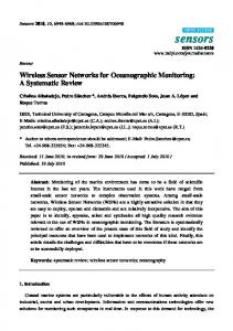
MATERIALS AND METHODS The experiments were conducted at the Conservation Production and Research Laboratory, Bushland, Texas (35° 11' N, 102° 06' W, 1174 m above mean sea level) where cotton (Gossypium hirsutum L.) varieties PayMaster 2280 and Delta Pine 117 B2RF were planted in 2007 and 2008, respectively, under ½ of a 6‐span center pivot field (11 ha) and 3‐span center pivot (2.8 ha). Both varieties were Bollgard II® Roundup Ready®. In 2007, we constructed circuit boards to interface an off‐the‐shelf infrared thermocouple thermometer with an off‐the‐shelf radio frequency (RF) module. These wireless sensors devices are referred to as sensor nodes and the first prototype was labeled Gen‐I. We improved the design of the initial sensor node prior to the second growing season (winter of 2008) by using surface mount components, a faster microprocessor with increased memory capacity, and switched to nickel metal hydride (NiMH) batteries to decrease battery pack size. The improved sensor node is referred to as Gen‐II. The remaining portion of the Materials and Methods section is divided into four parts. The first section describes only the design of the Gen‐II nodes since both were similar. The second section explains investigations performed to characterize the main effects of antenna type, antenna power level, sensor height, PVC housing, and location under the pivot lateral on radio frequency (RF) signal strength using loop‐back range tests in the field between individual sensor nodes and a RF modem (coordinator). The third section describes the wireless sensor networks (WSNs) that we established using the wireless sensor nodes and the system infrastructure to collect data from the WSNs to control and monitor movement of the center pivot system. WIRELESS SENSOR NODES The Gen‐II sensor nodes were of two types: a wireless infrared thermocouple thermometer (IRT) sensor node and a wireless GPS node. The nodes were constructed by interfacing an industrial IRT (IRT/c.5:1 type T‐80F/27C, Exergen, Watertown, Mass.) and a handheld GPS unit (WAAS enabled global positioning system, Garmin17HVS, Olathe, Kans.) with an 8‐bit PIC microcontroller, the PIC16F883 (Microchip Technology, Inc., Chandler, Ariz.), and a RF module (XBee platform: MaxStream, Logan, Utah). The microprocessor was programmed with PICBASIC PROTM Compiler (microEnginering Labs Inc., Colorado Springs, Colo.). Additional major components of the IRT sensor node included two MAX6674 (Maxim Integrated Products, Sunnyvale, Calif.) cold conjunction compensation (CJC) and analog‐to‐digital (AD) converters. One converter conditioned the analog signal from the infrared thermocouple thermometer and the second converter conditioned the signal from the type‐T thermocouple inserted into a mounting hole in the IRT body housing. A precision integrated circuit (IC) temperature sensor, the LM35 (National Semiconductor, Santa Clara, Calif.), was used to measure board temperature and the output was fed directly into the microprocessor for AD conversion. A recharge circuit with voltage and thermal cut‐off protection

Vol. 26(2): 331‐341

MAX6674 LM35

Whip antenna

XBee Module

Figure 1. Circuit interface for the wireless infrared thermocouple thermometer showing the main components and recharge circuit.

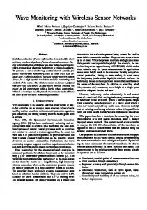
was constructed to recharge the batteries with a solar panel [Kyocera: 1.2 W, 12 V, Hudson, Mass. (fig. 1)]. The sleep pin on the RF module was controlled by the microprocessor. Desiccant packets were placed inside the weatherproof housing to absorb moisture from condensation. The sensor nodes were placed inside of white polyvinyl chloride (PVC) pipe, 50.8 mm in (diameter) × 178 mm (length) with a wall thickness of 3.2 mm, for weatherproofing and to reduce heat transfer due to direct radiation. Each sensor was powered individually by a nickel metal hydride battery pack and the batteries were recharged by a solar panel throughout the growing season. Data collected from each sensor node and the corresponding IC component and type of signal conditioning methods are summarized in table 1. ANTENNA SELECTION Range tests were conducted under the pivot prior to planting to investigate the impact of the ”pivot environment” on signal strength. We performed three replications of loop‐back tests at each of 11 radial distances and at two vertical heights above grade (table 2). The XBee coordinator was fixed at the pivot point while the sensor node was positioned under the pivot lateral. The sensor node was placed inside PVC housing (as previously described) and hung from a pole by a cord of adjustable length (fig. 2). The configuration and test utility software (X‐CTU, Digi International 2008. Ver. 5.1.4.1) was used to send 100 packets of data from the coordinator and monitor the return transmission rate from the sensor node. We used different heights to simulate the range of expected distances between the sensor node and the ground during the growing season, while adjusting for crop height. The power level (mW) for the XBee antennas was selected using X‐CTU software. Additionally, we used the same setup to determine the mean signal path loss associated with the PVC enclosure. Path loss was determined by reading the dB level at the coordinator after requesting a data transmission packet from a sensor node while the sensor and circuit board module were enclosed inside of PVC housing and then located outside of the housing. The sensor node was hung from a pole at 1.83 m above ground. Two different wireless sensor nodes were chosen at random and tested at three different separation

333

Table 1. Data collected at wireless sensor node. Component

Data Crop canopy temperature (Ts) Sensor body temperature (Tb) Battery voltage Node ID Board temperature Battery temperature

Signal Conditioning

Infrared thermometer Type‐T thermocouple inside mounting hole of IRT steel body chassis Voltage divider[c] (Vo = Vb *Ro/RT) RF address in EEPROM of PIC Precision LM35 IC[d] Thermistor

CJC[a], ADC[b]

Amplification, Amplification, CJC, ADC ADC N/A ADC ADC of voltage/ temperature

Units mV mV mV ASCII mV mV

[a] [b] [c]

CJC‐ cold junction compensation. ADC‐ analog to digital conversion. Vo = output voltage as a ratio of battery voltage, Vb, where Ro is the resistor that feeds a proportion of Vb to the microcontroller, and RT is the total resistance in the voltage divider circuit. [d] Integrated circuit where the analog output = 10 mv/°C. Table 2. Variables used in antenna evaluation. Antenna Characteristics Antenna type (in dBi Gain) RF power level (mW) Sensor height (m) Radial distance from pivot point (m)

Variables Dipole (2.0); Wire (1.8); Chip (‐1.5) 0 ( 1); 1 (16); 2 (25); 3 (32); 4 (40) 0.67; 1.83 15; 30; 45; 61; 77; 91; 106; 122;152;183; 213; 243; 260

distances from the coordinator. Ten transmission packets were sent from the sensor node at each distance. Antennas for both the sensor node and coordinator were maintained in the same horizontal plane. A third field test (DOY 168 and 175, 2009) was conducted to determine if there was a difference in signal path loss when a sensor node was located on the pivot lateral as compared to the field, 180° away from the pivot arm. The coordinator remained stationary and was located inside of a weatherproofed enclosure 1.83 m above ground level. We used a single sensor node and mounted it to the pivot lateral on a mast at seven different separation distances, 1.83 m above grade. The signal strength was measured at the coordinator using X‐CTU software after requesting 10 data transmission packets. This test was replicated 10 times at each separation distance.

NETWORK ARCHITECTURE To test the reliability of data transmission and compare mesh‐networking and non‐mesh networking protocols, two separate wireless sensor networks were established, the Pivot wireless sensor network (Pivot WSN) and the Field wireless sensor network (Field WSN). Both of the WSNs included a coordinator physically connected (via RS232 or Universal Serial Bus) to the embedded computer. Coordinators had the capability of selecting the channel and personal area network identification (PAN ID) and were powered continuously via their connection to the embedded computer. It was the coordinators that enabled routers and end‐devices with the same PAN ID configuration to join the network. A router is a transceiver that can function solely to route data, either from other end‐devices or other routers, or it can be a fully functioning sensor with a transceiver. The router must be joined to the Zigbee personal area network (PAN) before it can transmit, receive, or route data. After joining, it will allow other routers and end‐devices to join the network. Routers must also be powered constantly, and therefore cannot be configured to sleep. End‐devices are sensor nodes that must interact with a router or coordinator. Wireless sensor networks were assembled at the start of the growing season, one network was mounted on masts attached to the pivot arm of a center pivot irrigation system. Cord to suspend sensor node Sensor node platform w/RF module

Pole h = 1.83 m

Figure 2. Diagram depicting method used to position sensor node under the pivot lateral to perform the loop‐back range tests. The string suspending the sensor node housing was adjusted to 0.67 and 1.83 m.

334

APPLIED ENGINEERING IN AGRICULTURE

During the first growing season (2007), the XBee‐PRO OEM RF Series I moduleswere installed on all sensor nodes, however the FreeScale Zigbee enabled platform was limited in memory and hampered by software bugs, therefore these sensor nodes did not simultaneously support mesh‐ networking and cyclic sleep modes (T. Holman, personal communications, 15 June 2007). The Pivot WSN contained the GPS sensor node mounted on the end tower to improve the accuracy of position estimates of the center pivot using calibration methods by Peters and Evett (2005), and wireless IRT nodes to monitor crop canopy temperature while the pivot was moving (fig. 3a). All of these sensor nodes were configured with mesh‐networking firmware and programmed to sample 15 times min‐1 and transmit averaged values at the end of the minute to the base computer. A second network was constructed using wireless IRTs (IRT/c.5:1 type T‐80F/27C, Exergen, Watertown, Mass.) located on masts in the cropped field below the center pivot arm. The Field WSN, was stationary, and sensor nodes sampled crop canopy used as reference temperatures to estimate remote diurnal canopy temperatures when the pivot was moving; these reference temperatures were the means to determine one‐time‐of‐day temperature readings using the scaling method described by Peters and Evett (2004), figure 3b. These nodes were configured with non‐mesh firmware and sleep capability. Nodes were programmed for a 1‐s active time and transmitted data every minute.

Pivot Arm

Router

Mast

Sensor node

(a)

Mast External battery pack with solar

Wireless sensor node

(b) Figure 3. Photograph of: (a) wireless sensor network established on 6‐span pivot lateral; and (b) wireless sensor network established in the irrigated field.

Vol. 26(2): 331‐341

Each WSN contained a coordinator, the controlling device in a network, responsible for forming the network and allowing routers (transceivers), and sensor nodes (end devices) to associate with it. Both networks were established using a unicast transparent mode of communication. During each experiment, the height of the IRT sensor nodes was adjusted to maintain a minimum distance of 0.67 m above the crop canopy. For the 2008 growing season, the Series II XBee RF modules (based on the Ember EM250T system, available at: www.digi.com/news/pressrelease.jsp?prid=303, accessed 06 May 2008) were substituted for the Series I modules. The Series II RF microprocessor had an expanded memory, this in combination with new firmware allowed for the simultaneous implementation of mesh‐networking and cyclic sleep features. Gen‐II sensor nodes and the single GPS sensor node were again mounted onto the 6‐span center pivot in the same manner as 2007. The WSN was expanded to include four routers (transceivers only) located 0.3 m above the pivot pipeline at the high points between spans 1, 2, 3, and 6 to extend network coverage. Our goal was to minimize the separation distance between network devices to less than 31 m whenever possible. These routers were installed because pre‐season testing demonstrated that data transmission from the Pivot WSN (using Series II RF modules) was not as dependable as expected. The Field WSN again included 8 wireless IRT sensor nodes of which three functioned as routers. All three routers were outfitted with dipole antennas. Sampling rates and transmission frequency were modified from the previous season. The GPS sensor node sampled every 5 s, averaged data every minute, and transmitted RF data 5 s into the minute to the coordinator. The Gen‐II IRT nodes were coded to collect crop canopy, sensor body, and board temperature every 5 s, average and store this data every minute. Battery voltage and temperature were read and stored each min. These sensor nodes were programmed to transmit data every 10 min within a 10‐s active state (fig. 4). Mesh‐networking firmware was installed on RF modules for both WSNs. Also in 2008, 12 wireless Gen‐I sensors were placed on masts and located under a 3‐span center pivot system to provide stationary crop canopy reference temperature measurements. The data collection protocol was modified by broadcasting a special character through the coordinator to all nodes on the network, at the top of every minute. After receiving the special character, the microprocessor in each sensor node began sampling and accumulating data. An internally programmed time‐delay unique to each microprocessor offset the timing for the RF data packet to transmit to the coordinator. Sensor nodes used the unicast method to transmit data to the coordinator (fig. 5). The layouts and details of each of the WSNs in 2007 and 2008 are summarized in table 3. SYSTEM DESIGN Each WSN system was connected to an embedded computer (1U, Ampro Ready System, Ampro Computers, San Jose, Calif.) located at the pivot point. The embedded computer functioned as a supervisory control and data acquisition (SCADA) system. It was programmed using Microsoft Visual Studio 2005.Ver. 4.0. (Microsoft Corp., Redmond, Wash.) to capture RF data through the dedicated communications port for each WSN. The embedded

335

Power On Power on

Set all output variables and counter to zero Wake the RF module (pin controlled) Sample and accumulate data: Infrared thermometer readings Sensor body temperature Circuit board temperature

Listen for broadcasted code from WSN coordinator

No All samples taken within minute interval?

Special character received?

Yes Sample: Battery voltage Battery temperature Increment counter

Is counter equal to 10?

No

Yes Pause for a unique amount of time: Node ID * 100 millisec Accumulate 20 data samples from: IRT reading Sensor body temperature Battery voltage Send data to WSN coordinator Sleep the RF module Sleep microprocessor(time controlled)

No

Yes Wake RF module Send node ID Send data packets Sleep RF module

Figure 4. Algorithm for coding of the PIC microprocessor from the Gen II sensor nodes.

computer captured, parsed, time stamped, and applied calibration coefficients to the raw data. Air temperature, relative humidity, solar radiation, wind speed, and rainfall were measured at 6‐s intervals and reported as 15‐min mean values from a weather station located approximately 5 m from the pivot point. The weather data were transmitted wirelessly to the embedded computer using 900‐MHz radios. Finally, the embedded computer was serially linked to the pivot's controller, allowing for direct communication and control of the center pivot as reported by Evett et al. (2006). A wireless Ethernet connection (802.11A, frequency of 5800 MHz, channel = 64, and transmission power of 11 dBm) was the link between the embedded computer and desktop computers in our office (J. Ennis, personal communication, 26 June 2009) located approximately 2 miles away. This connection provided for review of the crop canopy temperature, the status of the

Figure 5. Algorithm for sensor node using the Basic Stamp as the microprocessor to manage data interface with the XBee RF module.

center pivot system, and remote control from our laboratory office (fig. 6). CALCULATIONS The influence of main effects on signal strength was analyzed using SAS (SAS Institute, Inc., Cary, N.C.) with a procedure for mixed models (PROC Mixed), and least significant difference method. Battery Life Optimization of a wireless self‐powered sensor node is often described in terms of battery life, which was calculated using equation 1 from Hebel (2006):

Table 3. Summary of wireless sensor networks. 2007 Network Configurations: Six‐span Center Pivot System Network

Location

Number of Sensor Nodes

Firmware (XBee Series)

Field‐WSN Pivot‐WSN

Six‐span center pivot: Stationary masts located in the field above crop canopy Six‐span center pivot: Masts located on pivot arm, forward of drop hoses

8 9

Non‐mesh (I) Mesh (I)

2008 Network Configurations

336

Network

Location

Number of Sensor Nodes

Firmware (XBee Series)

Field‐WSN WSN‐Pivot Field‐WSN

Six‐span center pivot: Stationary masts located in the field above crop canopy Six‐span center pivot: Masts located on pivot arm, forward of drop hoses Three‐span center pivot: Stationary masts located in the field above crop canopy

8 13 12

Mesh (II) Mesh (II) Non‐mesh (I)

APPLIED ENGINEERING IN AGRICULTURE

Pivot Wireless Sensor Networ k 2.4 GHz

GPS

Routers

Building Office

Weat her Station

900 MHz

5.8 G Hz 802.11

Field Coordinator

Field Wireless Sensor Network 2.4 GHz

Embedded Computer

Pivot Coordinator

Figure 6. Supervisory control and data acquisition system for center pivot control and automation: where the embedded computer is located inside a weather closure powered by 12V AC. The Field and Pivot Coordinators are wired to the embedded computer through USB cables, while the control panel of the center pivot is connected via a RS‐232 cable. Data from the sensor nodes on the Pivot and Field WSN are transmitted in the 2.4‐GHz range. The wireless connection from the embedded computer from the weather station and Ethernet connections are shown as dashed lines to illustrated these a separate networks on different frequencies (900 MHz between the weather station and 5.8 GHz for the Ethernet connection from the office building to the pivot point).

L=

C Is + D* Ia

(1)

where L is the life of the battery (h), C is battery capacity (mAh), Is is the quiescent current (mA), D is the duty cycle (%), and Ia (mA) is the current draw when the sensor node is actively transmitting or receiving data. Evaluating Data Transmission An equation similar to that of Andrade‐Sanchez et al. (2007) was used to quantify the performance of the Pivot and Field WSNs. We defined the success of transfer of data packets (bytes of information) as a percentage: ⎡ RR x ⎤ PRPx = ⎪ ⎥100 ⎣ TR x ⎦

(2)

where PRPx was the packet reception percentage, RRx was the number of records received during the time interval x, and TRx was the total number of records transmitted during the interval time x. Each WSN transmitted data on its own

specified channel to a specific coordinator. The PRP was compared between the Pivot and Field WSNs using SAS and mixed model methods.

RESULTS TRANSMISSION RATE AND CALCULATED BATTERY LIFE The quiescent current of the wireless sensors nodes was verified by sampling 10% (n = 5) of our inventory while the XBee RF module was in the “sleep” state and all other ICs were powered; the mean quiescent current was 45.2 ± 1.6 mA, and 2.4 ± 1.3 mA for the first and second generation nodes, respectively. Battery life for the different network nodes was calculated using equation 1. The sleep mode used with the Gen‐I nodes reduced the duty cycle by 98% and doubled the battery life. Gen‐II sensor nodes that functioned as routers were powered continuously, limiting their battery life considerably. Configuring these same nodes with a sleep mode increased the calculated battery life by 15‐fold (table 4).

Table 4. Calculated battery life of wireless sensor node prototypes.

Network Device IRT Node ‐ Gen I, Mesh networking, no sleep capability IRT Node ‐ Gen I, Non‐mesh networking, with sleep capability Router, Gen II with sensing capability, always `awake' IRT Node ‐ Gen II, Mesh networking and sleep capability [a] [b] [c]

Battery Capacity (mAh)

Quiescent[a] Current (mA)

Active[b] Current (mA)

Active[c] Time (min)

Duty Cycle (%)

Battery Life (h)

4000 4000 1800 1800

45.2 45.2 2.4 2.4

65.0 65.0 45.0 45.0

1440 24 1440 24

100 1.67 100 1.67

36 87 38 570

Current draw when the node is not transmitting or listening; the RF module is in the sleep state. Current draw when the node is transmitting or receiving. Number of minutes within a 24‐h period in which the node is transmitting or receiving.

Vol. 26(2): 331‐341

337

Antenna Characteristics Proc mixed analysis with SAS software was used to quantify the main effects of antenna type, horizontal distance between transceivers, vertical distance above finished grade, and antenna power level on percent transmission of 100 data packets during the loop‐back range test. All of the main effects had a significant impact on PRP. The Chip antenna demonstrated limited reliability after a separation distance of 100 m regardless of the power level setting and its height above ground. The range of the wire whip and omni‐dipole antennas were consistently high (> 90%) for all measured distances when their power levels were set at 3 and 4 (32 and 40 mW), respectively (table 5). Increasing the antenna above grade level demonstrated a statistically significant improvement in PRP, while as expected, an increase in separation range for any antenna type resulted in a decrease in PRP. Raising the radio power level above `2' did not significantly affect PRP results. PVC Housing Testing demonstrated that the PVC housing, used to weatherproof the sensor nodes, significantly attenuated the RF signal. The difference in the means of the received signal strength indicator (RSSI, measured in dB) for the two sensor Table 5. Main effects impacting packet reception percentage.[a] Factor

Average PRP (%)

Antenna Omni Wire Chip

79.0 a 82.8 b 52.4 b

Radio power[b] 0 1 2 3 4

47.5 a 69.1 b 77.1 b, c 82.1 c 80.4 c

Height above grade (m) 0.67 1.83

60.1 a 75.3 b

Separation distance[c] (m) 15 30 45 61 77 91 106 122 152 183 213 243 260

98.4 a 97.2 a 96.9 a 91.2 a 85.2 a,b 83.2 a,b 71.2 b,d 62.3 b,c,d 61.7 b,c,d 56.9 c,d 51.5 c,e 37.8 e,f 32.9 f

[a]

Means in columns with the same letters are not significantly different from one another. [b] See table 2 for description of power level in mW. [c] Distance between transmitter and receiver.

338

nodes at each of five separation distances was analyzed using the least significant difference method. The mean signal path loss and standard deviation for the sensors located in PVC housing were 2.85 ± 2.1 dB (sensor α) and 2.75 ± 1.3 dB (sensor β). The mean signal loss was less than results (3.5 dB) measured by Darr and Zhao (2008) using PVC of similar wall thickness, but since a spectrum analyzer was not available to us; accuracy was limited to the capabilities of the RF module. Proximity to Pivot Lateral The investigation to quantify the impact of the pivot's structure on signal attenuation for sensor nodes located on the pivot arm produced mixed results. The signal strength measured between a coordinator and a sensor node located under the pivot lateral (attached to a mast off the pivot arm) and then with the same node located 180° away from the pivot lateral was significantly different at separation distances of 45 and 60 m (fig. 7a). At these distances, the mean loss differences were 9.0 and 5.2 dB greater when the sensor node was located under the pivot lateral. However, at all other separation distances (52, 75, 105, 116, and 150 m) the signal strength was not significantly different (table 6). A second similar test was conducted on a DOY 175 (2009). The signal strength was significantly less when the sensor node was located under the pivot lateral versus its location in the field, 180° away from the pivot arm. The mean loss differences were 5.9, 7.8, and 9.1 dB for the separation distances of 39, 56, and 67 m, respectively. There was no significant difference in RSSI at 97 m (fig. 7b). High variability occurred at the shortest separation distance between the coordinator and sensor node device. The results of these tests indicate that signal path loss at shorter separation distances between the coordinator (located at the pivot point) and a network device are more likely to occur when the network device is located on the pivot lateral. Losses were due to the “environment under the pivot” which can include reflection by the pivot point frame, the first drive tower, the terrain, and metal masts supporting the wireless sensor node devices. Darr and Zhao (2008) showed similar results of signal attenuation in a CAFO environment, and they determined that signal reflection off surfaces resulted in significant attenuation. Andrade‐Sanchez et al. (2007) showed that line of sight alone was not the only consideration influencing signal strength, but rather spatial arrangement of the network in terms of horizontal and vertical planes and obstacles within the Fresnel zone of the transmitting sensor nodes affected RSSI. IMPACTS ON PERCENT PACKET RECEPTION RATE (NETWORK PERFORMANCE) The average PRP for wireless sensor nodes on each of the two networks was determined for a 15‐day period and compared using Proc Mixed models. Nodes on the Field WSN consistently had a higher PRP than the nodes on the Pivot WSN in the case of non‐mesh networking (2007) and mesh‐networking (2008) protocols (table 7). The average time to collect data reliably from a single sensor was 8 and 32 s from sensors on the Field and Pivot WSNs, respectively. Automatic time stamps that were imposed when collecting data from the sensor nodes in 2007 for DOY 208, 209, and 210 provided this information. The first time stamp was recorded at the start of polling and the second time stamp was

APPLIED ENGINEERING IN AGRICULTURE

-70

Table 7. Percent reception percentage results from deployed wireless networks.[a]

-75

Sensors on Pivot Lateral

RSSI (dB)

-80

2007 Wireless Sensor Networks

Sensors in Field

Network System (no. of nodes)

Communication

Avg. Packet Reception Percentage

Pivot‐WSN (9) Field‐WSN (8) Pivot‐WSN (9)

Unicast, mesh‐networking Unicast, non‐mesh networking Unicast, non‐mesh networking

84.2 a 94.0 b 87% for the Pivot WSN and approximately 94% for the Field WSN during the irrigation season. This was an improvement over the performance of both networks during the previous growing season. However, data dropout persisted on the Pivot WSN even with routers installed on the pivot lateral. The benefits of mesh‐networking were that it provided for ad‐hoc data transmission and eliminated the need to poll sensor nodes individually. Ultimately, mesh‐networking has the potential to lead to true plug‐and‐play architecture for WSNs in agricultural applications. A plug‐and‐play system will allow for easier system set‐up and configuration, more accurate sensor data management, easier operation, and less maintenance for the farmer. Other improvements that we made to address performance issues included shortening the amount of bytes transmitted from each sensor by using API (Applications Programmer's Interface) mode to structure data streams more efficiently, transmitting less data, and using algorithms to interpolate dropped data points. ERROR CHECKING Inclusion of the IRT node ID and the checking of correct packet size at the embedded computer provided redundancy to ensure that the RF data was not fragmented or combined with data from another sensor node.

CONCLUSIONS This study demonstrated that wireless IRT sensor nodes could be developed by interfacing electronic circuit boards with off‐the‐shelf industrial products to provide reliable remote data acquisition of crop canopy temperatures over a growing season. In addition, it was demonstrated that wireless mesh‐networking sensors could function in a challenging environment, such as on a moving sprinkler

339

irrigation system. Mesh‐networking, frequent data sampling, intermittent RF transmissions, and algorithms to perform error checking and handle dropped data were all critical components to attain reliable wireless supervisory control of the pivot. The technology for establishing wireless IRT networks can be transferred to other types of sensors and utilized in gathering feedback for agricultural applications. Complete success will require a solution to the presence of plant or mechanical obstructions that may reflect RF signals. Further work needs to be accomplished towards reducing the cost of the wireless sensor nodes, which in our case is the substitution of an inexpensive but precise IR photo‐detector for the industrial grade IRT that we are currently using, perhaps one that is similar to one tested by Mahan and Yeater (2008). Additional improvements are needed at the RF software level to further stabilize network association. Communication to that effect must continue with the manufacturer of the RF modules to ensure that improvements are brought to the retail sector. Although we increased the battery life of our sensors, mainly by reducing the quiescent current, battery longevity without supplementary recharge should be increased to at least six to eight months. Future studies need to address the reduction of quiescent current draw by testing the performance of switching voltage regulators and optimizing cyclic sleep and data transmission patterns. Battery longevity should be tested with the revised sensor nodes deployed in the field without solar panel recharge. ACKNOWLEDGEMENTS The authors wish to acknowledge funding from the Ogallala Aquifer Program and from a joint grant from the Bilateral Agricultural Research and Development (BARD) fund and Texas Department of Agriculture (grant no. TIE04‐01). We also acknowledge with great appreciation the assistance provided by Chad Ford, Agricultural Science Technician, and Brice Ruthardt, Biological Science Technician.

REFERENCES Abad, E., F. Palacio, M. Nuin, A. González de Zárate, A. Juarros, J. M. Gómez, and S. Marco. 2009. RFID smart tag for traceability and cold chain monitoring of foods: Demonstration in an intercontinental fresh fish logistic chain. J. Food Eng. 93(4): 394‐399. Adya, A., P. Bahl, J. Padhye, A. Wolman, and L. Zhou. 2004. A multi‐radio unification protocol for IEEE 802.11 Wireless Networks. In Proc. 1st Intl. Conf. on Broadband Networks, 344‐354. San Jose, Cal.: IEEE. Ajayi, A. E., and A. A. Olufayo. 2004. Evaluation of two temperature stress indices to estimate grain sorghum yield and evapotranspiration. Agron J. 96(5): 1282‐1287. Akyildiz, I. F., X. Wang, and W. Wang. 2005. Wireless mesh networks: A survey. Computer Networks 47(4): 445‐487. Andrade‐Sanchez, P., F. J. Pierce, and T. V. Elliott. 2007. Performance assessment of wireless sensor networks in agricultural settings. ASABE Paper No. 073076. St. Joseph, Mich.: ASABE. Alves, I., and L. S. Pereira. 2000. Non‐water‐stressed baselines for irrigation scheduling with infrared thermometers: A new approach. Irrig. Sci. 19(2): 101‐106. Ben‐Asher, J., C. J. Phene, and A. Kinati. 1992. Canopy temperature to assess daily evapotranspiration and management

340

of high frequency drip irrigation systems. Agric. Water Man. 22(4): 379‐390. Chao, H., M. Baumann, A. Jensen, Y. Chen, Y. Cao, W. Ren, and M. McKee. 2008. Band‐reconfigurable multi‐UAV‐based cooperative remote sensing for real‐time water management and distributed irrigation control. In Proc. The Intl. Federation of Automatic Control, 11744‐11749. Seoul, Korea: IFAC. Clawson, K. L., and B. L. Blad. 1982. Infrared thermometry for scheduling irrigation of corn. Agron. J. 74(2): 311‐316. Colaizzi, P. D., E. M. Barnes, T. R. Clarke, C. Y. Choi, and P. M. Waller. 2003a. Estimating soil moisture under low frequency surface irrigation using crop water stress index. J. Irrig. and Drain. Eng. 129(1): 27‐35. Colaizzi, P. D., E. M. Barnes, T. R. Clarke, C. Y. Choi, P. M. Waller, J. Haberland, and M. Kostrezewski. 2003b. Water stress detection under high frequency sprinkler irrigation with water deficit index. J. Irrig. and Drain. Eng. 129(1): 36‐43. Darr, M. J., and L. Zhao. 2008. A wireless data acquisition system for monitoring temperature variations in swine barns. In Livestock Environment VIII, Proceedings of the International Symposium, 987‐994. St. Joseph, Mich.: ASABE. Dowla, F. 2006. Handbook of RF and Wireless Technologies. Burlington, Mass.: Elsevier Science. Evett, S. R., T. A. Howell, A.D. Schneider, D. R. Upchurch, and D. F. Wanjura. 1996. Canopy temperature based automatic irrigation control. In Proc. Intl. Conf. Evapotranspiration and Irrigation Scheduling, 207‐213. C. R. Camp, E. J. Sadler, and R. E. Yoder, eds. San Antonio, Tex.: ASAE. Evett, S. R., R. T. Peters, and T. A. Howell. 2006. Controlling water use efficiency with irrigation automation: Cases from drip and center pivot irrigation of corn and soybean. In Proc. 28th Annual Southern Conservation Systems Conf., 57‐66. Amarillo, Tex.: SCSC. Falkenberg, N. R., G. Piccinni, T. Cothren, D. I. Leskovar, and C. M. Rush. 2007. Remote sensing of biotic and abiotic stress for irrigation management of cotton. Agric. Water Mgmt. (87): 23‐31. Frenzel, L. E. 2007. Do‐it‐yourself wireless design. Electronic Design 55(20): 57‐62. Goense, D., and J. Thelen. 2005. Wireless sensor networks for precise phytophthora decision support. ASABE Paper No. 053099. St. Joseph, Mich.: ASABE. Gonda, L., and C. E. Cugnasca. 2006. A proposal of greenhouse control using wireless sensor networks. In Computers in Agriculture and Natural Resources, 4th World Congress, Proc. of the Intl. Conf., 229‐233. St. Joseph, Mich.: ASABE. Guo, L. S., and Q. Zhang. 2005. Wireless data fusion system for agricultural vehicle positioning. Biosystems Eng. 91(3): 261‐269. Harms, T. E. 2005. Soil moisture based web to wireless center pivot operation. 2005 Pacific Northwest section meeting. ASAE Paper No. PNW05‐1003. St. Joseph, Mich.: ASAE. Hebel, M. A. 2006. Meeting wide‐area agricultural data acquisition and control challenges through Zigbee wireless network technology. ASABE Paper No. 701P060. St. Joseph, Mich.: ASABE. Howell, T. A., J. L. Hatfield, H. Yamada, and K. R Davis. 1984. Evaluation of cotton canopy temperature to detect crop water stress. Trans. ASAE 27(1): 84‐88. Humphreys, A. S., and H. D. Fisher. 1995. Water sensor feedback control system for surface irrigation. Appl. Eng. in Agric. 11(1): 61‐65. IEEE802.11. 2007. Standard for information technology‐ telecommunications and information exchange between systems‐Local and metropolitan area networks‐Specific requirements ‐ Part 11: Wireless LAN Medium Access Control (MAC) and Physical Layer (PHY) Specifications, 2007. Available at: standards.ieee.org/getieee802/802.11.html. Accessed 15 September 2008.

APPLIED ENGINEERING IN AGRICULTURE

IEEE802.15.1. 2005. Part 15.1: Wireless Medium Access Control (MAC) and Physical Layer (PHY) Specifications for Wireless Personal Area Networks (WPANs(tm)), 2005. Available at: standards.ieee.org/getieee802/download/802.15.1‐2005_part1. Accessed 15 September 2008. IEEE802.15.4. 2007. Specific requirements Part 15.4: Wireless Medium Access control (MAC) and Physical Layer (PHY) Specifications for Low‐Rate Wireless Personal Area Networks (WPANs). Amendment 1: Add Alternate PHYs. IEEE, Inc., 3 Park Avenue, New York, NY Available at: standards.ieee.org/ getieee802/802.15.html. Accessed 15 September 2008. Irmak, S., D. Z. Haman, and R. Bastug. 2000. Determination of crop water stress index for irrigation timing and yield estimation of corn. Agron J. 92(6): 1221‐1227. Jackson, R. D., R. J. Reginato, and S. B. Idso. 1977. Wheat canopy temperature: A practical tool for evaluation water requirements. Water Resour. Res. 3(13): 651‐656. Jackson, R. D., S. B. Idso, R. J. Reginato, and P. J. Pinter. 1981. Canopy temperature as a crop water stress indicator. Water Resour. Res. 17(4): 1133‐1138. Jedermann, R. L. Ruiz‐Garcia, and W. Lang. 2009. Spatial temperature profiling by semi‐passive RFID loggers for perishable food transportation. Comput. Electron. in Agric. 65(2): 145‐154. Kim, Y., R. G. Evans, and W. M. Iversen. 2008. Remote sensing and control of an irrigation system using a distributed wireless sensor network. IEEE Trans. Instrum. Meas. 57(7): 1379‐1387. King, B. A., R. W. Wall, and L. R. Wall. 2005. Distributed control and data acquisition system for closed‐loop site‐specific irrigation management with center pivots. Appl. Engr. in Agric. 21(5): 871‐878. Mahan, J. R., J. J. Burke, D. F. Wanjura, and D. R. Upchurch. 2005. Determination of temperature and time threshold for BIOTIC irrigation of peanut on the Southern High Plains of Texas. Irrig Sci. 23(4): 145‐152. Mahan, J. R., and K. M. Yeater. 2008. Agricultural applications of a low‐cost infrared thermometer. Computers and Electron. in Agric. 64(2): 262‐267. McNair, J. Y. 2006. Chapt. 2: Next generation wireless networks. In Handbook of Wireless and RF Technologies, 23‐56. F. Dowla, ed. Burlington, Mass.: Elsevier Inc. Morais, R., M. A. Fernandes, S. G. Matos, C. Serodio, P. J. Ferreira, and M. J. Reis. 2008. A Zigbee multi‐powered wireless acquisition device for remote sensing applications in precision viticulture. Comp. Electron. in Agric. 62(2): 94‐106. Peters, R. T., and S. R. Evett. 2004. Modeling diurnal canopy temperature dynamics using one‐time‐of‐day measurements and a reference temperature curve. Agron. J. 96(6): 1553‐1561.

Vol. 26(2): 331‐341

Peters, R. T., and S. R. Evett. 2005. Using low‐cost GPS receivers for determining field position of mechanized irrigation systems. Applied Engr. in Agric. 21(5): 841‐845. Peters, R. T., and S. R. Evett. 2007. Spatial and temporal analysis of crop conditions using multiple canopy temperature maps created with center‐pivot‐mounted infrared thermometers. Trans. ASABE 50(3): 919‐927. Peters, R. T., and S. R. Evett. 2008. Automation of a center pivot using the temperature‐time‐threshold method of irrigation scheduling. J. Irrig. and Drainage Eng. 134(1): 286‐291. Pierce, F. J., J. L. Chavez, T. V. Elliott, G. R. Matthews, R. G. Evans, and Y. Kim. 2006. A remote‐real‐time continuous move irrigation control and monitoring system. ASABE Paper No. 062162. St. Joseph, Mich.: ASABE. Pierce, F. J., and T. V. Elliott. 2008. Regional and on‐farm wireless sensor networks for agricultural systems in Eastern Washington. Comp. Electron. in Agric. 61(1): 32‐43. Pinter, P. J., K. E. Fry, G. Guinn, and J. R. Mauney. 1983. Infrared thermometry: A remote sensing technique for predicting yield in water‐stressed cotton. Agric. Water Mgmt. 6(4): 385‐395. Poor, R. D. 2006. Chapt. 13: Reliable wireless networks for industrial applications. In Handbook of RF and Wireless Technologies, 311‐329. F. Dowla, ed. Burlington, Mass.: Elsevier Inc. Sadler, E. J., C. R. Camp, D. E. Evans, and J. A. Millen. 2002. Corn canopy temperatures measured with a moving infrared thermometer array. Trans. ASAE. 45(3): 581‐591. Stone, M. L., K. D. McKee, C. W. Formwalt, and R. K. Benneweis. 1999. ISO 11783: An electronic communications protocol for agricultural equipment. In Proc. ASAE Agricultural Equipment Technology Conf. ASAE Paper No. 913C1798. St. Joseph, Mich.: ASAE. Vellidis, G., M. Tucker, C. Perry, C. Kvien, and M. Tucker. 2007. How wireless will change agriculture. In Proc. the 6th European Conf. on Precision Agriculture, 57‐67. J. V. Stafford, ed. Skiathos, Greece: Wageningen Academic Publishers. Wang, N., N. Zhang, and M. Wang. 2006. Wireless sensors in agriculture and food industry: Recent development and future perspective. Comp. Electron. in Agric. 50(1): 1‐14. Wanjura, D. F., and D. R. Upchurch. 2000. Canopy temperature characterizations of corn and cotton water status. Trans ASAE 43(4): 867‐875. Wanjura, D. F., S. J. Mass, J. C. Winslow, and D. R. Upchurch. 2004. Scanned and spot measured canopy temperatures of cotton and corn. Comp. Electron. in Agric. 44(1): 33‐48. Zhang, Z. 2004. Investigation of wireless sensor networks for precision agriculture. ASAE/CSAE Paper No. 041154. St. Joseph, Mich.: ASAE.

341

342

APPLIED ENGINEERING IN AGRICULTURE