Development of a Propositionalization Toolbox - Computing ...

Development of a Propositionalization Toolbox

A thesis submitted in partial fulfillment of the requirements for the degree of Master of Science in Applied Computer Science at the University of Freiburg by

Peter Reutemann

Department of Computer Science Freiburg, Germany

Department of Computer Science Hamilton, New Zealand, Aotearoa

23 June, 2004

I declare that I did not draw up the whole thesis nor parts of it for another fulfillment of the requirements of the degree of Master of Science in Applied Computer Science at the University of Freiburg. Further I declare that I worked autonomously and only used the stated resources. All excerpts cited from publications or unpublished scripts are indicated. Hamilton, 23 June, 2004

There is a theory which states that if ever anyone discovers exactly what the Universe is for and why it is here, it will instantly disappear and be replaced by something even more bizarre and inexplicable.

There is another theory which states that this has already happened. — Douglas Adams

Acknowledgements Even though I did write this thesis alone there were still a lot of other people involved for getting it on the way... Foremost I want to thank my supervisors Dr. Eibe Frank and Dr. Bernhard Pfahringer, who really did a great job in guiding me through this time, but also letting me explore my own ideas. Even though our meetings sometimes looked like a tribunal to me, they were always fruitful and inspiring. I could always get handy advice regarding problems I encountered during the development of my project. The working environment of the Machine Learning group here at Waikato University is a reason to extend my stay here in New Zealand: it’s outstanding. Thanks to that you can even manage to slave away day and night in a windowless lab... Furthermore I am grateful to Professor Luc De Raedt, head of the Machine Learning group at the University of Freiburg, for offering me the opportunity to stay at the University of Waikato and co-supervising this thesis. I also wish to thank Associate Professor Geoff Holmes for providing the opportunity to German students to write their thesis at the Waikato Machine Learning group. In addition, I am very thankful for the financial support I received from the University of Waikato. For getting this thesis started I owe one to Mark-A. Krogel, Otto-von-Guericke-Universität ˇ in Magdeburg/Germany, and Filip Zelezn´ y, Czech Technical University in Prague/Czech Republic, for letting me use their source code and/or datasets. Last but not least, I would like to thank all the people I met in New Zealand who became dear to me. They helped me to find my way (on the “right” side of the road) in this country and motivated and supported me during my thesis. In particular I would like to mention: Stefan Mutter, Greger Burman, Ingmar Kühn, Nicole ”Essen” Urban, Professor Wilhelm Steinbuß, Tillmann Böhme, Anke Löhlein, the Kiwi Dale ”Auf Lederhosen” Fletcher and of course PG for the highlight of the day.

Contents

List of Figures

iii

List of Tables

v

1

Introduction

1

1.1

Relational Learning . . . . . . . . . . . . . . . . . . . . . . . . . . . . . .

2

1.2

Multi-Instance Learning . . . . . . . . . . . . . . . . . . . . . . . . . . .

5

1.3

Propositional Learning . . . . . . . . . . . . . . . . . . . . . . . . . . . .

6

2

3

Proper

7

2.1

Import . . . . . . . . . . . . . . . . . . . . . . . . . . . . . . . . . . . . .

7

2.2

Propositionalization and Conversion into Multi-Instance Data . . . . . . . .

12

2.2.1

RELAGGS . . . . . . . . . . . . . . . . . . . . . . . . . . . . . .

13

2.2.2

Joiner . . . . . . . . . . . . . . . . . . . . . . . . . . . . . . . . .

16

2.2.3

REMILK . . . . . . . . . . . . . . . . . . . . . . . . . . . . . . .

17

2.3

Export . . . . . . . . . . . . . . . . . . . . . . . . . . . . . . . . . . . . .

18

2.4

Tools . . . . . . . . . . . . . . . . . . . . . . . . . . . . . . . . . . . . . .

18

2.4.1

Relations . . . . . . . . . . . . . . . . . . . . . . . . . . . . . . .

19

2.4.2

Experiments . . . . . . . . . . . . . . . . . . . . . . . . . . . . .

20

2.4.3

Viewing ARFF files . . . . . . . . . . . . . . . . . . . . . . . . .

21

2.4.4

Distributed Experiments . . . . . . . . . . . . . . . . . . . . . . .

21

Related Work

29

3.1

MIWrapper . . . . . . . . . . . . . . . . . . . . . . . . . . . . . . . . . .

29

3.2

RSD . . . . . . . . . . . . . . . . . . . . . . . . . . . . . . . . . . . . . .

30

3.3

SINUS . . . . . . . . . . . . . . . . . . . . . . . . . . . . . . . . . . . . .

31

3.4

Stochastic Discrimination . . . . . . . . . . . . . . . . . . . . . . . . . . .

32

i

4 Experiments

35

4.1

Datasets and Settings . . . . . . . . . . . . . . . . . . . . . . . . . . . . .

35

4.2

Results . . . . . . . . . . . . . . . . . . . . . . . . . . . . . . . . . . . . .

39

4.2.1

Setting 1 . . . . . . . . . . . . . . . . . . . . . . . . . . . . . . .

39

4.2.2

Setting 2 . . . . . . . . . . . . . . . . . . . . . . . . . . . . . . .

41

4.2.3

Setting 3 . . . . . . . . . . . . . . . . . . . . . . . . . . . . . . .

43

4.2.4

Setting 4 . . . . . . . . . . . . . . . . . . . . . . . . . . . . . . .

45

4.2.5

Setting 5 . . . . . . . . . . . . . . . . . . . . . . . . . . . . . . .

47

4.2.6

Setting 6 . . . . . . . . . . . . . . . . . . . . . . . . . . . . . . .

49

4.3

Comparison of RELAGGS and Joiner . . . . . . . . . . . . . . . . . . . .

51

4.4

Tree sizes and runtimes . . . . . . . . . . . . . . . . . . . . . . . . . . . .

51

4.5

Summary . . . . . . . . . . . . . . . . . . . . . . . . . . . . . . . . . . .

55

5 Conclusion and Future Work

57

A Implementation

61

A.1 Execution . . . . . . . . . . . . . . . . . . . . . . . . . . . . . . . . . . .

61

A.2 Class Diagrams . . . . . . . . . . . . . . . . . . . . . . . . . . . . . . . .

65

A.3 Development . . . . . . . . . . . . . . . . . . . . . . . . . . . . . . . . .

90

B Proper Manual

91

B.1 Main Menu . . . . . . . . . . . . . . . . . . . . . . . . . . . . . . . . . .

91

B.2 First Steps . . . . . . . . . . . . . . . . . . . . . . . . . . . . . . . . . . . 101 C Datasets

121

Bibliography

123

ii

List of Figures

1.1

Proper from a logical perspective. . . . . . . . . . . . . . . . . . . . . . .

2

2.1

Proper from the program perspective. . . . . . . . . . . . . . . . . . . . .

7

2.2

Overview of the Import in Proper. . . . . . . . . . . . . . . . . . . . . . .

8

2.3

Example of the East-West-Challenge ( c represents the car and l the load). .

8

2.4

East-West-Challenge in a logical representation. . . . . . . . . . . . . . . .

9

2.5

East-West-Challenge as relational database. . . . . . . . . . . . . . . . . .

9

2.6

The post-processing of imported data in detail. . . . . . . . . . . . . . . . .

10

2.7

Different settings for Alzheimer/less toxic: first argument as key, two keys symmetric, two keys asymmetric. . . . . . . . . . . . . . . . . . . . . . . .

12

2.8

East-West-Challenge joined for RELAGGS. . . . . . . . . . . . . . . . . .

17

2.9

East-West-Challenge joined for MI learner. . . . . . . . . . . . . . . . . .

17

2.10 Relations - tool for exploring the relations in a database. Here a user defined tree is displayed for an Alzheimer dataset. With the max. Depth option the user can let Proper suggest a relation tree that can be edited afterwards. . .

19

2.11 Relation tree for the East-West-Challenge, where c represents a car and l the corresponding load . . . . . . . . . . . . . . . . . . . . . . . . . . . .

19

2.12 Excerpt of an ANT file generated with the Builder (the “...” denotes omissions). . . . . . . . . . . . . . . . . . . . . . . . . . . . . . . . . . . . . .

20

2.13 Builder - enables the user to build arbitrary experiments. . . . . . . . . . .

21

2.14 ArffViewer - for viewing and editing ARFF files. . . . . . . . . . . . . . . .

22

2.15 Basic overview of the Client-Server-Architecture. . . . . . . . . . . . . . .

22

2.16 Example run of the distributed experiments. . . . . . . . . . . . . . . . . .

23

2.17 Simple and extended synchronization scheme. . . . . . . . . . . . . . . . .

25

2.18 Visualization of the extended synchronization scheme as “dripping apparatus”. 25 2.19 Screenshot of the Jobber front-end. . . . . . . . . . . . . . . . . . . . . . . iii

26

2.20 Interaction of the JobMonitor with the JobServer and JobClients. . . . . . .

27

3.1

Artificial Dataset. . . . . . . . . . . . . . . . . . . . . . . . . . . . . . . .

30

3.2

Chemical fragment C-C=C . . . . . . . . . . . . . . . . . . . . . . . . . .

32

3.3

Chemical fragment as SQL query. . . . . . . . . . . . . . . . . . . . . . .

33

3.4

Graphical representation of the SQL query - the bond predicate is split into two, since it contains two atoms (the split id identifies the entries that belong together). The grey boxes depict the building blocks for longer and branched fragments . . . . . . . . . . . . . . . . . . . . . . . . . . . . . .

34

4.1

Comparison for Setting 1. . . . . . . . . . . . . . . . . . . . . . . . . . . .

40

4.2


42

4.3


44

4.4


46

4.5


48

4.6


50

4.7

Performance comparison of RELAGGS and Joiner on the Alzheimer dataset (the suffices indicate the step referenced in the text). The used classifier was the tree-classifier J48 with default values. . . . . . . . . . . . . . . . . . .

52

A.1 General overview of the flow of parameters inside the framework. . . . . .

62

A.2 Execution of a command line Application. . . . . . . . . . . . . . . .

62

A.3 Execution of a CommandLineFrame - the execution of an Engine is omitted. . . . . . . . . . . . . . . . . . . . . . . . . . . . . . . . . . . . .

iv

63

List of Tables

1.1

First-Order-Logic and Database terms. . . . . . . . . . . . . . . . . . . . .

3

2.1

DTDs and examples of messages sent between JobServer and JobClient(s).

24

3.1

Unpruned decision trees for the artificial dataset, containing 4 bags with 4 instances each. . . . . . . . . . . . . . . . . . . . . . . . . . . . . . . . .

4.1

Overview of the produced data, where each column shows the values for RELAGGS/Joiner/REMILK. . . . . . . . . . . . . . . . . . . . . . . . . .

4.2

37

Settings for the experiments. In case of multi-instance data the MIWrapper was used with default parameters. . . . . . . . . . . . . . . . . . . . . . .

4.3

30

37

Different behavior of the original NominalToBinary filter and the modified version, if nominal attribute contains only two distinct values (“att” is the name of the example attribute). Missing values are replaced with “0”. . . .

37

4.4

Accuracy and standard deviation for Setting 1. . . . . . . . . . . . . . . . .

40

4.5


42

4.6


44

4.7

Overview of portion of attributes with missing values in the alzheimer toxic, genes growth and thrombosis multi-instance datasets (generated with the Joiner). It is checked how many attributes (in percent) have a percentage of missing values above a certain threshold. This is done for All attributes and only for Nominal ones. . . . . . . . . . . . . . . . . . . . . . . . . . . . .

44

4.8


46

4.9


48

4.10 Accuracy and standard deviation for Setting 6. . . . . . . . . . . . . . . . .

50

v

4.11 Tree size for AdaBoostM1/pruned J48 averaged over 10 iterations (only datasets with results for all three approaches were considered for the “Smallest Tree” count). . . . . . . . . . . . . . . . . . . . . . . . . . . . . . . . .

53

4.12 Runtimes in seconds for AdaBoostM1/pruned J48 (i.e. time to build the classifier for printing the tree and to execute 10 runs of 10-fold CV). Only datasets with results for all three approaches were considered for the “Fastest” count. . . . . . . . . . . . . . . . . . . . . . . . . . . . . . . . . . . . . .

54

4.13 Runtimes in seconds for different database systems (Imp. = Import, REL = RELAGGS, Joi. = Joiner, REM = REMILK). Note: “col” means that too many columns were produced (but not necessarily a program termination), “abort” that the process was aborted, because consuming too much time, and “-” that the process was not executed at all. . . . . . . . . . . . . . . . . . . . . . . . .

vi

54

Chapter 1 Introduction

Zwar weiss ich viel, doch möcht’ ich alles wissen. (And so I know much now, but all I fain would know.)

— Wagner in Goethe’s Faust

Are you using a reward card like Miles-and-More, Fly Buys or do you own a shopping card? Did you ever get “junk-mail” from the companies participating in that reward system? Did you ever wonder why their recommendations were so specific? What they do is building up a profile from all the purchases you do, from the preferences you enter on their websites, the websites you visit. From this data they are able to recommend other articles from their stores or services they provide. But how do they build such a profile? The basis for that is most likely a relational database, currently the predominant way to store data, that contains all the transactions or orders you did, etc. The problem here is, how to get any interesting information of patterns out of it or in other words to perform “data mining”. Many well-known machine learning and data mining algorithms are propositional ones, i.e. they only operate on a flat table, a single relation, and not a relational model with several relations. This relational data, which is actually only accessible to a relational learner, like Claudien [De Raedt, 1997], TILDE [Blockeel & De Raedt, 1998], Warmr [Dehaspe & De Raedt, 1997], etc., can be transformed into a form suitable for a propositional learner in a general manner. The process of creating new features from these relational properties is called propositionalization (cf. [Kramer et al., 2001]). But propositionalization has also some drawbacks as will be shown later in this chapter. 1

Even though this thesis will not describe how to develop a reward system like mentioned above, it will still present an attempt to implement a general framework, the Proper Toolbox1 , for creating propositional and multi-instance data from relational data. In contrast to many relational learners, which are based on Prolog databases, Proper is SQL-databaseoriented to be easily applicable in the “real world”. Additionally to the command line based tools, the user will find several graphical user interfaces aiding him in setting up experiments. After a short introduction about the different types of learners (propositional, multi-instance and relational), the Proper framework will be presented in detail, including the different steps that take place for transforming relational data. Figure 1.1 gives a short overview of the transformation process taking place in Proper. Related approaches and whether they can be integrated into the existing framework will be discussed in the following chapter. The framework will be tested on well-known benchmark datasets with different settings, of which results will be presented in the Experiments Section. Finally, this thesis closes with a short summary and an outline of what future work there is still to be done.

Figure 1.1: Proper from a logical perspective.

1.1 Relational Learning The above mentioned relational learners are all implemented in Prolog, using first-orderlogic (FOL). Prolog represents a powerful formalism for expressing relations, due to variables and recursion. For a better understanding for the terms used in FOL, Table 1.1 gives an overview of the corresponding terms in the FOL and the database domain (taken from [Dˇzeroski, 2002]). 1

Proper is freely available from http://www.cs.waikato.ac.nz/ml/proper/.

2

First-Order-Logic predicate symbol argument of predicate ground fact of predicate predicate defined extensionally

Database relation name attribute of relation tuple of relation relation as set of tuples

Table 1.1: First-Order-Logic and Database terms.

The task for a relational learner is now to find interesting patterns in case of data mining or predicting classes concerning a prediction task. The latter case is tackled in this thesis and [Kramer et al., 2001] defines this prediction task as follows: Starting with some evidence E (i.e. examples) and an initial theory B (background knowledge), the task is to find a theory H (i.e. hypothesis) that explains in combination with B some properties of E. For the East-West-Challenge the prediction task could look like this (taken from [Flach, 2002]): - Example E eastbound([car(rect, car(rect, car(rect, car(rect,

short, long, short, long,

none, none, peak, none,

2, 3, 2, 2,

load(circ, load(hexa, load(tria, load(rect,

1)), 1)), 1)), 3))]).

- Background Knowledge B member/2, arg/3

- Hypothesis H eastbound(T) :- member(C,T), arg(2,C,short), not arg(3,C,none).

To determine the feasibility of transforming one learning task into another one, e.g. from relational to multi-instance, one can use the following definitions given by [De Raedt, 1998]. Parameters concerning the database are: - r: number of relations - i: maximum number of tuples of an example in a single relation - a: maximum arity of a relation - d: maximum number of values of a given attribute - e: number of examples 3

For a hypothesis these parameters exist: - T : maximum number of tuple variables in a clause of the hypothesis - J: maximum number of literals of type Vi = Ui in a clause (representing join operations) - C: maximum number of rules in a hypothesis With these parameters [De Raedt, 1998] then derives the following estimations: - Data Complexity DC, the size of the dataset: DC = O(e · i · a · r) - Query Complexity QC, the complexity of testing whether a clause rule covers an example: QC = O((iM · a · M ) + i · a · (T − M )), with M = min(J + 1, T ) - Number of different rules in hypothesis language HR: HR = O(rT · (d + 1)aT · (a · T )2J ) The only condition that applies for relational data is that r > 1. Rewriting the above mentioned example of the East-West-Challenge into normal form, one gets this clause (with T x as a train variable and Cy as a car variable): eastbound :- car(T1, C1, car(T2, C3, car(T3, C5, car(T4, C7, T1 = T2, T2 C1 = C2, C3

rect, rect, rect, rect, = T3, = C4,

short, none, 2), long, none, 3), short, peak, 2), long, none, 2), T3 = T4, C5 = C6, C7 = C8

load(C2, load(C4, load(C6, load(C8,

circ, hexa, tria, rect,

1), 1), 1), 3),

And from that the following values for the parameters can be derived: r = 3 (‘eastbound‘, ‘car‘, ‘load‘) i = 4 (eastbound has 4 ‘car‘ entries and 4 ‘load‘ entries) a = 6 (car has 6 arguments) d = 4 (load has ‘circ‘, ‘hexa‘, ‘tria‘ and ‘rect‘) e = 1 (only 1 example given) T

= 8 (4 times ‘car‘ and 4 times ‘load‘)

J

= 7 (7 comparisons)

C = 1 (1 rule in the hypothesis)

4

Applied to the equations one obtains these figures: DC = O(72) QC = O(6 · 219 ) ≈ O(3.1 · 106 ) HR = O(38 · 548 · 4814 ) ≈ O(8.0 · 1060 )

It is quite obvious that even in this “toy dataset” (with just one example) an exhaustive search in the hypothesis space HR is not feasible, due to the combinatorial explosion.

1.2 Multi-Instance Learning In case of multi-instance data there is only one relation (r = 1), one tuple variable (T = 1) and no literals of type Vi = Ui allowed (J = 0). Multi-instance learning represents a relaxation of the attribute-value learning (cf. next Section) where each instance has a class label; in multi-instance learning several instances together have one class label. The instances are grouped together in so-called “bags”. The difficulty now is that it is unclear which instance or which instances are responsible for the class label. One approach (in binary class problems) using propositional learners with this kind of data is to classify all the instances of a bag and set the bag label to positive if at least one of the instances was classified as positive, negative otherwise (cf. [Dietterich et al., 1997]). Instead of this approach, which did provide disappointing results, another wrapper method is used throughout the experiments in this thesis, the so-called MIWrapper as described in [Frank & Xu, 2003]. A short introduction will be given in Section 3.1. Multi-instance data can be obtained from relational one by joining all adjacent tables into one table (nested relations can be joined recursively). But depending on the number r of relations and the arity a of these relations, the data, i.e. the number of rows, can explode and become unmanagable. For the “toy dataset” East-West-Challenge with 20 trains, used in the experiments in Section 4 (cf. Table 4.1, page 37), 213 rows are generated out of these 20 – but still a lot less than the estimated DC = O(1440) (since in this case e = 20 and not only 1). It is even worse for the suramin dataset (see also Table 4.1, page 37), where one ends up with 2378 rows, more than 200 times of the row count of the table containing the target attribute. The impact of this explosion will be seen in Section 4.2, where the results are discussed. 5

1.3 Propositional Learning In propositional or attribute-value learning data with only one relation and only one tuple per example is used (i = 1, r = 1, T = 1 and J = 0). In contrast to multi-instance data one cannot produce propositional data by joining the tables into one table, because of loss of meaning due to multiple number of instances (cf. [Dˇzeroski, 2002]). To avoid this one can aggregate adjacent tables, but associated with loss of information (the individual information for adjacent relations gets lost during the aggregation). As will be shown later with the RELAGGS approach the process of aggregation need not lead inevitably to worse results compared to a multi-instance learner, rather the opposite. A problem with aggregation is the explosion of attributes in the new table. If there are many relations with a lot of attributes the aggregation process can produce more attributes than the database management system is able to cope with. From the East-West-Challenge dataset 66 attributes are generated through aggregation compared to the multi-instance count of 11 (cf. Setting 6 in Table 4.1, page 37).

6

Chapter 2 Proper

This chapter will give an outline of the main building blocks of the Proper framework. It covers all the steps that take place during a complete run, starting with the import of the data into the database, continuing with the various types of propositionalization and generation of multi-instance data, and the export of the produced data (cf. Figure 2.1). The chapter concludes with an overview of some GUI components that aid the user in performing these steps.

Figure 2.1: Proper from the program perspective.

2.1 Import Proper is currently able to import the following data formats (also depicted in Figure 2.2): - Prolog (extensional knowledge, but including ground facts with functors) - CSV-files (with or without identifiers for the columns)

7

Figure 2.2: Overview of the Import in Proper.

For both formats the types of the columns in the table are determined automatically. Supported types are Integer , Double , Date and String . From the encountered data the best suitable type is determined, i.e. after finding an Integer and a Double the resulting type is then Double . All values representing missing values like e.g. “?”, “n/a” or “NULL” are ignored during this determination, since they can be of any type.

Prolog Prolog or closely related formats, like Progol or Golem that are common in the machine learning community, can be imported into databases in such a way that each functor and each list are represented as a separate table. train(east, [c(1,rectangle,short,not_double,none,2,l(circle,1)), c(2,rectangle,long,not_double,none,3,l(hexagon,1)), c(3,rectangle,short,not_double,peaked,2,l(triangle,1)), c(4,rectangle,long,not_double,none,2,l(rectangle,3))]).

Figure 2.3: Example of the East-West-Challenge ( c represents the car and l the load).

The example data of the East-West-Challenge in Figure 2.3 can be represented in the structure given in Figure 2.4. Since this dataset contains nested functors one does not need to 8

specify the relations between the functors explicitly. Otherwise one would have to do this by indicating which argument index of a functor is functioning as a key, e.g. in the well-known Alzheimer datasets the argument that contains the compound ID.

Figure 2.4: East-West-Challenge in a logical representation.

The structure in Figure 2.3 can easily be translated into the table structure shown in Figure 2.5. The train list table is actually not necessary to represent the 1..n relationship, but due to Proper’s generic approach of storing each functor and each list in a separate table, this relation is generated. A list may not only contain functors like in this example, but any arbitrary constant values, which then will be stored in the list table. If the order of the list contains vital information, e.g. for discovering that the values are stored in an ascending or descending manner, the order can be stored additionally. Since lists increase the relational complexity, Proper has the optional built-in feature to turn uniform lists, i.e. lists of the same length, into normal arguments and therefore ordinary columns in the table of the functor the list is part of, instead of an extra table. Due to the fact that the trains have different number of cars, the car list cannot be transformed. In the Mutagenesis dataset one could change the benzene rings, which always have six elements, into normal arguments (sometimes this might not be desirable).

Figure 2.5: East-West-Challenge as relational database.

Proper also offers some more advanced features for importing Prolog. Figure 2.6 gives an overview of the different post-processing steps that take place after the data has been parsed. In the following the additional features are explained in detail: - Foreign Key Relations. If the relations cannot be determined from the Prolog database itself, e.g. if we do not have nested functors in the input, it is possible to introduce these via foreign key relations. During the import the functors are rearranged to fit the 9

Figure 2.6: The post-processing of imported data in detail.

10

proposed relational model. E.g. the two facts a(1, b1) and b(b1, 2) , where b is dependent on a, have the foreign key relation a : second = b : f irst (where a has as second argument the key, i.e. the f irst argument, of b). This would result in the new relation a(1, b(2)) . - Flattening index lists. Considering a database that contains geographical data, like mountains, lakes, states, roads and towns, with the state as the key for all the functors, a ground fact for the Interstate 85 would look like this: road(85, [’AL’, ’GA’, ’SC’, ’NC’, ’VA’]) . Since the key is inside a list, this list has to be broken up

into several facts: road(85, ’AL’) , road(85, ’GA’) , etc. - Asymmetric Relationships. Depending on the representation of the data there might be more than one argument containing a key, e.g. in the Alzheimer datasets where there are functors that define a relation between the two arguments: less toxic(a1, b1) . If a relation equally toxic is symmetric, the instance equally toxic(a1, b1) is split into two instances equally toxic(a1, 1) and equally toxic(b1, 1) , where the second argument is the so-called split id that links both instances

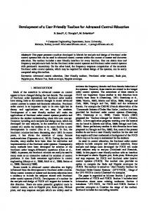
together (the split id is also depicted in Figure 3.4 on page 34, displaying bonds and atoms. The bond relation is symmetric since it resides between two atoms.). In case of the Alzheimer datasets, which have asymmetric relationships, this kind of processing is not a good idea. In Figure 2.7 one can see that a decision tree learner working with the data produced by RELAGGS performs below 50%, if a symmetric representation is chosen. For a correct representation of asymmetric relations, new distinct functors are defined for each argument position: less toxic(a1, b1) then becomes less toxic(less toxic0(a1), less toxic1(b1)) .

One property of Prolog, the possible different arity of functors, has not been tackled so far. it would be possible to fill the missing arguments with “NULL”, but determining the alignment between the two functors is not a trivial task. Another solution would be the introduction of new functors, consisting of the name and the arity as suffix, e.g. a/2 and a/3 would then become a 2 and a 3 . Proper assumes right now that functors of the

same name have the same number of arguments and discards others that differ in their arity. In case that there are different arities present in the data, Proper retains the arity with the most instances and ignores the rest. 11

100

90

80

Accuracy in %

70

60

50

RELAGGS

40

30

20

10

0 alzheimer_toxic-1-firstarg

alzheimer_toxic-2-symmetric

alzheimer_toxic-3-asymmetric

Datasets

Figure 2.7: Different settings for Alzheimer/less toxic: first argument as key, two keys symmetric, two keys asymmetric.

CSV The import of CSV files is pretty straightforward, since the data is already in a column-like representation. If the file contains a header row with the names of the columns, then these are used, otherwise a name is constructed out of the filename and the position of the column. By default the ‘ " ’ is the text qualifier and “ , ” is the column separator, but they can be set to any value. During the import characters that are not “visible” ASCII characters (i.e. byte values from 32–127) are filtered to avoid problems during the aggregation process. A transformation to Unicode1 , like UTF-8 or UTF-16, is preferable, but that would involve major changes. Due to this filtering some information might get lost during the import on other datasets than used in this thesis.

2.2 Propositionalization and Conversion into Multi-Instance Data There are currently three algorithms available for propositionalization and creating multiinstance data in the Proper framework, which can be used for experiments: - RELAGGS - Joiner - REMILK Each of them will be discussed subsequently, how each of them functions and what possible drawbacks there are. 1

Unicode is the attempt to create a universal character encoding scheme for written characters and text. More information about Unicode can be found at http://www.unicode.org/.

12

2.2.1

RELAGGS

The first algorithm we want to discuss is RELAGGS, a database-oriented approach based on aggregations (RELational AGGregationS). The version that was integrated is based on what was used for the comparative evaluation in [Krogel et al., 2003]. These aggregations are performed on the adjacent tables around the table that contains the target attribute, i.e. for each row in the target table it performs for numeric columns both ANSI SQL [Digital Equipment Corporation, Maynard, Massachusetts, 1992] group functions like average, minimum, maximum and sum, as well as non-standard functions like standard deviation, quartile and range. For nominal columns it counts the number of occurences of each value and creates a new column for each value to store the counts. Besides these aggregations based on a single attribute (i.e. the primary key of the target table), it additionally calculates them on pairs of attributes. There, the other attribute has to be nominal, which serves as an additional GROUP BY condition [Krogel & Wrobel, 2003] besides the primary key. RELAGGS uses the names of the primary keys to determine the relations in the database (a drawback of the MySQL2 MyISAM table type used in RELAGGS; even though separate definitions of foreign key relations would be possible with the InnoDB type, the JDBCdriver did not support this at that time).

Modifications From preliminary experiments with the original RELAGGS implementation the following modifications were introduced to relax the constraints RELAGGS imposes on its input data:

- Preflattening. Since the specified version of RELAGGS only aggregates directly adjacent tables, Proper pre-flattens an arbitrarily nested structure. In other words: it flattens all the branches of the tree structure into single tables, which represents a suitable representation for RELAGGS. This is depicted in Figure 2.1, moving from relational data to partially flattened data). - Table hiding. The creation of temporary tables out of the branches (“preflattening”) means that one has to hide the original tables from RELAGGS. Otherwise some data would be aggregated twice, since RELAGGS performs aggregation on all tables that are in relation to the target table. Therefore RELAGGS contains now a black list with 2

MySQL is freely available from http://www.mysql.com/.

13

tables to ignore, containing temporary tables and such that were created by other propositionalization algorithms. - Primary Key restriction. RELAGGS expects an integer as the primary key of a table, which may not always be the case. In some domains, e.g. chemical domains like the Mutagenesis dataset, the primary key of a table is an alpha-numeric string instead. If Proper encounters a non-integer key it automatically generates an additional table with the relation between the original primary key and a new integer key, which is then used in the tables. - Use of Indices. Determining the relation between two tables based on the primary key alone proved to be problematic with the Mutagenesis dataset, where the relation between the different tables (Prolog ground facts) is based on the compound ID. In case of benzene rings it is possible that there exist several rings in one compound and therefore having the same ID, which makes it necessary to relax the restriction from primary keys to indices. - Loss of data. Using ambiguous indices instead of primary keys unfortunately had other consequences as well: posing a query to the database with an aggregation function on an ambiguous index instead of a primary key (using the GROUP BY clause) returns only as many rows as there are unqiue values in the index. The outcome is an aggregated table with (possibly) fewer rows than the target table. To counteract this, Proper always adds an additional column in the table during the import of the data that acts as a primary key. For such ambiguous datasets it is now possible to signalize RELAGGS to either use a specific primary key or the previously mentioned auto-generated one as an additional column in the GROUP BY clause. This problem of data loss arises only due to the fact that MySQL is less strict on the GROUP BY conditions, i.e. that not all columns that appear in the SELECT clause have to appear either in aggregate functions or in the GROUP BY clause (the columns of the target table are only listed in the SELECT clause). A behavior that is not allowed in ANSI SQL, e.g. as implemented in PostgreSQL3 . - Join type. Due to the closed-world-assumption in Prolog data, tables will not necessarily contain full explicit information about the absence of features. In order not to loose any information during aggregation NATURAL JOIN was replaced by LEFT 3

PostgreSQL is freely available from http://www.postgresql.org/.

14

OUTER JOIN . Otherwise the aggregation process could produce an empty result ta-

ble in the worst case. - Column name ambiguity. The previously sketched behavior for nominal columns, namely introducing count-columns for each distinct value of such a column, is not robust concerning generating names for columns. Since MySQL does not allow e.g. “-” or “.” in the name of a column the names are transformed, i.e. the invalid characters are changed into underscores. But here ambiguities can be produced, if one has nominal values like “value-” and “value.”. They are both transformed into “value ”, which results in duplicate column names. To resolve this issue the name is now checked against a hashset whether the same name was already used. If this is the case underscores are then appended to the name as long as necessary to make it unique. The underlying version of the framework for this thesis, i.e. version 0.1.0, supports only MySQL and is not ANSI SQL compatible4 . The computation of the standard deviation for instance is not part of the ANSI SQL Standard, but a handy extension by MySQL. MySQL uses the standard deviation for populations (cf. Equation 2.1) and not the one for samples (cf. Equation 2.2). r P P n x2 − ( x)2 S= n2

(2.1)

s P P n x2 − ( x)2 S= n(n − 1)

(2.2)

Both equations can be rewritten as SQL statements to make them ANSI compliant. Equation (2.1) then becomes SELECT sqrt((count(x)*(sum(x*x)) - (sum(x) * sum(x))) / (count(x) * (count(x)))) FROM

table

and (2.2) can be written as SELECT sqrt((count(x)*(sum(x*x)) - (sum(x) * sum(x))) / (count(x) * (count(x) - 1))) FROM

table

where table is the table the SELECT is performed on and x is the column to retrieve the standard deviation from. There is only one problem with these statements: in case that there are no columns to work on, COUNT returns 0 and therefore raises a Division by zero Exception. 4

Version 0.1.1 moved towards ANSI SQL, additionally supporting PostgreSQL.

15

This “standardization” is necessary for better portability, since different Database systems either do not offer the computation of the standard deviation or calculate it differently. The latter happens in case of PostgreSQL, which calculates the sample and not the population standard deviation. Due to different implementations results might not be comparable.

2.2.2

Joiner

The central processing algorithm in Proper is the Joiner. Like one can see in Figure 2.1 it performs the flattening of the arbitrarily nested structure of the relational data into fitting structures for RELAGGS (maximum depth of 1) and multi-instance learners (one flat table). The Joiner works in a depth-first manner on tree structures, i.e. with a central table where all the others are branching off from. It performs joins starting with the leaves until a branch is completely flattened (for RELAGGS this process is stopped one level above the central table, the root node). To build up this structure the Joiner can either use the auto-discovery of the relations between the tables or user-defined relations (how this can be done is discussed in Section 2.4.1). In order to keep the IO operations to a minimum, the joins are ordered in such a way that the small tables are joined first and the largest last. For RELAGGS a future optimization, mentioned by [Krogel et al., 2003], could be implemented: the propagation of the keys of the tables that are not directly adjacent to the target table5 . Instead of executing expensive joins of whole tables only the necessary key columns would be added to the new table. But since it might not be possible to change the design of an existing database (i.e. a production system with accompanied business logic that depends heavily on the current design) and the complete joins are necessary for MILK and REMILK, these expensive joins were preferred. The LEFT OUTER join is chosen as join operation in order not to loose any information (like mentioned in Section 2.2.1 under Modifications/Loss of data). Since classifiers can handle missing values, the created “NULL” values can be interpreted as missing values. The columns over which the join is performed are simply the intersection of the indices of the first table with all the columns of the second one. In case of the East-West-Challenge in Figure 2.5 with the two tables car and load there is only one index in the car table, the car id . The intersection is then of course car id . If it makes sense for some columns to set the introduced “NULL” values to a specific value (e.g. replacing them with “0”) then this can also be defined and the columns are updated 5

An optional feature implemented in Proper starting with version 0.1.1.

16

after the join. In case that there are duplicate columns beside the join columns, e.g. due to an asymmetric relationship like in the Alzheimer datasets, the second column of such a conflict pair is prefixed with mX , where X is a unique number for the current join. Without doing this one would loose a complete branch of data in asymmetric relationships. To illustrate the functioning of the Joiner we go back to our East-West-Challenge example in Figure 2.5. For RELAGGS one joins until one has only leaves as children of the target table, which can be seen in Figure 2.8. There is only one child, since the East-West-Challenge has only a branching factor of 1.

Figure 2.8: East-West-Challenge joined for RELAGGS.

The complete flattening of the database, which is necessary for a multi-instance learner, is shown in Figure 2.9.

Figure 2.9: East-West-Challenge joined for MI learner.

2.2.3

REMILK

Apart from RELAGGS for creating propositional data and the Joiner for creating multiinstance data, the framework contains a third algorithm called REMILK (RElational aggregation enrichment for MILK6 , the Multi-Instance Learning Kit). REMILK enriches the data the Joiner provided for the multi-instance learner by adding the aggregated data 6

MILK is freely available from http://www.cs.waikato.ac.nz/ml/milk/.

17

produced by RELAGGS to the multi-instance data. This is done via a join of the tables generated by RELAGGS and the Joiner, where the columns from RELAGGS are tagged with a relaggs and the ones from the Joiner with b milk (with this prefixing and a sorted export to an ARFF file the RELAGGS attributes are presented first to the classifier). The resulting table is once again suitable input for a multi-instance learner.

2.3 Export The last step before the classifiers are built and evaluated, is the export. Here the generated tables are transferred to ARFF files to make them available for the WEKA workbench or for MILK. It is possible to exclude certain columns or patterns of columns from being exported, if they contain implicit knowledge like primary keys of tables (and their aggregates) and also to sort them by name for convenience. In case of multi-instance data a bag identifier can be specified explicitly or Proper tries to determine one, based on a heuristic. The heuristic is quite simple: if there is only one index in the table, then this is used, otherwise the first index that does not end with

id . If it ends with

id it is assumed that it was once

the primary key of a table. Allowing this, one could get the primary key of the target table, which might not be the bag ID. This would happen in case of the Mutagenesis dataset, where the compound ID is the key for the relations, but due to ambiguity an additional column has to function as primary key. By skipping indices that look like a primary key Proper can determine the correct bag ID for the Mutagenesis dataset. “NULL” values that were already in the data or introduced during left outer joins are exported as missing values. If the ARFF file would become too large it is also possible to export a stratified sample. Finally WEKA filters can be applied to the data before it is written to the ARFF file, e.g. for transforming all the nominal attributes into binary ones.

2.4 Tools The Proper Toolbox contains already a variety of experiments on example datasets, but it also enables the user to create new ones. In the following several tools will be presented that aid the user in creating new experiments. 18

2.4.1

Relations

For exploring the relations in an existing database one can use the tool Relations, shown in Figure 2.10. With this tool the user can connect to a SQL database server, select a database and create a relation tree starting with the table that contains the target attribute. On each node of the tree only those tables are shown that have a relation to the current node, which makes it very easy to build up a tree. On the other hand, instead of creating the tree by hand, the user can use the auto-discovery of the relations by specifying the maximum search depth. But this latter method is only suitable for databases that were imported from a relational Prolog database or if the branching factor is not too high. Otherwise the tree will get too big to handle.

Figure 2.10: Relations - tool for exploring the relations in a database. Here a user defined tree is displayed for an Alzheimer dataset. With the max. Depth option the user can let Proper suggest a relation tree that can be edited afterwards.

The built tree can then be used in the Propositionalization tools, e.g. RELAGGS, instead of discovering the relations automatically. This is useful if only a few tables should be used in the transformation process. For the East-West-Challenge this tree is given in Figure 2.11. The number in parentheses depicts the number of records in this table, which forms an ordering used during the process of joining tables as already mentioned in Section 2.2.2. train_(20)[train_list1_(63)[c_(63)[l_(63)]]]

Figure 2.11: Relation tree for the East-West-Challenge, where c represents a car and l the corresponding load .

19

2.4.2

Experiments

All experiments that are shipped with the Toolbox are defined in ANT7 files and therefore XML8 . Even though XML is human readable it is still cumbersome to create new experiments from scratch by hand (Figure 2.12 shows a snippet of an ANT file). Even though all tools in Proper provide a command line help, it is still easier to do this with the Builder user interface. ... ... ...

Figure 2.12: Excerpt of an ANT file generated with the Builder (the “...” denotes omissions).

With this front-end the user can define properties of the experiment, like name of the project or the database, as well as what kind of files to import (Prolog or CSV) and how to propositionalize. The above mentioned Relations tool is also part of the Builder (for a screenshot see page 94), which makes it easy to determine what tables should be propositionalized. The Builder is not only able to create ANT files that are executable, but also to open them again for modifications. In order to run the experiments the user can either run them directly from the command line with ANT or use the Run GUI component (cf. Appendix B.1 page 94 for a screenshot). Either experiments created by the Builder or the default ANT files of the Proper Toolbox can be executed here. After loading an ANT file one can choose which target to execute, where the output of the experiments is redirected to the GUI. In case of an unsuccessful execution a dialog pops up 7

ANT is the “make” for Java. The user can define different targets just like in Makefiles, but dependencies have to be stated explicitly, which increases the readability. 8 XML is a simplified version of SGML (ISO 8879), the Standard Generalized Markup Language used for information processing. Further information can be found at the World Wide Web Consortium, http://www.w3.org/XML/.

20

Figure 2.13: Builder - enables the user to build arbitrary experiments.

and lists the erroneous targets. Builder and Run can be used in turn to set up a new experiment: changing parameters with Builder and then testing them with Run. Appendix B.2 contains a guided example of how to use these tools with the East-West-Challenge dataset.

2.4.3

Viewing ARFF files

Another handy tool is the ArffViewer (see Figure 2.14). It displays the content of an ARFF file in tabular form, which enhances the readability significantly. Each column contains the name of the attribute and its type in the header. The class attribute is highlighted in bold font. Despite the name of the tool one can also edit files with it, i.e. changing values of an instance, deleting instances or attributes, sorting the instances based on an attribute. It is also possible to set missing values to a new definite value or to change one specific value of an attribute to another one. For nominal values the ArffViewer provides a dropdown list with all the possible values. It therefore presents an easy way of creating modified copies of a dataset.

2.4.4

Distributed Experiments

Architecture When performing the first experiments with Proper it became clear that the sequential execution of steps on a single machine would be far too slow. Instead of having one ANT file with all the experiments that are executed one after the other it is also possible to use 21

Figure 2.14: ArffViewer - for viewing and editing ARFF files.

a Client-Server-System for running these Java calls (later on only referred to as “jobs”). In Figure 2.15 a general overview is given: a central JobServer manages the jobs and sends them to JobClients that are available for execution. The current system is using a multithreading approach where server and client communicate via XML messages. As soon as a message is received a thread is instantiated that handles the request from then on, the application is immediately going back into listen-mode, waiting for the next request. This approach ensures that no timeouts happen and no messages have to be re-sent due to failure.

Figure 2.15: Basic overview of the Client-Server-Architecture.

Even though the class diagrams in Appendix A.2 on page 85 show both the JobServer and the JobClient as Server-Classes, only the JobServer acts as such. This design originates in the fact that both, the server and the client, are listening for messages and in order to process them efficiently they use multi-threading. It is necessary for the client to accept other messages while processing a job, since the server is checking in regular intervals 22

whether the clients are still alive by sending IsAlive -Messages. If the client is not responding anymore then the server knows that someting went wrong with that client, e.g. an OutOfMemory-Exception or a System-Failure, and can remove it from the list of active clients. With a non-multi-threading client the server would wait forever for such a client. A timeout approach is also not suitable here, since some experiments may take days to complete, depending on the amount of data and the type of classifier being used, and a fixed timeout value would make the server discard a still running client. For managing the clients the server is maintaining two ClientLists (cf. page 85): one with idle clients ( clients ) and another one with clients that are currently processing a job ( pending ). Since a ClientList can also contain a job, we can record which jobs succeeded, failed, are still being processed, or yet to do. Failed jobs can be easily re-run, using this log as input for the JobServer again.

Figure 2.16: Example run of the distributed experiments.

In Figure 2.16 the sequence of actions taking place during a run is depicted. First the user starts the JobServer, which loads the jobs into its queue. After that the JobClient is started, registering itself with the server. At regular intervals the JobDistributor (a special purpose thread of the JobServer) tries to distribute jobs to idle clients. Before the job is sent to the client, it is added to the pending list. As soon as the client receives the job it instantiates a JobClientProcessor object that executes the job and the client goes 23

back to listen mode, while the other thread processes the job. After finishing the execution, either successfully or not, the generated output is sent back to the server and stored there in a global log file. Then the job is removed from the pending list. Once no more jobs are awaiting execution and also all pending ones finished, the server sends a shutdown message to all clients before terminating itself. The messages that are sent between the server and the clients are based on XML, since this poses the most flexible way. The Appendix A.2 (on page 87) shows the different class diagrams and Table 2.1 states the DTD of these messages with a corresponding example. Type Message

DTD
DataMessage

...

FileMessage

...
body data filename line

...
body job status job additional

JobMessage

message head from ip port typ body

(head, body)> (from, type)> (ip, port)> (#PCDATA)> (#PCDATA)> (#PCDATA)> (#PCDATA)>

(data)> (filename, line*)> (#PCDATA)> (#PCDATA)>

(job)> (status, run, additional)> (#PCDATA)> (#PCDATA)> (run*)>

Example Message 192.168.0.1 31415 register ... MIWrapper with base classifier: J48 pruned tree --------------- ... ... eastwest.arff @relation eastwest-Proper 0.1.0 ... ... failed proper.app.Experimenter -class... ...

Table 2.1: DTDs and examples of messages sent between JobServer and JobClient(s).

It is obvious that not all kinds of jobs are parallelizable, that for certain types the ordering is important, e.g. the import of the data has to be finished before the propositionalization takes place. To ensure the order of execution, it is possible to insert so-called synchronization pseudo-jobs. The effect of such a pseudo-job is that the JobDistributor waits until all pending jobs are completed before new jobs are sent to the clients again (see Figure 2.17, “Simple” scheme). An extension to this simple scheme is that dependencies for jobs can be defined: for jobs that depend on each other one puts them in a list in the order they need to be executed, e.g. import before relaggs . If jobs are independent then the list contains only one element.

The result is a number of dependency lists like shown in Figure 2.17. The pending list is now no more a sequential list, but for each dependency list there exists a corresponding slot 24

Simple import: alzheimer import: eastwest synchronize relaggs: alzheimer relaggs: eastwest synchronize export: alzheimer export: eastwest synchronize evaluate: alzheimer evaluate: eastwest evaluate: musk1 ...

Extended alzheimer: import -> relaggs -> export -> evaluate eastwest: import -> relaggs -> export -> evaluate musk1: evalute ...

Figure 2.17: Simple and extended synchronization scheme.

for taking in a job. Figure 2.18 displays these lists. The functionality is best referred to as a “dripping apparatus” where the single “drops” resemble the jobs and the next “drop” can only fall if there is no other “drop” occupying the slot. The server now checks in regular intervals whether there are any free slots and still “drops” available. If that is the case the next “drop” falls into place, i.e. a new job is sent to a free machine for execution. This way of parallelizing jobs guarantees better efficiency, since all jobs that can be distributed will actually be distributed.

Figure 2.18: Visualization of the extended synchronization scheme as “dripping apparatus”.

25

Generating Jobs The current format of the input for the JobServer is just a plain text file where each line contains the class name to execute and the corresponding parameters, in short, like invoking the class from the command line. The Jobber represents a convenient way to extract these calls from existing ANT files (either the default ANT files or ones created with the Builder) to create such a jobfile. In the GUI (cf. Figure 2.19) one can load the specific ANT files to create jobs from. The user can then decide which targets to run in which order and also insert synchronization points where necessary. Sometimes it is necessary to override the properties given in the ANT files with other values, e.g. if a different classifier is to be used and the output should be saved in a different directory, then this can be done on the Properties tab. The current configuration for generating the jobs can be saved in an XML file and if it is reopened then all the necessary ANT files are loaded automatically. Finally the generated jobfile can be edited in the user interface, if necessary (deleting jobs, changing parameters).

Figure 2.19: Screenshot of the Jobber front-end.

Execution The execution of the experiments is pretty straightforward: starting the server with the previously generated jobfile and then subsequently starting the clients. With Unix derivatives it is possible to automate the start up of the clients by using SSH agent9 . The SSH agent provides a passwordless login on remote machines, which is very useful if one has to do 9

Documentation on the SSH agent can be found at http://mah.everybody.org/docs/ssh.

26

many logins. For that reason a few shell scripts were implemented that can start and stop clients that are listed in a plain text file. The scripts perform the following steps for each host listed in that file: - connect to host via ssh - starting a “niced” JobClient with nohup in order to keep it running after logging out again The JobMonitor (cf. page 95 in Appendix B.1) provides a GUI front-end for the command line based JobServer and JobClients. With this tool it is possible to read the job queue of the JobServer, delete certain jobs, shutdown the server or clients. It is also possible to add new jobs to the queue, e.g. ones that failed and have to be re-run.

Figure 2.20: Interaction of the JobMonitor with the JobServer and JobClients.

After the execution the generated logfiles can be processed with other scripts that generate CSV files and LATEX-tables. The CSV files can be further processed by Microsoft Excel templates mentioned in the appendix on page 120.

27

Chapter 3 Related Work

The approaches to propositionalization or generation of multi-instance shown so far are just a tiny fraction of the algorithms available. In this section a few more will be presented and discussed whether they can be integrated in the Proper framework, if this did not already happen.

3.1 MIWrapper The multi-instance learner MIWrapper used throughout the experiments is not a specialpurpose algorithm, but a meta-scheme for multi-instance learning. It is a wrapper around standard propositional learner as described in [Frank & Xu, 2003]. A sketch of the algorithm as outlined in the mentioned paper will be presented and an example where this approach should have an advantage over the aggregations generated by RELAGGS. In multi-instance learning each example is a bag of instances, but only the bag has a class label. The MIWrapper approach assigns each instance of the n instances in the bag a weight proportional to 1/n. By weighting each instance one gets a learner that is not biased to certain examples (ones with more instances), since all the bags have the same weight regardless of the number of instances they contain. For predicting a bag label every instance is run through the built model to obtain the class probability. The average of these probabilities is taken to determine the class label, since all instances are assumed to be equally weighted. The advantage of this approach in contrast to RELAGGS becomes obvious if the data looks like in Figure 3.1. Here are two classes that are basically mirror images of each other, resulting in the aggregates to cancel out each other. The MIWrapper on the other hand is able to derive a useful decision tree from the data, as can be seen in Table 3.1. 29

Figure 3.1: Artificial Dataset. MIWrapper x < 0 | y < 0 : pos (4/0) | y >= 0 : neg (4/0) x >= 0 | y < 0 : neg (4/0) | y >= 0 : pos (4/0)

RELAGGS

:

neg (4/2)

Table 3.1: Unpruned decision trees for the artificial dataset, containing 4 bags with 4 instances each.

3.2 RSD In contrast to the database-oriented approach written in Java, RSD (Relational Subgroup ˇ Discovery) by Filip Zelezn´ y is implemented in Yap Prolog1 . A short introduction will be ˇ given on how RSD works, based on [Zelezn´ y et al., 2003]. RSD takes an inductive Prolog database as input plus an additional mode-language definition. The constraints given with the mode-language define not only the language of subgroup descriptions, but also enable a more efficient induction and focus the search for patterns (thus avoiding the combinatorial explosion mentioned in Section 1.1). 1. Identify features. Here all first-order conjunctions are identified that form a legal feature definition, i.e. they are composed of one or more structural predicates introducing a new variable and of utility predicates that consume all new variables. These features do not contain any constants and can be constructed independently of the input data. An example for a structural predicate is :-modeb(1,hasCar(+train,-car)), where the modeb denotes that the binary predicate hasCar may be used in the body of the clause. The “1” is the maximum number of cars the feature can address of a given train. ‘+’ stands for an input and ‘-’ for an output variable. 1

RSD is freely available from http://labe.felk.cvut.cz/∼zelezny/rsd. A link for Yap Prolog is also provided there.

30

2. Employ constants. In this step the set of features is extended by variable instantiations, where several copies of each feature are instantiated with different constants. Irrelevant features are detected and removed. 3. Produce relational table. The rule induction algorithm, a modified CN2 [Clark & Nibbet, 1989], takes these generated features as input. After creating an appropriate set of features it is possible to generate a single relational table representing the original data. Output for propositional learners can be produced (e.g. for WEKA). Due to the constraints that need to be specified, RSD is currently not integrated into the framework. Still, the generated tables could be post-processed in Proper. By enabling the user to define constraints, the integration could be tighter: the tables in the database could be exported together with the contraints and fed into a Prolog engine that then runs the RSD engine. The output could again be post-processed and used further in Proper.

3.3 SINUS The SINUS2 system developed by Simon Rawles is also Prolog-based and was originally based on LINUS the transformational ILP learner by Lavraˇc and Dˇzeroski (cf. [Lavraˇc & Dˇzeroski, 1994]). The following outline of the propositionalization process is taken from [Krogel et al., 2003] and limited to the steps that are of interest here. The reader may refer to the previously mentioned paper for more information. - Input declarations. SINUS needs the declaration of all the predicates used for ground facts and background knowledge, the cardinality of the relationships between the predicates and the arguments of the predicates. The relation train-car is defined like this:

train2car 2 1:train *:#car * cwa . Here “1” and “*” denotes the

cardinality (“one-to-many”), “#” defines an output argument (otherwise it is an input argument) and since there are two arguments, train and car , this is denoted by “2”. “* cwa” is only of historical relevance (used in the PRD files used in LINUS to define the hypotheses language). - Feature generation. First-order features are constructed recursively, which function as input to the propositional learner. 2

SINUS is freely available from http://www.cs.bris.ac.uk/home/rawles/sinus/.

31

- Feature reduction. Irrelevant and low quality features, according to a quality measure, are removed. - Propositionalization. A table containing the propositional data is constructed and can then be output to a file on which a propositional learner may work. From this brief sketch it is easy to see that SINUS is relatively easy to integrate into the framework. There are basically three steps: the first is to export the relational data to a fitting input format, where each table represents a predicate. The cardinality of the relationships can be easily determined by counting and comparing the keys of tables that are related. Secondly a Prolog engine is invoked to run SINUS with the given data and then to output the propositional data. Finally the output from SINUS could be post-processed in the framework again.

3.4 Stochastic Discrimination Another approach to propositionalization is based on stochastic discrimination as developed by [Kleinberg, 2003]. The application to Machine Learning given in [Pfahringer & Holmes, 2003] will be outlined shortly here. In stochastic discrimination normally thousands of features are generated almost at random and then during prediction the class with the highest vote over all examples (by using equal-vote) is predicted. The features are only generated almost at random since only features that cover more examples than the default percentage for the class are used. But to achieve a good generalization it has also to be ensured that each training example of a class is covered by about the same number of features, even though this may not always be possible in practice.

Figure 3.2: Chemical fragment C-C=C

This method can be used for generating propositional features from structural data, e.g. chemical domains like mutagenicity or carcinogenicity, where we have labeled graphs. But instead of generating random sub-graphs the search is guided by focus examples (an idea borrowed from Progol [Muggleton, 1995]), i.e. to extend a feature only literals which are 32

true for this focus example are used. For each class a user defined number of examples are chosen with a coverage that is below average. A randomized list of all the edges of the graph is generated in such a manner that all but the first entry are connected to at least one prior entry in the list. Every prefix of this list is therefore a connected sub-graph of the example. Finally every sub-graph is either checked whether it appears in every graph or the number of unique instances of the sub-graph in each graph is counted. According to the result of the previously mentioned paper, the latter setting produces better results. Stochastic discrimination could be integrated into the Proper framework, since it is theoretically possible to decompose the sub-graphs into SQL statements and pose these queries to the database. The user only has to define relations between tables that are relevant for discovery, e.g. the atom-bond-atom relation. From this relation-fragment it is possible to generate graphs that can be represented as SQL statements. E.g. the fragment in Figure 3.2 could be written as the statement in Figure 3.3, which is depicted in Figure 3.4. But even though the search in the database could be optimized by introducing indices, there is still a huge number of join operations necessary, which makes it infeasible for longer or more branched fragments. select count(distinct a1.atom id) from atom a1, atom a2, atom a3, atom a4, bond b1, bond b2, bond b3, bond b4 where a1.atom type = ’c’ and a1.bondid = b1.bond id and

b1.bond type = ’-’ and b1.split id = b2.split id

and and

a2.atom type = ’c’ a3.atom id = a2.atom id and a2.bond id = b2.bondid and a3.bond id = b3.bond id

and

b3.bond type = ’=’ and b3.split id = b4.split id

and and

a4.atom type = ’c’ a4.bond id = b4.bond id

Figure 3.3: Chemical fragment as SQL query.

33

Figure 3.4: Graphical representation of the SQL query - the bond predicate is split into two, since it contains two atoms (the split id identifies the entries that belong together). The grey boxes depict the building blocks for longer and branched fragments

34

Chapter 4 Experiments

This chapter will show the feasibility of the presented approach to propositionalization and generation of multi-instance data.1 For this purpose several well-known benchmark datasets will be used. First the different datasets will be introduced and what kind of settings are used for the experiments. Afterwards the results will be presented and discussed in detail.

4.1 Datasets and Settings For the experiments the following well-known benchmark datasets2 were used (the particular names of the datasets used in the tables and figures are also mentioned): - Alzheimer’s disease. These are actually four related problems trying to predict low toxicity, high acetocholinesterase inhibition, good reversal of scopolamine induced deficiency, and inhibit amine re-uptake:

3

alzheimer toxic, alzheimer choline, alzheimer scopolamine, alzheimer amine uptake - Drug-data design. These are the well-known pyrimidine and triazine datasets, examples of the so-called Qualitative Structure Activity Relationship (QSAR) approach to the prediction of drug properties:

3

dd pyrimidines, dd triazines - East-West-Challenge. The well-known trains dataset: eastwest - Genes. From the original KDD Cup 2001 data four datasets were created: one for predicting the function of a gene (without the localization information), another one 1 2

For the experiments version 0.1.0 of the framework was used. The web resources for the datasets can be found in Appendix C.

35

with the localization of a gene as class. From these two non-binary datasets two binarized versions were created (cf. [Krogel et al., 2003]): whether a gene is responsible for a protein that is responsible for “cell growth, cell division and DNA synthesis” is one, and the other one whether the localization of the produced gene is the nucleus or not: genes growth, genes growth bin, genes nucleus, genes nucleus bin - Musk 1/2. Instead of using one flattened table, a target table, containing only the bagID and the class, and a data table, containing the rest of the attributes, were extracted: musk1 rel, musk2 rel - Mutagenesis. Three different approaches were used to turn the mutagenesis data into a multi-instance representation: bags either contain a) all atoms of a compound, or b) all atom-bond tuples of a compound, or c) all adjacent pairs of bounds of a compound: mutagenesis3 atoms, mutagenesis3 bonds, mutagenesis3 chains - Secondary structure of proteins. The task is to predict whether a position in a protein is in an alpha-helix or not:

3

proteins - Suramin analogues. Based on the atomic structure and bond relationships the task is to predict a compound being active or inactive as anti-cancer agent: suramin - Thrombosis. The thrombosis prediction task from the PKDD2001 Discovery Challenge: thrombosis After importing the datasets and generating propositional and multi-instance data from the relational model, one gets the figures shown in Table 4.1. There one finds a detailed overview about the number of classes, the number of attributes that were produced (including the class attribute and in case of multi-instance the bag attribute), the number of records in the result table and how many instances and bags respectively this represents. Since the number of attributes varies depending on the type of post-processing, the outcome of the different settings, one with and the other ones without post-processing, are given. 3

Note: The data generated by the Joiner is actually propositional and not multi-instance in these cases (see Table 4.1).

36

Dataset alzheimer amine uptake alzheimer choline alzheimer scopolamine alzheimer toxic dd pyrimidines dd triazines eastwest genes growth genes growth bin genes nucleus genes nucleus bin musk1 rel musk2 rel mutagenesis3 atoms mutagenesis3 bonds mutagenesis3 chains proteins suramin thrombosis

Classes 2/2/2 2/2/2 2/2/2 2/2/2 2/2/2 2/2/2 2/2/2 13/13/13 2/2/2 15/15/15 2/2/2 2/2/2 2/2/2 2/2/2 2/2/2 2/2/2 2/2/2 2/2/2 4/4/4

Attr. (Sett. 1) 237/62/298 251/70/320 237/60/296 251/70/320 95/90/184 125/118/242 66/26/91 27/49/138 27/49/138 27/49/134 28/49/134 1661/168/1828 1661/168/1828 26/12/37 56/18/73 88/26/113 22/22/43 151/22/172 293/91/394

Attr. (Sett. 2-6) 237/40/276 251/40/290 237/40/276 251/40/290 95/8/102 125/10/134 66/11/76 27/12/40 27/12/40 27/12/40 28/12/40 1661/168/1828 1661/168/1828 26/5/30 56/9/64 88/13/100 22/3/24 151/9/159 293/65/357

Records 686/686/686 1326/1326/1326 642/642/642 886/886/886 1762/1762/1762 23650/23650/23650 20/213/213 4346/14238/14238 4346/14238/14238 4346/14238/14238 4346/14238/14238 92/476/476 102/6598/6598 188/1618/1618 188/3995/3995 188/5349/5349 1612/1612/1612 11/2378/2378 770/86452/86452

Inst./Bags/Bags 686/686/686 1326/1326/1326 642/642/642 886/886/886 1762/1762/1762 23650/23650/23650 20/20/20 4346/4346/4346 4346/4346/4346 4346/4346/4346 4346/4346/4346 92/92/92 102/102/102 188/188/188 188/188/188 188/188/188 1612/1612/1612 11/11/11 770/770/770

Table 4.1: Overview of the produced data, where each column shows the values for RELAGGS/Joiner/REMILK.

Setting 1 2 3 4 5 6

Classifier unpruned REPTree, for genes * LogitBoost/DecisionStump LogitBoost/DecisionStump unpruned REPTree LogitBoost/unpr. REPTree max depth 1 LogitBoost/unpr. REPTree max depth 3 AdaBoostM1/pruned J48

Parameter -P -M 0, for genes *: default default/default -P -M 0 default/-P -M 0 -L 1 default/-P -M 0 -L 3 default/default

Nominal Attributes NominalToTrueBinary -

Missing Values for binarized attr. replaced by “0” -

Table 4.2: Settings for the experiments. In case of multi-instance data the MIWrapper was used with default parameters.

Attribute att a b ?

NominalToBinary att 1 0 0

NominalToTrueBinary att=a att=b 1 0 0 1 0 0

Table 4.3: Different behavior of the original NominalToBinary filter and the modified version, if nominal attribute contains only two distinct values (“att” is the name of the example attribute). Missing values are replaced with “0”.

37

Based on this data several settings of experiments are executed as listed in Table 4.2. All the experiments were run on Intel Pentium 4 machines with 2.60GHz and 512MB of RAM, where the Java Virtual Machine (JVM) was limited to 1.2GB of heap size (missing entries in the tables and figures, denoted by “-” or missing bar, mean that the JVM runs out of memory). The following learning schemes (in alphabetical order) were used: - AdaboostM1. A standard boosting algorithm by [Freund & Schapire, 1996]. - DecisionStump. 1-level decision tree with a binary split and a separate branch for missing values. - J48. The Java implementation of Quinlan’s C4.5 (cf. [Quinlan, 1993]). - LogitBoost. Performs boosting based on additive logistic regression [Friedman et al., 1998]. - REPTree. An unpruned REPTree is a decision tree built with info gain. In all experiments 10 runs of 10-fold stratified cross-validation was used, only on eastwest and suramin Leave-One-Out was employed, due to the small amount of instances or bags respectively. For turning nominal attributes into “binary” ones, a modified version of the NominalToBinary Weka filter was used. This filter creates a new attribute for each distinct value of a nominal attribute, whereas the original filter does this only for nominal attributes that have more than two distinct values, otherwise the attribute is thought to be already binary. Table 4.3 shows the different outcome of the original and the modified filter if they encounter an attribute with only two distinct values. Here one can simulate the closed-world-assumption of imported Prolog data, by setting the missing values to “0”: if a feature is not explicitly mentioned then it is not missing (“NULL”), but not existing (“0”).

38

4.2 Results The following sections discuss the previously introduced experiment settings in detail, the intention of each setting and the outcome.

4.2.1

Setting 1

For a fair comparison (cf. Figure 4.1 and Table 4.4) between the different algorithms an unpruned decision tree was chosen. Not J48, since it still performs some pre-pruning, but REPTree. Pruning was not used, because it is sensitive to the absolute value of each instance’s weight, an effect that makes it harder to provide a fair comparison. For a simulation (at least on single-instance data) of the RELAGGS “count” ( CNT VAL column) of nominal attributes in adjacent tables the NominalToTrueBinary filter was used in combination with replacing all missing values in such binarized columns with “0”. It is only possible to simulate this behavior to a certain degree: no aggregation takes place in the target table and therefore RELAGGS does not perform any binarization there. The filter on the other hand still transforms every nominal attribute. Due to the method of dealing with missing values using fractional instances [Quinlan, 1993], the unpruned decision tree literally “explodes” for data with nominal attributes that contain lots of missing values (because REPTree generates a copy of an instance with a missing value for each branch, and does so simultaneously for each branch). This happened in case of the genes * datasets, where it was not possible to create a tree that fitted into memory. In this case the ensemble LogitBoost/DecisionStump was used, to get any results. Apart from the Alzheimer, the genes nucleus * and the thrombosis datasets, the three approaches perform more or less equal. The difference in case of the Alzheimer single-instance datasets between the RELAGGS and Joiner data is due to missing values, which is discussed in detail in Section 4.3. In Setting 2 a different outcome can be seen for the genes nucleus * datasets. In other experiments, where the attributes were ordered in such a way that first the Joiner ones and then the RELAGGS ones appeared, it was hypothesized that the order affected the learner. Since the order is now reversed, first RELAGGS and then Joiner, and the outcome is still unchanged, this can be ruled out. The differences in the eastwest and the suramin datasets are not of such importance due to the high standard deviation of 40–50% (which holds true for all the following settings).

39

100 90 80

Accuracy in %

70 60 RELAGGS Joiner REMILK

50 40 30 20 10

er _ he im al z

al z

am in e_ up h al ei ta zh m ke ei er m _c er ho _s lin co e po al la zh m in ei e m er dd _t ox _p ic yr im id in dd es _t ri a zi ne s ea st ge w es ne t ge s_ ne gr ow s_ gr th ow th ge _b ne in ge s_ ne nu s_ cl eu nu s cl eu s_ bi m n us k1 _r m el m ut us ag k2 en _r es m el ut is 3_ ag at en om m es ut s is ag 3_ en bo es nd is s 3_ ch ai ns pr ot ei ns su ra m th in ro m bo si s

0

Datasets

Figure 4.1: Comparison for Setting 1.


RELAGGS 87.53 ± 89.05 ± 87.86 ± 92.75 ± 92.41 ± 74.75 ± 80.00 ± 31.69 ± 84.26 ± 76.18 ± 87.20 ± 80.13 ± 72.83 ± 79.58 ± 85.38 ± 85.31 ± 59.52 ± 54.54 ± 96.67 ±

4.04 2.79 4.37 2.90 2.17 0.84 41.03 1.55 0.42 2.09 1.43 15.21 13.44 8.90 7.85 7.83 4.08 52.22 1.45

Joiner 73.53 79.19 73.92 88.56 92.38 74.75 55.00 34.00 84.36 57.22 81.64 76.82 82.72 83.04 83.74 59.52 63.63 87.39

± ± ± ± ± ± ± ± ± ± ± ± ± ± ± ± ± ±

5.26 3.98 4.77 3.53 2.15 0.84 51.04 1.15 0.24 2.32 14.68 12.61 8.24 7.74 7.98 4.08 50.45 2.87

REMILK 87.59 ± 89.04 ± 87.87 ± 92.72 ± 92.41 ± 74.76 ± 75.00 ± 33.47 ± 84.36 ± 62.78 ± 78.54 ± 79.40 ± 74.40 ± 80.46 ± 86.84 ± 85.40 ± 59.50 ± 54.54 ± -

Table 4.4: Accuracy and standard deviation for Setting 1.

40

3.91 2.74 4.32 2.92 2.17 0.84 44.42 1.20 0.37 2.15 1.71 14.54 13.73 9.15 7.11 8.66 3.94 52.22

4.2.2

Setting 2

Setting 2 uses an ensemble consisting of LogitBoost and DecisionStump, both with default settings (i.e. 10 iterations for the boosting algorithm). The results can be found in Figure 4.2 and Table 4.5. In contrast to Setting 1 no post-processing of nominal values took place, since the DecisionStump handles missing values differently. It treats the missing values as another value, whereas decision trees like REPTree treat them as unknown. With this setting there are basically no differences in the result for the different approaches, only on the mutagenesis3 * datasets where the MIWrapper produces worse results. Comparing the results for the genes nucleus * datasets with the ones from the previous setting (binarization of nominal attributes and replacing missing values) now all three approaches perform equally well. This dataset is apparently sensitive to binarization and/or replacing missing values. The thrombosis datatset, in case of the Joiner data, also profits from the different handling of missing values. This dataset contains a lot of missing values, especially in the nominal attributes. By treating these as a separate value, one gets a nearly perfect representation (above 99% and standard deviation of less than 1%). That the combination of the two datasets (REMILK) does not fit into memory is not surprising due to the fact, that the dataset has 357 attributes and 86,452 instances, resulting in a matrix with 30,863,364 cells. musk1 rel is a dataset where the Joiner has a slight advantage compared to the other two approaches, even though this dataset contains no missing values at all. The aggregation apparently loses some important information crucial to the predictive power.

41

100 90 80

Accuracy in %


50 40 30 20 10

er _ he im al z

al z


0

Datasets



RELAGGS 84.46 ± 77.93 ± 73.47 ± 79.90 ± 83.12 ± 66.15 ± 75.00 ± 31.69 ± 84.26 ± 76.18 ± 87.20 ± 77.98 ± 78.56 ± 76.48 ± 84.28 ± 85.21 ± 59.82 ± 54.54 ± 97.38 ±

3.86 3.28 5.40 3.67 2.92 1.14 44.42 1.55 0.42 2.09 1.43 15.10 12.66 9.07 8.36 8.25 3.50 52.22 1.38

Joiner 85.43 76.59 74.83 80.33 83.14 66.27 60.00 32.18 84.13 74.75 86.44 81.67 78.90 67.02 72.87 73.02 60.29 63.63 99.33

± ± ± ± ± ± ± ± ± ± ± ± ± ± ± ± ± ± ±

3.75 3.17 5.18 4.29 2.96 1.72 50.26 1.44 0.51 2.00 1.26 13.83 12.20 3.05 6.80 8.90 3.67 50.45 0.85

REMILK 85.93 ± 76.59 ± 74.26 ± 81.67 ± 83.12 ± 66.27 ± 80.00 ± 31.53 ± 84.34 ± 76.67 ± 87.30 ± 77.30 ± 78.66 ± 76.67 ± 83.93 ± 84.40 ± 59.86 ± 54.54 ± -


42

4.38 3.17 5.33 3.60 2.92 1.72 41.03 1.48 0.58 1.94 1.30 14.93 12.71 9.44 7.31 8.64 2.80 52.22

4.2.3

Setting 3

Like in Setting 1 this setting uses again an unpruned REPTree. But this time no transforming of nominal attributes and no replacing of missing values takes place (cf. Figure 4.3 and Table 4.6). The purpose of this setting is to explore the possible effects of the NominalToTrueBinary filter and the replacing of missing values with “0”. Of course, problems arise from the use of an unpruned decision tree in case of larger datasets, like genes * and thrombosis. Even after removing all the nominal values with a lot of missing values from the genes * the JVM runs out of memory working on the Joiner/REMILK data. The thrombosis dataset with its 80,000+ instances also contains many nominal attributes with a high percentage of missing values, resulting in JVM crashes because of insufficient memory (i.e. JVM heap size). That the single-instance datasets Alzheimer with their limited number of instances (around 1000) do not produce any results for the Joiner data can only be explained with the huge amount of missing values most of the attributes have. Table 4.7 shows what percentage of attributes in a dataset have at least a given percentage of missing values, e.g. in the alzheimer toxic dataset 81.82% of the nominal attributes have a missing value portion of more than 75%. The datasets shown in that table were generated with the Joiner. The suramin dataset also runs out of memory in case of the Joiner data, which is apparently linked to the fact that of the 9 attributes (including the class), 5 have 53% of missing values. Especially one nominal attribute, the atom identifier, has more than 1100 distinct values. A surprising finding is the significant increase for the multi-instance data in the dd triazines dataset (standard deviation is only around 0.5%), whereas dd pyrimidines suffers compared to Setting 1. Since there are no missing values in these datasets, the reason for this must lie in the binarization of the nominal attributes with the NominalToTrueBinary filter.

43

100 90 80

Accuracy in %


50 40 30 20 10

al z

in am su r

te in s pr o

m m us ut k2 ag _r en el es i s m 3_ ut at ag om en s es is m 3_ ut bo ag nd en s es is 3_ ch ai ns

t

k1 _r el

m us

ea st w es

al z

he im

er _

am

in e_ up ta he ke im al er zh _ ch ei m ol er in _s e co po la m al in zh e ei m er _t ox dd ic _p yr im id in es dd _t ri a zi ne s

0

Datasets


Dataset alzheimer amine uptake alzheimer choline alzheimer scopolamine alzheimer toxic dd pyrimidines dd triazines eastwest musk1 rel musk2 rel mutagenesis3 atoms mutagenesis3 bonds mutagenesis3 chains proteins suramin

RELAGGS 87.53 ± 89.05 ± 87.86 ± 92.75 ± 92.41 ± 74.75 ± 80.00 ± 80.13 ± 72.83 ± 79.58 ± 85.38 ± 85.31 ± 59.52 ± 54.54 ±

Joiner 4.04 2.79 4.37 2.90 2.17 0.84 41.03 15.21 13.44 8.90 7.85 7.83 4.08 52.22

86.92 82.20 40.00 81.64 76.82 82.61 83.47 84.17 59.12

± ± ± ± ± ± ± ± ± -

2.25 0.58 50.26 14.68 12.61 8.03 8.11 7.45 5.08

REMILK 86.07 ± 88.66 ± 87.66 ± 91.16 ± 86.92 ± 82.41 ± 70.00 ± 79.40 ± 74.40 ± 80.46 ± 86.90 ± 85.35 ± 59.92 ± 54.54 ±

4.10 2.89 4.47 2.91 2.21 0.57 47.01 14.54 13.73 9.15 7.11 8.62 1.41 52.22


Perc. of missing values in attribute >33% >50% >66% >75%

alzheimer toxic All Nominal 80.00% 90.91% 75.00% 90.91% 75.00% 90.91% 65.00% 81.82%

genes growth All Nominal 22.22% 33.33% 0.00% 0.00% 0.00% 0.00% 0.00% 0.00%

thrombosis All Nominal 59.09% 55.56% 36.36% 22.22% 36.36% 22.22% 36.36% 22.22%

Table 4.7: Overview of portion of attributes with missing values in the alzheimer toxic, genes growth and thrombosis multi-instance datasets (generated with the Joiner). It is checked how many attributes (in percent) have a percentage of missing values above a certain threshold. This is done for All attributes and only for Nominal ones.

44

4.2.4

Setting 4

Setting 4 uses LogitBoost with default parameters like Setting 2, but instead of taking DecisionStump as the other part of the ensemble it uses a decision tree, the REPTree, with a maximum level of 1. Again there was no post-processing of nominal attributes and missing values. The goal of this experiment is to check, whether the different handling of missing values and different treatment of nominal attributes has an impact on the results. REPTree, like already mentioned in Setting 2, treats missing values as unknown, whereas the DecisionStump treats them as a separate value and creates an extra branch for it. Furthermore, the REPTree uses multi-way splits on nominal attributes in contrast to the DecisionStump, which performs binary splits on them. The REPTree runs into memory problems once again, even though not as severe as in the previous setting. Here several genes * datasets generated by REMILK, as well as the thrombosis dataset, would consume more memory than allowed, i.e. 1.2GB. In case of the thrombosis dataset not even the multi-instance data produced by the Joiner succeeded, i.e. building a model and running cross-validation, failed running out of memory. As one can see in Figure 4.4 (and the corresponding Table 4.8), all the Alzheimer datasets perform a little bit less well, as well as genes growth *. On the other hand, the Drug-data datasets, dd pyrimidines and dd triazines, experience a boost in accuracy of over 10%, an indicator that for these datasets the treatment of nominal attributes is quite essential (missing values are of no concern here, since the datasets do not contain any). It also shows that the binarization that RELAGGS performs on nominal attributes is somewhat of a disadvantage when using such a shallow tree. In such cases the un-binarized multi-instance data seems to represent the better approach.

45

100 90 80

Accuracy in %


50 40 30 20 10

er _ he im al z

al z


0

Datasets



RELAGGS 80.85 ± 74.78 ± 71.33 ± 77.66 ± 83.12 ± 66.15 ± 85.00 ± 24.13 ± 83.23 ± 82.39 ± 92.65 ± 77.88 ± 78.26 ± 76.59 ± 84.06 ± 85.10 ± 59.82 ± 54.54 ± 97.46 ±

3.81 3.25 5.66 3.25 2.92 1.14 36.63 1.59 0.67 1.63 1.16 15.20 12.58 9.04 8.37 8.26 3.50 52.22 1.30

Joiner 74.53 71.86 68.45 74.14 95.06 89.15 65.00 24.10 83.23 79.74 92.09 81.90 78.90 67.87 72.87 72.92 59.12 63.63

± ± ± ± ± ± ± ± ± ± ± ± ± ± ± ± ± ± -

4.56 3.22 5.50 3.92 1.61 0.71 48.93 1.61 0.67 1.79 1.03 13.67 12.20 4.11 6.67 8.61 5.08 50.45

REMILK 80.85 ± 74.78 ± 71.33 ± 77.66 ± 95.06 ± 89.15 ± 80.00 ± 92.56 ± 77.87 ± 78.56 ± 76.67 ± 83.82 ± 84.35 ± 60.17 ± 54.54 ± -


46

3.81 3.25 5.66 3.25 1.61 0.71 41.03

1.08 15.24 12.74 9.44 7.26 8.63 1.19 52.22

4.2.5

Setting 5

This Setting uses a logit-boosted REPTree with a maximum level of 3 instead of 1. With this it is possible to explore how important the interactions among attributes are for the different datasets. Since an unpruned REPTree grows quite big in case of nominal attributes with missing values, another preprocessing step was performed for the genes * datasets: all nominal attributes with at least 33% of missing values were removed. For the genes relation relation these were the attributes class , complex and motif . The results of this batch of experiments can be found in Figure 4.5 and Table 4.9. Like in Setting 3, the suramin dataset crashes with an OutOfMemory-Exception. A REPTree with a maximum level of 3 is apparently already to deep to process the multi-valued attributes with many missing values. For the thrombosis dataset only the RELAGGS data works with these settings. In comparison to the REPTree from the previous experiment with just one level, the accuracy of RELAGGS increased significantly (roughly 10%) for the Alzheimer and the Drugdata datasets.

The difference between RELAGGS and Joiner data increases for

alzheimer amine uptake and alzheimer scopolamine, but vanishes for alzheimer choline. The one for alzheimer toxic does not change remarkably. The findings for Alzheimer, regarding the accuracy, are linked directly to the size of the datasets: smaller datasets result in a decrease of accuracy and greater ones in an increase, an indicator for overfitting. In contrast to that, both genes nucleus datasets drop in their accuracy significantly, the increased depth of the tree apparently introduces overfitting. This overfitting also happens to the classifier built on top of the REMILK data for genes growth, since the accuracy for the RELAGGS data is slightly worse and the one for the Joiner data is a little bit better. The expected outcome was that the differences would cancel out each other. The Mutagenesis datasets improve, but not so dramatic in case of RELAGGS. The multiinstance data on the other hand profits more from the increased depth of the tree.

47

100 90 80

Accuracy in %


50 40 30 20 10

er _ he im al z

al z


0

Datasets



RELAGGS 90.15 ± 85.75 ± 86.08 ± 93.28 ± 93.17 ± 73.18 ± 80.00 ± 21.52 ± 83.00 ± 79.00 ± 82.76 ± 81.78 ± 79.00 ± 81.27 ± 88.56 ± 86.38 ± 59.54 ± 54.54 ± 97.58 ±

3.84 3.31 4.92 2.58 1.79 0.91 41.03 1.34 0.64 1.77 1.65 14.51 12.63 8.82 8.02 7.06 3.94 52.22 1.22

Joiner 80.46 86.20 75.34 89.26 92.71 90.31 40.00 27.16 84.04 68.99 77.82 84.65 81.07 79.21 80.85 83.80 59.12

± ± ± ± ± ± ± ± ± ± ± ± ± ± ± ± ± -

4.52 2.79 4.87 3.02 1.87 0.52 50.26 1.19 0.36 2.05 1.99 11.22 11.89 9.29 8.58 7.87 5.08

REMILK 90.39 ± 85.85 ± 85.82 ± 93.25 ± 92.76 ± 90.25 ± 80.00 ± 14.11 ± 82.22 ± 74.63 ± 82.40 ± 80.86 ± 79.96 ± 81.79 ± 88.11 ± 87.38 ± 60.11 ± 54.54 ± -


48

3.33 3.31 4.92 2.75 1.77 0.60 41.03 1.42 1.03 1.81 1.85 14.10 12.71 8.98 7.04 8.21 1.30 52.22

4.2.6

Setting 6

The final experiment setting consists of J48 boosted by AdaBoostM1. This combination was chosen since J48 is a commonly used decision tree learner and boosting provides, in general, better results. The results (cf. Figure 4.6 and Table 4.10) from this setting are also used in discussions of performance regarding tree sizes and runtimes later on in Section 4.4. RELAGGS achieves the best results on the Alzheimer datasets, whereas the MIWrapper performs not as well as in the previous setting. Considering Table 4.11 (in Section 4.4) showing that the average size of trees generated from the RELAGGS data is about one magnitude larger than the ones for the Joiner data this fact is not suprising at all. The combination of both datasets results in a model with an accuracy as good as RELAGGS, but with smaller trees. All three approaches work surprisingly well on the dd pyrimidines dataset. In case of the dd triazines dataset, the JVM crashes with an OutOfMemory-Exception during the execution the 10 runs of the 10-fold cross-validation and not already during building the model. Exceptions happened also to the binarized versions of the genes datasets and the thrombosis dataset, running on the REMILK data. For genes growth the classifier quit on the Joiner data. An interesting result was the increasing accuracy on the genes nucleus dataset from RELAGGS to REMILK, where the combination of RELAGGS and Joiner data produces the best result of the three (the outcome that was hoped for in general). In case of genes growth (RELAGGS/REMILK) the tree is always pruned back to one node, predicting the majority class. The suramin dataset normally produced accuracies around 50%. The best results were always achieved with the Joiner data, but with J48 the RELAGGS data achieves an accuracy of more than 70% (still, the high standard deviation of roughly 50% persists).

49

100 90 80

Accuracy in %


50 40 30 20 10

er _ he im al z

al z


0

Datasets



RELAGGS 92.76 ± 91.18 ± 90.58 ± 96.60 ± 96.81 ± 70.00 ± 35.25 ± 84.19 ± 69.88 ± 93.46 ± 83.76 ± 80.20 ± 79.99 ± 87.83 ± 87.39 ± 59.52 ± 72.72 ± 97.33 ±

3.08 2.34 3.55 1.94 1.33 47.01 0.00 0.71 2.39 1.37 12.60 10.78 7.84 7.13 7.33 3.74 46.70 1.55

Joiner 75.50 79.87 69.22 77.28 95.17 90.90 50.00 82.54 75.52 93.59 87.03 82.20 78.41 82.61 84.76 59.12 63.63 90.35

± ± ± ± ± ± ± ± ± ± ± ± ± ± ± ± ± ±

5.61 3.28 5.28 4.43 1.89 0.67 51.29 1.09 1.94 1.40 11.22 11.58 7.98 6.66 7.68 5.08 50.45 0.91

REMILK 93.15 ± 90.69 ± 91.28 ± 96.76 ± 96.94 ± 80.00 ± 35.25 ± 79.62 ± 82.85 ± 66.71 ± 80.40 ± 88.40 ± 88.34 ± 59.36 ± 72.72 ± -


50

3.30 2.83 4.18 2.17 1.38 41.03 0.10 3.55 13.63 13.85 8.30 6.85 7.44 2.56 46.70

4.3 Comparison of RELAGGS and Joiner During the experiments the following question arose: why does the data produced by RELAGGS for single-instance problems, like the Alzheimer datasets, achieve better results compared to the one created by the Joiner, even though there was no aggregation happening (depicted in Figure 4.7, the bars with the suffix “-1-all”). In the following the necessary steps are outlined to obtain the same results for both approaches. The first step is to remove all the columns created by aggregate functions from the RELAGGS data, leaving only those that are generated by MAX . MAX is still used, since otherwise no data from adjacent tables will be added to the result table. The other reason for MAX is that it does not introduce any new knowledge in case of single-instance data: it either

returns the only value if there is a corresponding row in the adjacent table, or “NULL” if not. MIN can also be used for this purpose instead of MAX , since these functions return the same

value in single-instance data. The data generated by the Joiner is processed in such a way that all nominal values beside the bag ID and the class are transformed to binary attributes with the NominalToTrueBinary filter. Thus simulating the “counting” of RELAGGS (i.e. the CNT VAL column) performed on nominal attributes (in single-instance data the count is either “0” or “1”). But still the results differ as can be seen in Figure 4.7 (results with suffix “-2-no agg”). One difference in the data is still left: the NominalToTrueBinary filter leaves missing values alone, in contrast to RELAGGS that inserts a count of “0” if it cannot find a certain value in an adjacent table. By changing the missing values of binarized attributes in the Joiner data to “0” the same results can be achieved (results with suffix “-3-missing to zero” in Figure 4.7). The conclusion from this comparison is that the absence of a feature is valuable information. Especially in chemical domains a missing functional group can change the mode of functioning of a molecule quite profoundly.

4.4 Tree sizes and runtimes Depending on the goals, the highest accuracy might not always be the best choice. In a time-critical system, where one always has to rebuild models within a given time limit, one will settle with a less accurate, but faster, model. It is better to have a result than none. If one is thinking of embedded systems with their limited system resources, smaller models 51

100 90 80

Accuracy in %

70 60 RELAGGS Joiner

50 40 30 20 10

am

er _

he im

al z

he im

al z

al z

he im

er _

am

in e_ up ta er ke in _a e_ -1 m -a up in ll ta e_ k up e2ta n ke o_ -3 ag -m g is si ng al _t zh o_ ei ze m ro er al _c zh h ei ol al m i ne zh er -1 ei _c -a m ho er ll lin _c eho 2lin n eo_ 3ag m g al is si zh n ei g_ m to e _z r_ al zh sc er ei op o al m ol zh er a ei m _s m i n co er epo _s 1la al co m l po in la em 2 -n in o_ e3ag m g is si ng _t o_ al zh ze ei ro m er al _t zh ox e ic al im -1 zh er -a ei _t ll m ox er i c _t -2 ox -n ic o _a -3 -m gg is si ng _t o_ ze ro

0

Datasets

Figure 4.7: Performance comparison of RELAGGS and Joiner on the Alzheimer dataset (the suffices indicate the step referenced in the text). The used classifier was the tree-classifier J48 with default values.

are preferred over larger (and possibly more accurate) ones. The basis for the discussion is Setting 6 using AdaBoostM1 combined with J48. Only datasets where all three approaches generated results are considered. In the following the size of the trees, the time for building a model and evaluating it, and the performance of different database systems are taken into account. All figures are the average over 10 iterations of AdaBoostM1 (if boosting could be performed at all). In Table 4.11 one can see that RELAGGS is producing the smallest tree 10 out of 14 times (on average). A quite interesting fact is that the REMILK trees only get smaller compared to the RELAGGS trees, if the multi-instance data from the Joiner produces the smallest tree. The expectation that the combination of the multi-instance data with the aggregated data would produce the best results was not fulfilled. Most of the time (9 out of 14) it generated marginally better results than RELAGGS, but with a greater standard deviation. Based on the current results one can say that RELAGGS produces in general the smaller trees, but that seems to be quite dataset dependent (for all Alzheimer datasets, the Joiner approach creates the smallest trees). The results in Table 4.12 suggest that RELAGGS is the fastest approach, considering the overall running time. Even though RELAGGS and the Joiner are both fastest in the same number of cases, the multi-instance learner is only faster in case of single-instance datasets due to the smaller number of attributes it has to consider for building the model. Measured 52

Dataset alzheimer amine uptake alzheimer choline alzheimer scopolamine alzheimer toxic dd pyrimidines dd triazines eastwest genes growth genes growth bin genes nucleus genes nucleus bin musk1 rel musk2 rel mutagenesis3 atoms mutagenesis3 bonds mutagenesis3 chains proteins suramin thrombosis # Times Smallest Tree

RELAGGS 73.60 166.80 95.00 80.80 144.20 4.00 1.00 97.14 327.25 161.90 11.00 9.60 22.20 14.00 13.60 6.56 3.00 19.20 10

Joiner 10.89 16.63 9.00 8.60 391.80 5096.50 31.40 186.80 1317.67 410.70 44.80 182.80 37.57 109.60 183.20 14.33 15.20 600.00 4

REMILK 70.50 136.00 49.90 47.40 178.60 5.00 1.00 1082.25 13.00 31.00 37.00 33.00 35.00 6.56 5.00 1

Table 4.11: Tree size for AdaBoostM1/pruned J48 averaged over 10 iterations (only datasets with results for all three approaches were considered for the “Smallest Tree” count).

absolutely, the multi-instance learner is slower. Finally the performance of different database systems, namely MySQL and PostgreSQL, will be discussed (based on Proper version 0.1.1; performed on a mobile Pentium 4/1.60GHz with 512MB of RAM). Oracle 10g, a commercial product, could not be included due to lack of disk-space. But preliminary tests with the eastwest dataset (Oracle 10g is sort of an overkill for that dataset, since the initial size for a database is more than 500MB) revealed the applicability of the framework. The only drawback was that the databases cannot be created “on the fly” like with MySQL or PostgreSQL, but have to be installed by a database administrator (DBA) beforehand. As one can see in Table 4.13, the version optimized for MySQL (and therefore not portable) performs best. Due to modifications to the RELAGGS code, concerning the adding of columns (in ANSI SQL one can add only one column at a time, whereas in MySQL one can add as many as necessary) and the setting of the default values for numerical columns (PostgreSQL does not yet support the DEFAULT x property, it has to be simulated with a subsequent UPDATE statement), the performance drops significantly. Since PostgreSQL is a fully-fletched object-relational database system, it seems to suffer from this overhead quite dramatically. Given the current results one might want to stick to the optimized MySQL version, if one is not dependent on an ANSI SQL compatible system. MySQL also appears to 53

Dataset alzheimer amine uptake alzheimer choline alzheimer scopolamine alzheimer toxic dd pyrimidines dd triazines eastwest genes growth genes growth bin genes nucleus genes nucleus bin musk1 rel musk2 rel mutagenesis3 atoms mutagenesis3 bonds mutagenesis3 chains proteins suramin thrombosis # Times Fastest

RELAGGS 3408 6409 1687 3096 3613 2 1845 15018 9618 18763 811 1393 37 60 128 435 2 524 6

Joiner 399 1589 491 838 75 1023 4 200679 119363 206016 1240 59538 41 510 1385 3 39 31777 6

REMILK 1880 7932 4888 8745 2874 1 8647 367823 445 54427 288 3106 3964 56 32 2

Table 4.12: Runtimes in seconds for AdaBoostM1/pruned J48 (i.e. time to build the classifier for printing the tree and to execute 10 runs of 10-fold CV). Only datasets with results for all three approaches were considered for the “Fastest” count.

Dataset alzheimer toxic dd triazines eastwest genes nucleus musk2 rel mutagenesis3 chains proteins suramin thrombosis

MySQL (optimized) Imp. REL Joi. 8 30 10 170 96 10 1 1 1 19 6 6 73 53 3 16 3 0 7 3 0 11 4 1 593 col 31

REM 14 21 1 339 220 9 13 6 1478

MySQL Imp. REL 8 222 158 796 3 6 21 12 69 2136 15 7 6 6 9 51 594 col

Joi. 14 11 2 4 4 0 0 1 25

REM 17 11 1 1235 col 13 12 6 -

PostgreSQL Imp. REL 157 359 3475 abrtd 14 11 661 80 401 col 267 21 255 89 -

Joi. 23 abrtd 2 8 9 2 1 -

REM 17 abrtd 1 15 col 5 2 -

Table 4.13: Runtimes in seconds for different database systems (Imp. = Import, REL = RELAGGS, Joi. = Joiner, REM = REMILK). Note: “col” means that too many columns were produced (but not necessarily a program termination), “abort” that the process was aborted, because consuming too much time, and “-” that the process was not executed at all.

54

be more stable compared to PostgreSQL (if that statement is possible, based on the experience with relatively small databases), PostgreSQL e.g. just hung sometimes, without any apparent reason, while importing the alzheimer toxic data.

4.5 Summary Summarizing the above discussed experiments, one can say that even though RELAGGS is not the fastest approach for generating the data used as input for the classifier (the Joiner beats RELAGGS quite often, cf. Table 4.13), the smaller amount of data produced due to the aggregation speaks in favour of RELAGGS. The memory usage for a normal propositional classifier based on RELAGGS data is considerably less than that of MILK, using the data generated by the Joiner or REMILK. This is crucial if one considers larger datasets, like thrombosis, even though this is, compared to tables in “real world” databases, quite a “small” table. There single tables (before the propositionalization takes place) can house several million rows, instead of only 80,000+. The REMILK approach is also problematic, due to the huge amounts of space it needs for the combination of both tables. An approach to tackle these space issues will be presented later in the Conclusion in Section 5.

55

Chapter 5 Conclusion and Future Work

This thesis presents an attempt to develop a practical database-oriented framework for different propositionalization algorithms. The flexible and easy-to-upgrade design allows for the future integration of other propositionalization algorithms in addition to RELAGGS. Thanks to the graphical user interfaces one can easily set up new experiments. Proper makes standard propositional and multi-instance learning algorithms available for relational learning. The experiments given in this thesis have shown the feasibility of this approach. The most fruitful direction for future work involves algorithmic improvements of efficiency. Proper’s current approach of generating all the data beforehand is essentially a bottom-up approach, its main drawback being a potentially large memory requirement. A possible workaround could be a top-down approach that generates one final tuple after the other, potentially recomputing intermediate results over and over again, but at a much reduced total memory cost. Ideally such an incremental Proper variant would also be coupled to incremental propositional learning algorithms to take full advantage of any space savings. A further optimization concerns the replacement of expensive complete joins by the propagation of only keys instead1 . For better portability of Proper the database querying must be fully ANSI SQL compliant, which will require some changes, e.g. the replacing of the already mentioned MySQL extension of the standard deviation (“ STDDEV ”). Also the support of foreign key relations by the JDBC driver would make the auto-discovery function for relations between tables more efficient and the naming convention, i.e. same name in two tables defines a relation between them, irrelevant. A side effect would be a more convenient way of assembling a relation tree. Due to the promising results on benchmark datasets, the next step will be to apply Proper to 1

A tool for doing this is provided with version 0.1.1 of the framework.

57

a “real world” system: TIP – the Tourism Information Provider [Hinze & Voisard, 2003]. Standard machine learning algorithms could replace the simple thresholds used for making recommendations to tourists, based on data supplied by Proper’s algorithms. To conclude this thesis one can say that propositionalization is by all means a feasible approach to learn from relational data. By using the RELAGGS approach one is able to produce compact representations of the underlying relational data without abandoning predictive power. Even though RELAGGS takes longest (in the current implementation) in generating the data used as input for a learner, the building of a classifier for predictions is a lot faster compared to the other approaches, Joiner and REMILK, thanks to the smaller amount of data being produced for the learner.

58

What do a dead cat, a computer whiz-kid, an Electric Monk who believes the world is pink, quantum mechanics, a Chronologist over 200 years old, Samuel Taylor Coleridge (poet) and pizza have in common? Apparently not very much; ...and that’s where machine learning comes in. — freely adapted from Douglas Adams

Appendix A Implementation

In this chapter a brief introduction to the Proper framework will be given. Firstly, how execution takes place and then secondly the classes (in UML notation) that form the framework.

A.1 Execution The execution of a tool in the Proper framework happens in two stages, which is depicted in Figure A.1: 1. Parse command line arguments. A specialized Application parses the command line arguments (via the CommandLine class) and initializes a specialized Engine, i.e. transferring the parsed parameters. 2. Execution. A specialized Engine is executed. In case of a CommandLineFrame the user can interactively change the parameters and hence influence the execution. If the GUI element is just a visual front-end to a command line based tool, then it normally calls an Application instance with the necessary parameters instead of initializing the Engine itself again. This happens with the Builder, which only reads the ANT files and feeds the parameters into the Application. In other circumstances, e.g. if the element is an aggregation of several tools, it might be easier to initialize each Engine directly. A more detailed overview of the activities taking place can be found in Figure A.2 and A.3.

61

Figure A.1: General overview of the flow of parameters inside the framework.

Figure A.2: Execution of a command line Application.

62

Figure A.3: Execution of a CommandLineFrame - the execution of an Engine is omitted.

A.2 Class Diagrams In the following most of the classes that are part of the Proper framework are shown with their most important methods and members. This overview is by no means complete, its only purpose is to provide the big picture of the framework. The order is based on the package structure.

Package proper.app This package contains classes that can be started from the command line. Any parameters that are provided will be interpreted and passed on to a specialized Engine (cf. page 70) instance.

65

66

Package proper.core Most classes are derived from the class ProperObject, which contains essential methods for output and debugging. The frames in Proper (cf. page 74) provide the same functionality due to the implementation of the ProperInterface.

67

Package proper.database In this package all classes can be found that are related to database access.

68

69

Package proper.engine Here the classes are located that represent the actual tools, whereas the Application classes are only the parser of the command line arguments.

70

Package proper.gui The main class for the GUI, that starts all other GUI tools, is found here.

71

Package proper.gui.core.dialog Special dialogs used in the framework.

72

Package proper.gui.core.event The package for Listener and EventObjects .

73

Package proper.gui.core.frame The frames that form the basis for all frames in Proper are located here.

74

Package proper.gui.core.list Classes concerning JList are in this package.

Package proper.gui.core.panel General and special panels, e.g. for the ArffViewer are in this package.

75

Package proper.gui.core.table JTable related classes populate this package.

76

Package proper.gui.core.text All classes concerning text elements are found here.

Package proper.gui.core.tree Core classes regarding JTree are located here.

77

Package proper.gui.experiment Several tools for executing or building experiments, including the Builder, can be found here. These tools are found in the menu below “Experiment”.

78

Package proper.gui.help The classes located in the “Help” menu are found here.

79

Package proper.gui.remote Tools for administrating the distributed experiments, menu “Remote”, are located in this package.

Package proper.gui.util The tools from the “Util” menu, including the ArffViewer.

80

Package proper.imp Helper classes for the import, like parser and post-processing, are found here.

81

82

Package proper.io IO related classes, like for accessing ANT files and parsing command line parameters, are found in this package.

83

Package proper.net Classes used for network communication are found here.

84

Package proper.remote

The classes concerning the execution of distributed experiments are in this package, including the JobServer and the JobClient.

85

86

Package proper.remote.messages The different messages that are sent between JobServer and JobClient.

87

Package proper.util Some basic helper classes and interfaces.

88

Package proper.xml Core XML components are found in this package.

89

A.3 Development The following tools were used in the course of development: - Java - SDK 1.4.2 http://java.sun.com/ - ANT 1.6.0 http://ant.apache.org/ - VIM 6.2.98 (mainly) & NetBeans 3.5 (sometimes) for developing http://www.netbeans.org/ - cygwin 1.5.5-1 (Bash for Win32) http://www.cygwin.com/ - SSH-Agent (part of cygwin) http://mah.everybody.org/docs/ssh/ - MySQL 3.23.47 (NT)/3.23.58 (linux-i686) & JDBC driver MySQL-Connector 2.0.14 http://www.mysql.com/ - PostgreSQL 7.4.1 & JDBC driver 7.4 build 213 http://www.postgresql.org/ - Oracle 10g for Win32 & Oracle Driver 10.1.0.2.0 http://www.oracle.com/

90

Appendix B Proper Manual

B.1 Main Menu 1 Program

1.1 WEKA Starts WEKA - but be careful: closing WEKA also results in closing Proper! 1.2 Shell Opens a shell 1.3 Exit Exits Proper 2 Experiment Either predefined experiments or self-defined ones can be executed here

91

2.1 Setup Creates the databases and imports the data for the predefined experiments

2.2 MILK Performs a flattening of the whole database of each experiment into a single table, exporting the content to an ARFF file and evaluating that. For some experiments classifying of unknown instances may take place and also some testing.

92

2.3 RELAGGS Instead of flattening a database RELAGGS uses aggregation for propositionalization and performs the same steps after exporting like MILK.

2.4 REMILK REMILK is the combination of MILK and RELAGGS, i.e. it uses the multi-instance data from MILK and adds the aggregation from RELAGGS to it.

93

2.5 Builder The Builder enables the user to build his own experiments from scratch. I.e. setting up databases, importing data and performing propositionalization etc. The experiments can be saved to ANT files.

2.6 Run Here you can run any ANT file that was built for Proper.

94

3 Remote Tools for distributed computing are found here.

3.1 JobMonitor The JobMonitor enables one to check on any JobServer that is currently running, started with ./scripts/server.sh . It provides insight into what clients are registered with this server, how many jobs are done or have failed.

3.2 Jobber With this tool you can create a job file that a JobServer (started with the script ./scripts/server.sh ) uses as input. The basis are previously generated ANT files, either the predefined ones or user-defined.

95

4 Util Several useful utilities for working with Proper

4.1 ArffViewer A little Viewer for ARFF files that is also able to edit them.

By clicking with the right mouse button on the header of a column you get additional functions:

96

4.2 Editor A simple Text editor.

4.3 Logger For viewing log files and searching in them.

97

4.4 Relations A little tool for exploring the relations of a database.

4.5 SqlViewer For querying an SQL-Server ( select , insert , update , desc are supported).

98

4.6 XSLer A tool for testing XML/XSL.

5 Windows For handling the windows in Proper. As soon as a window is opened it appears in this menu.

5.1 Minimize Minimizes the application and all of its windows. 5.2 Restore Restores the application and all of its windows.

99

6 Help If you need Help concerning Proper, this is the place to look for.

6.1 Help This is the central place to look for information of how to use Proper, how the classes are used etc.

6.2 About The famous about box... ;-)

100

B.2 First Steps 1 Predefined Experiment Here we show how an already defined experiment, the East-West-Challenge, is carried out. The corresponding ANT files are each time mentioned. All mentioned menu items are found in the “Experiment” menu. 1.1 Setup For this we execute the menu item “Setup”. You can change properties of the ANT file temporarily for a run by clicking on “Options” and editing them. With “Reload” you restore them to the ones stored in the file. 1.1.1 Creating the Database (database.xml) - Choose “Database” from Steps - Highlight “eastwest” in the Datasets - Click on “Start”

101

1.1.2 Importing the Prolog Data (import.xml) - Choose “Import” from Steps - Highlight “eastwest” in the Datasets - Click on “Start”

1.2 MILK For this we execute the menu item “MILK”. 1.2.1 Propositionalization (proper-mi.xml) - Choose “Proper” from Steps - Highlight “eastwest” in the Datasets - Click on “Start”

102

1.2.2 Exporting to ARFF (export-mi.xml) - Choose “Export” from Steps - Highlight “eastwest” in the Datasets - Click on “Start”

1.2.3 Evaluating (evaluate-mi.xml) - Choose “Evaluate” from Steps - Highlight “eastwest” in the Datasets - Click on “Start”

103

1.2.4 Further Steps There are also two more steps for some other experiments: - Classifying of unknown instances (classify-mi.xml) - Testing the built classifier against a test set (test-mi.xml) 1.3 RELAGGS Here the same steps are performed like with MILK, but starting from the menu item “RELAGGS”. (the ANT files have the same name, but without the “-mi”) 1.4 REMILK Ditto, but with menu item “REMILK”. (the ANT files have the same name, but without the “-remi”)

104

2 User-defined Experiment Instead of adding new Experiments to existing ANT files (import.xml, export.xml, etc.) Proper also offers the possibility to create ANT files for single experiments. This is quite useful, since an experiment has to be included in all the standard ANT files and not just the one where it is needed. Let’s say, if we just want to test different classifiers or different export schemes, we can do this easily with the so called “Builder”. The “Builder” is an easy way to “click” ones way to an experiment: it automatically creates ANT files with the calls of the necessary Java classes and the necessary parameters. For this purpose we need two Tools, both of them found in the “Experiment” menu, in turn (since we’re building up the experiment incrementally, i.e. setting up and testing): - Builder (for generating the ANT file) - Run (for executing the experiments) We show the use of the Builder exemplary at the dataset of the East-West-Challenge (the representation of the dataset differs a little from the previous one). 2.1 Setting up the Database Either start the Builder or if it is already started create a new Experiment by selecting the menu item “New”. Since we want to create the database and the Builder only checks and saves the ticked Steps, make a tick at “Database”

105

When we change to the Database tab, we see that the database name is a placeholder.

We can either change the name here or do this in the properties (recommended), e.g. “first experiment” (underscore instead of blank!).

106

After changing the name we save the experiment:

Now we’re ready for the first test, i.e. we’ll have to execute the “Run” menu item and open the previously saved file (via “Add” - it is possible to add more than one ANT file here):

107

Since we now only have one target to execute, we don’t have to choose it. If we don’t choose specific targets, all of them are executed (can take a long time if one is not careful ;-)). We start the execution by clicking on “Start”.

If no errors occurred we can continue with the next step... 2.2 Importing the Data Since we now want to import the data into the database we’ll have to check the Step “Import”:

108

After changing back to the Import tab, we’ll have to choose the file(s) we want to import. The East-West-Challenge consists of a relational Prolog database with Positive and Negative examples, so we check “Pos./Neg. Examples” and open the file “20trains.pl” in the datasets directory beneath “trains2”:

Since we also have unclassified examples, we check this and open the file “100trains.pl”

109

By saving these changes and reloading the ANT file in the Run-Window, we should get an output like this after a successful run:

110

2.3 MILK Now we want to generate multi-instance data, which is just creating one table out of the relational database. The target we’re interested in, is the direction the trains are going: east or west. From now on we don’t show explicitly which Step to tick, since it is obvious from the headings of the following pararaphs. 2.3.1 MI Data Generation First we choose the table “eastbound ” (by connecting to the database and selecting the database “first experiment”)

Next we choose the field “eastbound1”, which contains the direction of the trains

The rest of the default parameters are just the way we need them.

111

After a successful run we get an output like this:

2.3.2 Export (classified Examples) For the export of the classified examples, i.e. the training examples for our classifier, we only need to set “Field” (our class in the ARFF file) to “eastbound1” in the “ relaggs” table.

112

2.3.3 Export (unclassified Examples) As with the classified examples we only have to set “Field” to “eastbound1” again

2.3.4 Evaluate The next step is to train our classifier on the given training set, which we exported via “Run”. We can either use the standard classifier as input for the MIWrapper, which is J48 or choose another WEKA-Classifier (it is recommended to change the classifier in the Properties-Tab, since the updating of one value for a placeholder is easier and less error prone).

113

After running the Evaluation in “Run” we should receive this output:

Note: One error source can be that the project name contains a blank. 2.3.5 Classify Our previously exported unclassified examples can now be labeled in the Classification step. The default values are sufficient for this.

114

2.4 RELAGGS The next tool we want to parametrize, is RELAGGS, which is based on aggregation of the adjacent tables around the main table where the target attribute is located. 2.4.1 Propositionalization Like in MILK we choose “eastbound ” as the “Table” and “eastbound1” as the “Field” to use in the propositionalization step.

115

Which results in an output like this:

Note: That “c , eastbound list0 , l ” are listed in the left over tables is absolutely correct. RELAGGS only aggregates the directly adjacent tables, so that the tables “c ” and “l ” wouldn’t be touched. Hence we create temporary tables (with the prefix “ relaggsed”) that resemble joins of the branches.

116

2.4.2 Export (classified Examples) Here we only have to set “Field” to “eastbound1” in the table “ relaggs”

2.4.3 Export (unclassified Examples) Again set only “Field” to “eastbound1” in the table “ relaggs”

117

2.4.4 Evaluate The same as with MILK, the only difference is that you can choose a normal WEKA classifier instead of a MILK classifier. 2.4.5 Classify The same as with MILK, the only difference is that you can choose a normal WEKA classifier instead of a MILK classifier. The resulting ARFF file with the labeled instances can be viewed with the ArffViewer:

118

2.5 REMILK The parametrization of REMILK is basically the same as with the previous ones. We only want to explain the generation of multi-instance data in short, where the join of the MILK and the RELAGGS table happens. 2.5.1 Propositionalization The values that can be entered here are the same as with the ones from MILK and RELAGGS with only one exception: you can also define a field for the join of the two tables. In some cases it can happen that the wrong column or none at all is determined automatically. If this is the case you can specify a field here, that acts as the join column, normally would this be the bag column.

119

3 Other stuff The generated statistics ARFF files can be evaluated with the following script: scripts/evaluate.sh

It creates CSV files (US and DE) and LATEX-tables. The CSV files that are generated can be inserted in the following MS Excel template that contains some useful Macros for visualization: docs/ experiments.xlt

A general template for exporting Excel tables to LATEXis the following: docs/ latex table.xlt

120

Appendix C Datasets

The following datasets1 , listed here with the web resource they originate from, were used during the experiments: - Alzheimer’s disease http://web.comlab.ox.ac.uk/oucl/research/areas/machlearn/alzheimers.html

- Drug-data design ftp://ftp.mlnet.org/ml-archive/ILP/public/data/drug/

- East-West-Challenge ˇ The version used by F. Zelezn´ y’s RSD: http://www.cs.waikato.ac.nz/ml/proper/datasets/eastwest

A slightly different dataset can be found here: ftp://ftp.mlnet.org/ml-archive/ILP/public/data/east west/

- Genes. Besides the original KDD 2001 Cup data two binarized datasets were created the same way as described in [Krogel et al., 2003]. http://www.cs.wisc.edu/simdpage/kddcup2001/

- Musk 1/2 ftp://ftp.ics.uci.edu/pub/machine-learning-databases/musk/

- Mutagenesis http://www.cs.waikato.ac.nz/ml/proper/datasets/mutagenesis3

ˇ The version used by F. Zelezn´ y’s RSD: http://www.cs.waikato.ac.nz/ml/proper/datasets/mutagenesis

The original dataset can be found here: http://web.comlab.ox.ac.uk/oucl/research/areas/machlearn/mutagenesis.html

- Secondary structure of proteins http://web.comlab.ox.ac.uk/oucl/research/areas/machlearn/proteins.html

- Suramin analogues http://web.comlab.ox.ac.uk/oucl/research/areas/machlearn/suramin.html

- Thrombosis http://www.uncc.edu/knowledgediscovery/MedicalData.html 1

The datasets can be downloaded from the Proper homepage http://www.cs.waikato.ac.nz/ml/proper/datasets/. Scripts are included to convert the original data into the one that was used in the experiments.

121

Bibliography Blockeel, H. & De Raedt, L. (1998). Top-down Induction of First-Order Logical Decision Trees. Artificial Intelligence, 101(1-2), 285–297. Clark, P. & Nibbet, T. (1989). The CN2 induction algorithm. Machine Learning, 3, 261– 283. De Raedt, L. (1997). Clausal Discovery. Machine Learning, 26, 99–146. De Raedt, L. (1998). Attribute-value learning versus Inductive Logic Programming: The missing links. In Proceedings of the 8th International Conference on Inductive Logic Programming (pp. 1–8). Springer, Berlin. Dehaspe, L. & De Raedt, L. (1997). Mining Association Rules in Multiple Relations. In Proceedings of the 7th International Workshop on Inductive Logic Programming (ILP) (pp. 125–132). Dietterich, T. G., Lathrop, R. H. & Lozano-Pérez, T. (1997). Solving the multiple-instance problem with axis-parallel rectangles. Artificial Intelligence, 89(1-2), 31–71. Digital Equipment Corporation, Maynard, Massachusetts (1992). Information Technology - Database Language SQL (Proposed revised text of DIS 9075). URL http://www.contrib.andrew.cmu.edu/ shadow/sql/sql1992.txt. Dˇzeroski, S. (2002). Relational Data Mining: A Quick Introduction. Summer School on Relational Data Mining, Helsinki, Finland. Flach, P. (2002). Propositionalisation as a way of understanding RDM and ILP. Summer School on Relational Data Mining, Helsinki, Finland. Frank, E. & Xu, X. (2003). Applying Propositional Learning Algorithms to Multiinstance data. Working paper 06/2003. Department of Computer Science, University of Waikato. Freund, Y. & Schapire, R. E. (1996). Experiments with a new boosting algorithm. In Proceedings of the 13th International Conference on Machine Learning (pp. 148–156). Friedman, J., Hastie, T. & Tibshirani, R. (1998). Additive Logistic Regression: a Statistical View of Boosting. Hinze, A. & Voisard, A. (2003). Location- and Time-Based Information Delivery in Tourism, Volume 2750 of LNCS (pp. 489–507). Springer-Verlag Heidelberg. Kleinberg, E. M. (2003). Stochastic Discrimination. Annals of Mathematics and Artificial Intelligence, 1, 207–239. 123

Kramer, S., Lavraˇc, N. & Flach, P. (2001). Propositionalization Approaches to Relational Data Mining. In L. N. D´zeroski S. (Ed.), Relational Data Mining. Springer Verlag, Berlin Heidelberg New York. ˇ Krogel, M.-A., Rawles, S., Zelezn´ y, F., Flach, P., Lavraˇc, N. & Wrobel, S. (2003). Comparative Evaluation of Approaches to Propositionalization. In Horváth, T. & Yamamoto, A. (Eds.), Proceedings of the 13th International Conference on Inductive Logic Programming (ILP). Springer-Verlag. Krogel, M.-A. & Wrobel, S. (2003). Facets of Aggregation Approaches to Propositionalization. In Horváth, T. & Yamamoto, A. (Eds.), Proceedings of the Work-in-Progress Track at the 13th International Conference on Inductive Logic Programming (ILP). Lavraˇc, N. & Dˇzeroski, S. (1994). Inductive Logic Programming: Techniques and Applications. Ellis Horwood. Muggleton, S. (1995). Inverse entailment and Progol. New Generation Computing, Special issue on Inductive Logic Programming, 13, 245–286. Pfahringer, B. & Holmes, G. (2003). Propositionalization through Stochastic Discrimination. In 13th International Conference on Inductive Logic Programming. Quinlan, J. R. (1993). C4.5: Programs for Machine Learning. Morgan Kaufmann. ˇ Zelezn´ y, F., Lavraˇc, N. & Dˇzeroski, S. (2003). Constraint-Based Relational Subgroup Discovery. In Workshop on Multirelational Data Mining (MRDM 03) at KDD 03, Washington.

124

Development of a Propositionalization Toolbox - Computing ...

Development of a Propositionalization Toolbox - Computing ...

Suggest Documents

Propositionalization through Stochastic Discrimination - Computing ...

a multivariate physiological computing toolbox for ...

Development of a harbour design toolbox

development of a symbolic computer algebra toolbox

Development of a User Friendly Toolbox for

MATLAB Parallel Computing Toolbox Benchmark for ...

Parallel Computing Toolbox User's Guide

envlp: A MATLAB Toolbox for Computing Envelope Estimators in ...

Development of hospital computing.

Graph Propositionalization for Random Forests

development of a modular toolbox in simulink for dynamic ... - ibpsa

Development and deployment of a new robotics toolbox ... - ARVC-UMH

Development of a harmonized risk mitigation toolbox dedicated to ...

Development of a toolbox to dissect host-endosymbiont interactions ...

Automating Text Propositionalization: An Assessment of AutoProp

Approximate Relational Reasoning by Stochastic Propositionalization

The Use of Matlab Parallel Computing Toolbox for Genetic Algorithm ...

Propositionalization-based relational subgroup discovery with RSD

SPECIFICATION OF A DESIGNERS' TOOLBOX

BYU Manager's Toolbox Motivation - Human Resource Development

Teachers' Toolbox Small group activities - Faculty Development

A Matlab Toolbox - viXra

A Mathematical Toolbox

Development qx - Computing Services