Differentiable Particle Filters: End-to-End Learning with ... - arXiv

Differentiable Particle Filters: End-to-End Learning with Algorithmic Priors Rico Jonschkowski, Divyam Rastogi, and Oliver Brock

arXiv:1805.11122v1 [cs.LG] 28 May 2018

Robotics and Biology Laboratory, Technische Universit¨at Berlin, Germany

Abstract—We present differentiable particle filters (DPFs): a differentiable implementation of the particle filter algorithm with learnable motion and measurement models. Since DPFs are end-to-end differentiable, we can efficiently train their models by optimizing end-to-end state estimation performance, rather than proxy objectives such as model accuracy. DPFs encode the structure of recursive state estimation with prediction and measurement update that operate on a probability distribution over states. This structure represents an algorithmic prior that improves learning performance in state estimation problems while enabling explainability of the learned model. Our experiments on simulated and real data show substantial benefits from end-toend learning with algorithmic priors, e.g. reducing error rates by ∼80%. Our experiments also show that, unlike long short-term memory networks, DPFs learn localization in a policy-agnostic way and thus greatly improve generalization. Source code is available at https://github.com/tu-rbo/differentiable-particle-filters.

I. I NTRODUCTION End-to-end learning tunes all parts of a learnable system for end-to-end performance—which is what we ultimately care about—instead of optimizing each part individually. End-toend learning excels when the right objectives for individual parts are not known; it therefore has significant potential in the context of complex robotic systems. Compared to learning each part of a system individually, end-to-end learning puts fewer constraints on the individual parts, which can improve performance but can also lead to overfitting. We must therefore balance end-to-end learning with regularization by incorporating appropriate priors. Priors can be encoded in the form of differentiable network architectures. By defining the network architecture and its learnable parameters, we restrict the hypothesis space and thus regularize learning. At the same time, the differentiability of the network allows all of its parts to adapt to each other and to optimize their parameters for end-to-end performance. This approach has been very successful in computer vision. Highly engineered vision pipelines are outperformed by convolutional networks trained end-to-end [8]. But it only works because convolutional networks [15] encode priors in the network architecture that are suitable for computer vision—a hierarchy of local filters shared across the image. Problems in robotics possess additional structure, for example in physical interactions with the environment. Only by exploiting all available structure will we be able to realize the full potential of end-to-end learning in robotics. But how can we find more architectures like the convolutional network for robotics? Roboticists have captured problem structure in the form of algorithms, often combined

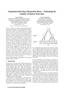
Error

Belief over states Action Measurement update Gradient Measurement model

Motion model Prediction

Observation

Fig. 1: Differentiable particle filters. Models can be learned end-to-end by backpropagation through the algorithm.

with models of the specific task. By making these algorithms differentiable and their models learnable, we can turn robotic algorithms into network architectures. This approach enables end-to-end learning while also encoding prior knowledge from algorithms, which we call algorithmic priors. Here, we apply end-to-end learning with algorithmic priors to state estimation in robotics. In this problem, a robot needs to infer the latent state from its observations and actions. Since a single observation can be insufficient to estimate the state, the robot needs to integrate uncertain information over time. Given the standard assumptions for this problem, Bayes filters provide the provably optimal algorithmic structure for solving it [21], recursively updating a probability distribution over states with prediction and measurement update using taskspecific motion and measurement models. The differentiable particle filter (DPF) is an end-to-end differentiable implementation of the particle filter—a Bayes filter that represents probability distributions with samples—with learnable motion and measurement models (see Fig. 1). Since DPFs are differentiable, we can learn their models end-to-end to optimize state estimation performance. Our experiments show that end-to-end learning improves performance compared to using models optimized for accuracy. Interestingly, end-to-end learning in DPFs re-discovers what roboticists found out via trial and error: that overestimating uncertainty is beneficial for filtering performance [21, p. 118]. Since DPFs use the Bayes filter algorithm as a prior, they have a number of advantages. First, even with end-to-

end learning, DPFs remain explainable—we can examine the learned models and their interaction. Second, the algorithmic prior regularizes learning, which greatly improves performance in state estimation. Compared to generic long short-term memory networks (LSTMs) [9], DPFs reduce the error rate by ∼80% or require 87% less training data for the same error rate. And finally, the algorithmic prior improves generalization: while LSTMs fail when tested with a different policy than used for training, DPFs are robust to changing the policy. II. R ELATED W ORK There is a surge of recent work that combines algorithmic priors and end-to-end learning for planning and state estimation with histogram-based and Gaussian belief representations. Planning with known state: Tamar et al. [20] introduced value iteration networks, a differentiable planning algorithm with models that can be optimized for value iteration. Their key insight is that value iteration in a grid based state space can be represented by convolutional neural networks. Silver et al. [18] proposed the predictron, a differentiable embedding of the TD(λ) algorithm in a learned state space. Okada and Aoshima [16] proposed path integral networks, which encode an optimal control algorithm to learn continuous tasks. State estimation (and planning) with histograms: Jonschkowski and Brock [10] introduced the end-to-end learnable histogram filter, a differentiable Bayes filter that represents the belief with a histogram. Shankar et al. [17] and Karkus et al. [11] combined histogram filters and QMDP planners in a differentiable network for planning in partially observable environments. Gupta et al. [6] combined differentiable mapping and planning in a network architecture for navigation in novel environments. All of these approaches use convolution to operate on a grid based state space. State estimation with Gaussians: Harnooja et al. [7] presented a differentiable Kalman filter with a Gaussian belief and an end-to-end learnable measurement model from visual input. Watter et al. [22] and Karl et al. [12] learn a latent state space that facilitates prediction. These approaches use (locally) linear dynamics models and Gaussian beliefs. Related work has established how to operate on histogrambased belief representations using convolution and how to work with Gaussian beliefs using linear operations. We build on this work and extend its scope to include sample-based algorithms, such as particle filters. Sample-based representations can be advantageous because they can represent multi-modal distributions (unlike Gaussians) while focusing the computational effort on states of high probability (unlike histograms). But sample-based representations introduce new challenges for differentiable implementations, e.g. generating samples from networks, performing density estimation to compute gradients, and handling non-differentiable resampling. These are the challenges that we tackle in this paper. III. BACKGROUND : BAYES F ILTERS AND T HEIR PARTICLE -BASED A PPROXIMATION We consider the problem of estimating a latent state s from a history of observations o and actions a, e.g. a robot’s pose

Fig. 2: Graphical model for state estimation

from camera images and odometry. To handle uncertainty, we estimate a probability distribution over the current state st conditioned on the history of observations o1:t and actions a1:t , which is called belief, bel(st ) = p(st |a1:t , o1:t ). A. Bayes Filters If we assume that our problem factorizes as shown in Fig. 2, the Bayes filter algorithm solves it optimally [21] by making use of the Markov property of the state and the conditional independence of observations and actions. From the Markov property follows that the last belief bel(st−1 ) summarizes all information contained in the history of observations o1:t−1 and actions a1:t−1 that is relevant for predicting the future. Accordingly, the Bayes filter computes bel(st ) recursively from bel(st−1 ) by incorporating the new information contained in at and ot . From assuming conditional independence between actions and observations given the state follows that Bayes filters update the belief in two steps: 1) prediction using action at and 2) measurement update using observation ot . 1) The prediction step is based on the motion model p(st | st−1 , at ), which defines how likely the robot enters state st if it performs action at in st−1 . Using the motion model, this step computes the predicted belief bel(st ) by summing over all st−1 from which at could have led to st . Z bel(st ) = p(st | st−1 , at ) bel(st−1 ) dst−1 . (1) 2) The measurement update uses the measurement model p(ot | st ), which defines the likelihood of an observation ot given a state st . Using this model and observation ot , this step updates the belief using Bayes’ rule (with normalization η), bel(st ) = η p(ot | st ) bel(st ).

(2)

Any implementation of the Bayes filter algorithm for a continuous state space must represent a continuous belief– and thereby approximate it. Different approximations correspond to different Bayes filter implementations, for example histogram filters, which represent the belief by a histogram, Kalman filters, which represent it by a Gaussian, or particle filters, which represent the belief by a set of particles [21]. B. Particle Filters Particle filters approximate the belief with particles (or sam[1] [2] [n] [1] [2] [n] ples) St = st , st , . . . , st with weights wt , wt , . . . , wt . The particle filter updates this distribution by moving particles, changing their weights, and resampling them, which duplicates or removes particles proportionally to their weight.

Action Belief

Resample

3

Insert particles New particles

Observ. likelihood

Particle poses

Set weights

Noisy actions

Observ. likelihood estimator

Particle proposer

Action sampler

Dynamics model

Probability density

Measurement update

2

1

0 Encoding

Particles

Observ. encoder

Particle poses

Move particles

0.0

Predicted poses

0.2

0.4 0.6 State

0.8

1.0

(b) Computing the gradient for end-to-end learning requires density estimation from the predicted particles (gray circles, Prediction darkness corresponds to particle weight). After converting the Observation particles into a mixture of Gaussians (blue), we can compute the (a) Prediction and measurement update; boxes represent models, colored boxes are learned belief at the true state (orange bar at red x) and maximize it. Predicted belief

Fig. 3: DPF overview. Models in (a) can be learned end-to-end by maximizing the belief of the true state (b).

Resampling makes this Bayes filter implementation efficient by focusing the belief approximation on probable states. The particle filter implements the prediction step (Eq. 1) by moving each particle stochastically, which is achieved by sampling from a generative motion model, [i]

[i]

∀i : st ∼ p(st | at , st−1 ).

(3)

The particle filter implements the measurement update (Eq. 2) by setting the weight of each particle to the observation likelihood—the probability of the current observation conditioned on the state represented by the particle, [i]

[i]

∀i : wt = p(ot | st ).

(4)

The particle set is then resampled by randomly drawing [i] [i] particles st proportionally to their weight wt before the filter performs the next iteration of prediction and update. IV. D IFFERENTIABLE PARTICLE F ILTERS Differentiable particle filters (DPFs) are a differentiable implementation of the particle filter algorithm with end-to-end learnable models. We can also view DPFs as a new recurrent network architecture that encodes the algorithmic prior from particle filters in the network structure (see Fig. 3a). With end-to-end learning, we do not mean that every part of a system is learned but that the objective for the learnable parts is end-to-end performance. For efficient end-to-end learning in particle filters, we need learnable models and the ability to backpropagate the gradient through the particle filter algorithm—not to change the algorithm but to compute how to change the models to improve the algorithm’s output. This section describes our DPF implementation. Our source code based on TensorFlow [1] and Sonnet [4] is available at https://github.com/tu-rbo/differentiable-particle-filters. A. Belief DPFs represent the belief at time t by a set of weighted particles, bel(st ) = (St , wt ), where S ∈ Rn×d describes n particles in d-dimensional state space with weights w ∈ Rn . At every time step, DPFs update the previous belief bel(st−1 ) with action at and observation ot to get bel(st ) (see Fig. 3a).

B. Prediction The prediction step moves each particle by sampling from a probabilistic motion model (Eq. 3). Motion models often assume deterministic environments; they account for uncertainty by generating noisy versions of the commanded or measured action such that a different version of the action is applied to each particle [21, chap. 5]. We follow the same approach by splitting the motion model into an action sampler f , which ˆ [i] per particle, and a dynamics model g, creates a noisy action a ˆ [i] . which moves each particle i according to a [i]

ˆ t = at + fθ (at , [i] ∼ N ), a

(5)

[i] st

(6)

=

[i] st−1

+

[i] [i] ˆ t ), g(st−1 , a

where fθ is a feedforward network (see Table I), θ are all parameters of the DPF, and [i] ∈ Rd is a noise vector drawn from a standard normal distribution. Using the noise vector as input for a learnable generative model is known as the reparameterization trick [14]. Here, this trick enables fθ to learn to sample from action-dependent motion noise. The resulting noisy actions are fed into g, which simulates how these actions change the state. Since we often know the underlying dynamics model, we can implement its equations in g. Alternatively, we can replace g by a feedforward network gθ and learn the dynamics from data (tested in Section V-A3). C. Measurement Update The measurement update uses the observation to compute particle weights (Eq. 4). DPFs implement this update and additionally use the observation to propose new particles (see Fig. 3a). The DPF measurement model consists of three components: a shared observation encoder h, which encodes an observation ot into a vector et , a particle proposer k, which generates new particles, and an observation likelihood estimator l, which weights each particle based on the observation. et = hθ (ot ), [i] st [i] wt

= kθ (et , δ =

(7) [i]

∼ B),

[i] lθ (et , st ),

(8) (9)

where hθ , kθ , and lθ are feedforward networks based on parameters θ; the input δ [i] is a dropout vector sampled from a Bernoulli distribution. Here, dropout is not used for regularization but as a source of randomness for sampling different particles from the same encoding et (see Table I). D. Particle Proposal and Resampling We do not initialize DPFs by uniformly sampling the state space—this would produce too few initial particles near the true state. Instead, we initialize DPFs by proposing particles from the current observation (as described above) for the first steps. During filtering, DPFs move gradually from particle proposal, which generates hypotheses, to resampling, which tracks and weeds out these hypotheses. The ratio of proposed to resampled particles follows an exponential function γ t−1 , where γ is a hyperparameter set to 0.7 in our experiments. We use 1000 particles for testing and 100 particles for training (to speed up the training process). DPFs implement resampling by stochastic universal sampling [2], which is not differentiable and leads to limitations discussed in Section IV-F. E. Supervised Learning DPF models can be learned from sequences of supervised data o1:T , a1:T , s∗1:T using maximum likelihood estimation by maximizing the belief at the true state s∗t . To estimate bel(s∗t ) from a set of particles, we treat each particle as a Gaussian in a mixture model with weights wt (see Fig. 3b). For a sensible metric across state dimensions, we scale each dimension by dividing by the average step size Et [abs(s∗t − s∗t−1 )]. This density estimation enables individual and end-to-end learning. 1) Individual learning of the motion model: We optimize the motion model individually to match the observed motion [i] noise by sampling states st from s∗t−1 and at using Eq. 56 and maximizing the data likelihood as described above, θ ∗f = argminθf − log p(s∗t | s∗t−1 , at ; θ f ). If the dynamics model g is unknown, we train gθ by minimizing mean squared error between g(s∗t−1 , at ) and s∗t − s∗t−1 . 2) Individual learning of the measurement model: The [i] particle proposer kθ is trained by sampling st from ot using Eq. 7-8 and maximizing the Gaussian mixture at s∗t . We train the observation likelihood estimator lθ (and hθ ) by maximizing the likelihood of observations in their state and minimizing their likelihood in other states, θ ∗h,l = argminθh,l − log(Et [lθ (hθ (ot ), s∗t )]) − log(1 − Et1 ,t2 [lθ (hθ (ot1 ), s∗t2 )]). 3) End-to-end learning: For end-to-end learning, we apply DPFs on overlapping subsequences and maximize the belief at all true states along the sequence as described above, θ ∗ = argminθ − log Et [bel(s∗t ; θ)]. F. Limitations and Future Work We compute the end-to-end gradient by backpropagation from the DPF output through the filtering loop. Since resampling is not differentiable, it stops the gradient computation after a single loop iteration. Therefore, the gradient neglects the effects of previous prediction and update steps on the current belief. This limits the scope of our implementation

TABLE I: Feedforward networks for learnable DPF models fθ : 2 x fc(32, relu), fc(3) + mean centering across particles gθ : 3 x fc(128, relu), fc(3) + scaled by Et [abs(st − st−1 )] hθ : conv(3x3, 16, stride 2, relu), conv(3x3, 32, stride 2, relu), conv(3x3, 64, stride 2, relu), dropout(keep 0.3), fc(128, relu) kθ : fc(128, relu), dropout*(keep 0.15), 3 x fc(128, relu), fc(4, tanh) lθ : 2 x fc(128, relu), fc(1, sigmoid scaled to range [0.004, 1.0]) fc: fully connected, conv: convolution, *: applied at training and test time

to supervised learning, where predicting the Markov state at each time step is a useful objective that facilitates future predictions. Differentiable resampling could still improve supervised learning, e.g. by encouraging beliefs to overestimate uncertainty, which reduces performance at the current step but can potentially increase robustness of future state estimates. Since it is difficult to generate training data that include the true state s∗t outside of simulation, we must work towards unsupervised learning, which will require backpropagation through multiple time steps because observations are generally non-Markov. Here are two possible implementations of differentiable resampling that could be the starting point of future work: a) Partial resampling: sample only m particles in each step; keep n−m particles from the previous time step; the gradient can flow backwards through those. b) Proxy gradients: define a proxy gradient for the weight of a resampled particle that is tied to the particle it was sampled from; the particle pose is already connected to the pose of the particle it was sampled from; the gradient can flow through these connections. V. E XPERIMENTS We evaluated DPFs in two state estimation problems in robotics: global localization and visual odometry. We tested global localization in simulated 3D mazes based on vision and odometry. We focused on this task because it requires simultaneously considering multiple hypotheses, which is the main advantage of particle filters over Kalman filters. Here, we evaluated: a) the effect of end-to-end learning compared to individual learning and b) the influence of algorithmic priors encoded in DPFs by comparing to generic LSTMs. To show the versatility of DPFs and to compare to published results with backprop Kalman filters (BKFs) [7], we also apply DPFs to the KITTI visual odometry task [5]. The goal is to track the pose of a driving car based on a first-person-view video. In both tasks, DPFs use the known dynamics model g but do not assume any knowledge about the map of the environment and learn the measurement model entirely from data. Our global localization results show that 1) algorithmic priors enable explainability, 2) end-to-end learning improves performance but sequencing individual and end-to-end learning is even more powerful, 3) algorithmic priors in DPFs improve performance compared to LSTMs reducing the error by ∼80%, and 4) algorithmic priors lead to policy invariance: While the LSTM baseline learns localization in a way that stops working when the robot behaves differently (∼84% error rate), localization with the DPF remains useful with different

Density

6 4

ind e2e ind+e2e

2 0

(d) Maze 1 observations (e) Maze 2 observations (f) Maze 3 observations

Fig. 4: Three maze environments. Red lines show example trajectories of length 100. Blue circles show the first five steps, of which the observations are depicted below.

policies (∼15% error rate). In the visual odometry task, DPFs outperform BKFs even though the task exactly fits the capabilities and limitations of Kalman filters—tracking a unimodal belief from a known initial state. This result demonstrates the applicability of DPFs to tasks with different properties: higher frequency, longer sequences, a 5D state instead of a 3D state, and latent actions. The result also shows that DPFs work on real data and are able to learn measurement models that work for visually diverse observations based on less than 40 minutes of video.

1.0 0.5 0.0 0.5 1.0 Predicted pos. relative to odom.

(a) Predictions with learned motion model (b) Comparison of learned noise

Fig. 5: Learned motion model. (a) shows predictions (cyan) of the state (red) from the previous state (black). (b) compares prediction uncertainty in x to true odometry noise (dotted line).

(a) Obs.

(b) Particle proposer

(c) Obs. likelihood estimator

0.4 0.2 (d) Obs.

(e) Particle proposer

(f) Obs. likelihood estimator

A. Global Localization Task The global localization task is about estimating the pose of a robot based on visual and odometry input. All experiments are performed in modified versions of the navigation environments from DeepMind Lab [3], where all objects and unique wall textures were removed to ensure partial observability. Data was collected by letting the simulated robot wander through the mazes (see Fig. 4). The robot followed a hand-coded policy that moves in directions with high depth values from RGBD input and performs 10% random actions. For each maze, we collected 1000 trajectories of 100 steps with one step per second for training and testing. As input for localization, we only used RGB images and odometry, both with random disturbances to make the task more realistic. For the observations, we randomly cropped the rendered 32 × 32 RGB images to 24 × 24 and added Gaussian noise (σ = 20, see Fig. 4d-f). As actions, we used odometry information that corresponds to the change in position and orientation from the previous time step in the robot’s local frame, corrupted with multiplicative Gaussian noise (σ = 0.1). All methods were optimized on short trajectories of length 20 with Adam [13] and regularized using dropout [19] and early stopping. We will now look at the results for this task. 1) Algorithmic priors enable explainability: Due to the algorithmic priors in DPFs, the models remain explainable even after end-to-end learning. We can therefore examine a) the motion model, b) the measurement model, and c) their interplay during filtering. Unless indicated otherwise, all models were first learned individually and then end-to-end.

0.8 0.6 0.4 0.2 0.0

Obs. likelihood

(c) Maze 3 (20x13)

Obs. likelihood

(b) Maze 2 (15x9)

0.0 0.8 0.6 0.4 0.2 0.0

Obs. likelihood

(a) Maze 1 (10x5)

(g) Obs.

(h) Particle proposer

(i) Obs. likelihood estimator

Fig. 6: Learned measurement model. Observations, corresponding model output, and true state (red). To remove clutter, the observation likelihood only shows above average states.

a) Motion Model: Fig. 5a shows subsequent robot poses together with predictions from the motion model. These examples show that the model has learned to spread the particles proportionally to the amount of movement, assigning higher uncertainty to larger steps. But how does this behavior depend on whether the model was learned individually or end-to-end? Fig. 5b compares the average prediction uncertainty using models from different learning schemes. The results show that individual learning produces an accurate model of the odometry noise (compare red and the dotted black lines). Endto-end learning generates models that overestimate the noise (green and orange lines), which matches insights of experts in state estimation who report that “many of the models that have proven most successful in practical applications vastly overestimate the amount of uncertainty” [21, p. 118]. b) Measurement Model: Fig. 6 shows three example observations and the corresponding outputs of the measurement model: proposed particles and weights depending on particle position. Note how the model predicts particles and estimates high weights at the true state and other states in locally symmetric parts of the maze. We can also see that the data

0.000

0.001 Particle weight

0.002

Fig. 7: Global localization with DPFs. One plot per time step of a test trajectory: true state (red), 1000 particles (proposed particles have weight 0.001). Last plot: the weighted particle mean (green) matches the true state after the first few steps.

distribution shapes the learned models, e.g. by focusing on dead ends for the second observation, which is where the robot following the hand-coded policy will look straight at a wall before turning around. Similar to motion models, end-to-end learned measurement models are not accurate but effective for end-to-end state estimation, as we will see next. c) Filtering: Figure 7 shows filtering with learned models. The DPF starts by generating many hypotheses (top row). Then, hypotheses form clusters and incorrect clusters vanish when they are inconsistent with observations (second row). Finally, the remaining cluster tracks the true state. 2) End-to-end learning improves performance: To quantify the effect of end-to-end learning on state estimation performance, we compared three different learning schemes for DPFs: individual learning of each model (ind), end-to-end learning (e2e), and both in sequence (ind+e2e). We evaluated performance in all three mazes and varied the amount of training trajectories along a logarithmic scale from 32 to 1000. We measured localization performance by error rate, where we consider a prediction erroneous if the distance to the true state, divided by Et [abs(st − st−1 )], is greater than 1. The resulting learning curves in Fig. 8a-c show that endto-end learned DPFs (orange line) consistently outperform individually trained DPFs (red line) across all mazes. Individual training is worst with few training trajectories (less than 64) but also plateaus with more data (more than 125 trajectories). In both cases, the problem is that the models are not optimized for state estimation performance. With few data, training does not take into account how unavoidable model errors affect filtering performance. With lots of data, the models might be individually accurate but suboptimal for end-

to-end filtering performance. End-to-end learning consistently leads to improved performance for the same reasons. Performance improves even more when we sequence individual and end-to-end learning (green line in Fig. 8a-c). Individual pretraining helps because it incorporates additional information about the function of each model into the learning process, while end-to-end learning incorporates information about how these models affect end-to-end performance. Naturally, it is beneficial to combine both sources of information. 3) Algorithmic priors improve performance: To measure the effect of the algorithmic priors encoded in DPFs, we compare them with a generic neural network baseline that replaces the filtering loop with a two-layer long-short-term memory network (LSTM) [9]. The baseline architecture uses the same convolutional network architecture as the DPF—it embeds images using a convolutional network hθ , concatenates the embedding with the action vector and feeds the result into 2xlstm(512), 2xfc(256, relu), and fc(3)—and is trained endto-end to minimize mean squared error. The comparison between DPF (ind+e2e) and the LSTM baseline (blue) in Fig. 8a-c shows that the error rate of DPF (ind+e2e) is lower than for LSTM for all mazes and all amounts of training data. Also in all mazes, DPF (ind+e2e) achieve the final performance of LSTM already with 125 trajectories, 18 of the full training set. We performed a small ablation study in maze 2 to quantify the effect the known dynamics model on this performance. When the dynamics model is learned, the final error rate for DPFs increases from 1.6% to 2.7% compared to 6.0% error rate for LSTMs. This shows that knowing the dynamics model is helpful but not essential for DPF’s performance.

Error rate

0.8 0.6 0.4 0.2 0.0

1.0

1.0

0.8

0.8 Error rate

LSTM DPF (ind) DPF (e2e) DPF (ind+e2e)

Error rate

1.0

0.6 0.4 0.2

16

32 64 125 250 500 Training trajectories (log. scale)

0.0

1000

16

32 64 125 250 500 Training trajectories (log. scale)

16

1.0 0.8 0.6 0.4 0.2 32 64 125 250 500 Training trajectories (log. scale)

1000

1.2 1.0 0.8 0.6 0.4 0.2 0.0

(d) Maze 1 (10x5), relative to LSTM

16

32 64 125 250 500 Training trajectories (log. scale)

(e) Maze 2 (15x9), relative to LSTM

32 64 125 250 500 Training trajectories (log. scale)

1000

(c) Maze 3 (20x13) Error rate relative to LSTM

Error rate relative to LSTM

Error rate relative to LSTM

0.0

1000

(b) Maze 2 (15x9)

1.2

16

0.4 0.2

(a) Maze 1 (10x5)

0.0

0.6

1000

1.2 1.0 0.8 0.6 0.4 0.2 0.0

16

32 64 125 250 500 Training trajectories (log. scale)

1000

(f) Maze 3 (20x13), relative to LSTM

Fig. 8: Learning curves in all mazes (a-c), also relative to LSTM baseline (d-f). ind: individual learning, e2e: end-to-end learning. Shaded areas denote standard errors.

Error rate in test with policy B A

1.0 DPF (ind) DPF (e2e) DPF (ind+e2e) LSTM

0.8

0.6

.11

.03

.01

.85

.35

.32

.26 .10

.06

.04

.03

.12

.83

0.4

0.2

.07 0.0 0.0

.13

.05 A 0.2

.08 .00 B 0.4 0.6 Trained with policy

.04

.01

.02

.01 .01 A+B 0.8

.06 1.0

Fig. 9: Generalization between policies in maze 2. A: heuristic exploration policy, B: shortest path policy. Methods were trained using 1000 trajectories from A, B, or an equal mix of A and B, and then tested with policy A or B.

To visualize the performance relative to the baseline, we divided all learning curves by LSTM’s performance (see Fig. 8df). Since DPFs encode additional prior knowledge compared to LSTMs, we might expect them to have higher bias and lower variance. Therefore, DPF’s relative error should be lowest with small amounts of data and highest with large amounts of data (the green curves in Fig. 8d-f should go up steadily from left to right until they cross the blue lines). Surprisingly, these curves show a different trend: DPFs relative performance to 1 LSTMs improves with more data and converges to about 10 1 to 3 . There could be a slight upwards trend in the end, but on a logarithmic data axis it would take a tremendous amount of data to close the gap. This result suggests that the priors

from the Bayes filter algorithm reduce variance without adding bias—that these algorithmic priors capture some true structure about the problem, which data does not help to improve upon. 4) Algorithmic priors lead to policy invariance: To be useful for different tasks, localization must be policy-invariant. At the same time, the robot must follow some policy to gather training data, which will inevitably affect the data distribution, add unwanted correlations between states and actions, etc. We investigated how much the different methods overfit to these correlations by changing the policy between training and test, using two policies A and B. Policy A refers to the heuristic exploration policy that we used for all experiments above (see Sec. V-A). Policy B uses the true pose of the robot, randomly generates a goal cell in the maze, computes the shortest path to the goal, and follows this path from cell to cell using a simple controller mixed with 10% random actions. The results in Fig. 9 show that all methods have low error rates when tested on their training policy (although DPFs improve over LSTMs even more on policy B). But when we use different policies for training and test, LSTM’s error rate jumps to over 80%, while DPF (ind+e2e) still works in most cases (5% and 26% error rate). The LSTM baseline is not able to generalize to new policies because it does not discriminate between actions and observations and fits to any information that improves state estimation. If the training data includes correlations between states and actions (e.g. because the robot moves faster in a long hallway than in a small room), then the LSTM learns this correlation. Put differently, the LSTM learns to infer the state from the action chosen by the policy. The problem is that this inference fails if the policy changes. The algorithmic priors in DPFs prevent them from overfitting to such correlations

Predicted pos. Ground truth

200

TABLE II: KITTI visual odometry results

y (m)

Test 100 0

200

400

(a) Visual input (image and difference image) at time steps 100, 200, and 300 (indicated in (b) by black circles)

0

200 x (m)

400

(b) Trajectory 9; starts at (0,0)

Fig. 10: Visual odometry with DPFs. Example test trajectory

because DPFs cannot directly infer states from actions. DPFs generalize better from A to B than from B to A. Since generalization from B to A is equally difficult for DPFs with individually learned models, the error increase cannot come from overfitting to correlations in the data through end-to-end learning but is most likely because the states visited by policy A cover those visited by policy B but not vice versa. The alternative approach to encoding policy invariance as a prior is to learn it by adding this variance to the data. Our results show that if we train on combined training data from both policies (A+B), all methods perform well in tests with either policy. This approach in the spirit of domain randomization and data augmentation helps DPFs because it covers the union of the visited states and (additionally) helps LSTM by including state-action correlations from both policies. But to make the LSTM localization truly policy invariant such that it would work with any new policy C, the training data has to cover the space of all policies in an unbiased way, which is difficult for any interesting problem. B. Visual Odometry Task To validate our simulation results on real data, we applied DPFs on the KITTI visual odometry data set, which consists of data from eleven trajectories of a real car driving in an urban area for a total of 40 minutes. The data set includes RGB stereo camera images as well as the ground truth position and orientation of the car in an interval of ∼0.1 seconds. The challenge of this task is to generalize in a way that works across highly diverse observations because the method is tested on roads that are never seen during training. Since the roads are different in each trajectory, it is not possible to extract global information about the car’s position from the images. Instead, we need to estimate the car’s translational and angular velocity from the stream of images and integrate this information over time to track the car’s position and orientation. We tackle this problem with a DPF in a five dimensional state space, which consists of the position, orientation, forward velocity and angular velocity. DPFs learn to perform visual odometry from a known initial state using a simple first-order dynamics model g and a learnable action sampler fθ . Since there is no information about the action of the driver, the action sampler produces zero mean motion noise on the velocity

Test 100/200/400/800

Translational error (m/m) BKF* DPF (ind) DPF (e2e) DPF (ind+e2e)

0.2062 0.1901 ± 0.0229 0.1467 ± 0.0149 0.1559 ± 0.0280

0.1804 0.2246 ± 0.0371 0.1748 ± 0.0468 0.1666 ± 0.0379

Rotational error (deg/m) BKF* DPF (ind) DPF (e2e) DPF (ind+e2e)

0.0801 0.1074 ± 0.0199 0.0645 ± 0.0086 0.0499 ± 0.0082

0.0556 0.0806 ± 0.0153 0.0524 ± 0.0068 0.0409 ± 0.0060

Means ± standard errors; * results from [7]

dimensions, which is then evaluated with the measurement model. For a fair comparison, we used the same network architecture for the observation encoder hθ as in the backprop Kalman filter paper [7], which takes as input the current image and the difference image to the last frame (see Fig. 10). Our observation likelihood estimator lθ weights particles based on their velocity dimensions and the encoding hθ (ot ). Since, the initial state is known, we do not use a particle proposer. We train the DPF individually and end-to-end, using only the velocity dimensions for maximum likelihood estimation. We evaluated the performance following the same procedure as in the BKF paper. We used eleven-fold cross validation where we picked one trajectory for testing and used all others for training with subsequences of length 50. We evaluated the trained model on the test trajectory by computing the average error over all subsequences of 100 time steps and all subsequences of 100, 200, 400, and 800 time steps. Table II compares our results to those published for BKFs [7]. DPFs outperform BKFs, in particular for short sequences where they reduce the error by ∼30%. Any improvement over BKFs in the this task is surprising because Gaussian beliefs seem sufficient to capture uncertainty in this task. The improvement could come from the ability of particles to represent long tailed probability distributions. These results demonstrate that DPFs generalize to different tasks and can be successfully applied to real data. VI. C ONCLUSION We introduced differentiable particle filters to demonstrate the advantages of combining end-to-end learning with algorithmic priors. End-to-end learning optimizes models for performance while algorithmic priors enable explainability and regularize learning, which improves data-efficiency and generalization. The use of algorithms as algorithmic priors will help to realize the potential of deep learning in robotics. The components of the DPF implementation, such as sample generation and density estimation, will be useful for producing differentiable versions of other sampling-based algorithms. ACKNOWLEDGMENTS We gratefully acknowledge financial support by the German Research Foundation (DFG, project number 329426068).

R EFERENCES [1] Mart´ın Abadi, Ashish Agarwal, Paul Barham, Eugene Brevdo, Zhifeng Chen, Craig Citro, Greg S. Corrado, Andy Davis, Jeffrey Dean, Matthieu Devin, Sanjay Ghemawat, Ian Goodfellow, Andrew Harp, Geoffrey Irving, Michael Isard, Yangqing Jia, Rafal Jozefowicz, Lukasz Kaiser, Manjunath Kudlur, Josh Levenberg, Dan Man´e, Rajat Monga, Sherry Moore, Derek Murray, Chris Olah, Mike Schuster, Jonathon Shlens, Benoit Steiner, Ilya Sutskever, Kunal Talwar, Paul Tucker, Vincent Vanhoucke, Vijay Vasudevan, Fernanda Vi´egas, Oriol Vinyals, Pete Warden, Martin Wattenberg, Martin Wicke, Yuan Yu, and Xiaoqiang Zheng. TensorFlow: Largescale machine learning on heterogeneous systems. http: //tensorflow.org/, 2015. [2] James E. Baker. Reducing Bias and Inefficiency in the Selection Algorithm. In Proceedings of the International Conference on Genetic Algorithms (ICGA), pages 14–21, 1987. [3] Charles Beattie, Joel Z. Leibo, Denis Teplyashin, Tom Ward, Marcus Wainwright, Heinrich K¨uttler, Andrew Lefrancq, Simon Green, V´ıctor Vald´es, Amir Sadik, and others. Deepmind Lab. arXiv:1612.03801, 2016. [4] DeepMind. Sonnet: TensorFlow-Based Neural Network Library. https://github.com/deepmind/sonnet, 2017. [5] Andreas Geiger, Philip Lenz, Christoph Stiller, and Raquel Urtasun. Vision Meets Robotics: The KITTI Dataset. The International Journal of Robotics Research, 32(11):1231–1237, 2013. [6] Saurabh Gupta, James Davidson, Sergey Levine, Rahul Sukthankar, and Jitendra Malik. Cognitive Mapping and Planning for Visual Navigation. arXiv:1702.03920, 2017. [7] Tuomas Haarnoja, Anurag Ajay, Sergey Levine, and Pieter Abbeel. Backprop KF: Learning Discriminative Deterministic State Estimators. In Advances in Neural Information Processing Systems (NIPS), pages 4376– 4384, 2016. [8] Kaiming He, Xiangyu Zhang, Shaoqing Ren, and Jian Sun. Deep Residual Learning for Image Recognition. arXiv:1512.03385, 2015. [9] Sepp Hochreiter and J¨urgen Schmidhuber. Long ShortTerm Memory. Neural Computation, 9(8):1735–1780, 1997. [10] Rico Jonschkowski and Oliver Brock. End-To-End Learnable Histogram Filters. In Workshop on Deep Learning for Action and Interaction at the Conference on Neural Information Processing Systems (NIPS), 2016.

[11] Peter Karkus, David Hsu, and Wee Sun Lee. QMDP-Net: Deep Learning for Planning under Partial Observability. In Advances in Neural Information Processing Systems (NIPS), pages 4697–4707, 2017. [12] Maximilian Karl, Maximilian Soelch, Justin Bayer, and Patrick van der Smagt. Deep Wariational Bayes Filters: Unsupervised Learning of State Space Models from Raw Data. arXiv:1605.06432, 2017. [13] Diederik P. Kingma and Jimmy Ba. Adam: A Method for Stochastic Optimization. In Proceedings of the International Conference on Learning Representations (ICLR), 2014. [14] Diederik P. Kingma and Max Welling. Auto-Encoding Variational Bayes. arXiv:1312.6114, 2013. [15] Yann A. LeCun, Bernhard E. Boser, John S. Denker, Donnie Henderson, Richard E. Howard, Wayne E. Hubbard, and Lawrence D. Jackel. Backpropagation Applied to Handwritten Zip Code Recognition. Neural Computation, 1(4):541–551, 1989. [16] Masashi Okada, Luca Rigazio, and Takenobu Aoshima. Path Integral Networks: End-to-End Differentiable Optimal Control. arXiv:1706.09597, 2017. [17] Tanmay Shankar, Santosha K. Dwivedy, and Prithwijit Guha. Reinforcement Learning via Recurrent Convolutional Neural Networks. In Proceedings of the International Conference on Pattern Recognition (ICPR), pages 2592–2597, 2016. [18] David Silver, Hado van Hasselt, Matteo Hessel, Tom Schaul, Arthur Guez, Tim Harley, Gabriel Dulac-Arnold, David Reichert, Neil Rabinowitz, and Andre Barreto. The Predictron: End-to-End Learning and Planning. In Proceedings of the International Conference on Machine Learning (ICML), pages 3191–3199, 2017. [19] Nitish Srivastava, Geoffrey Hinton, Alex Krizhevsky, Ilya Sutskever, and Ruslan Salakhutdinov. Dropout: A Simple Way to Prevent Neural Networks from Overfitting. Journal of Machine Learning Research, 15(1):1929–1958, 2014. [20] Aviv Tamar, Yi Wu, Garrett Thomas, Sergey Levine, and Pieter Abbeel. Value Iteration Networks. In Advances in Neural Information Processing Systems (NIPS), pages 2154–2162, 2016. [21] Sebastian Thrun, Wolfram Burgard, and Dieter Fox. Probabilistic Robotics. MIT Press, 2005. [22] Manuel Watter, Jost Tobias Springberg, Joschka Boedecker, and Martin Riedmiller. Embed to Control: A Locally Linear Latent Dynamics Model for Control from Raw Images. In Advances in Neural Information Processing Systems (NIPS), pages 2746–2754, 2015.