Local Ensemble Kalman Particle Filters for efficient data ... - arXiv

Localization in High-Dimensional Monte Carlo Filtering

arXiv:1610.03701v2 [stat.CO] 22 Dec 2016

Sylvain Robert and Hans R. Künsch

Abstract The high dimensionality and computational constraints associated with filtering problems in large-scale geophysical applications are particularly challenging for the Particle Filter (PF). Approximate but efficient methods such as the Ensemble Kalman Filter (EnKF) are therefore usually preferred. A key element of these approximate methods is localization, which is a general technique to avoid the curse of dimensionality and consists in limiting the influence of observations to neighboring sites. However, while it works effectively with the EnKF, localization introduces harmful discontinuities in the estimated physical fields when applied blindly to the PF . In the present paper, we explore two possible local algorithms based on the Ensemble Kalman Particle Filter (EnKPF), a hybrid method combining the EnKF and the PF. A simulation study in a conjugate normal setup allows to highlight the tradeoffs involved when applying localization to PF algorithms in the high-dimensional setting. Experiments with the Lorenz96 model demonstrate the ability of the local E n KPF algorithms to perform well even with a small number of particles compared to the problem size.

1 Introduction Monte Carlo methods are becoming increasingly popular for filtering in large-scale geophysical applications, such as reservoir modeling and numerical weather prediction, where they are often called ensemble methods for data assimilation. The challenging (and interesting) peculiarity of this type of applications is that the state space is extremely high dimensional (the number of dimensions of the state x is typically of the order of 108 and the dimension of the observation y of the order of 106 ), while the computational cost of the time integration step limits the sample size to less than a hundred. Because of those particularly severe constraints, the emphasis is on developing approximate but highly efficient methods, typically relying on strong assumptions and exploiting parallel architectures.

1

2


The Particle Filter (PF) provides a fully general Bayesian solution to filtering [6, 14, 1], but it is well-known that it suffers from sample degeneracy and cannot be applied to high-dimensional settings [17]. The most popular alternative to the PF in large-scale applications is the Ensemble Kalman Filter (EnKF) [2, 3], a successful but heuristic method, which implicitly assumes that the predictive distribution is Gaussian. Three main routes for adapting the PF to high-dimensional settings can be identified. The first one is to use an adaptive PF with a carefully chosen proposal distribution [14, 10]. A second approach is to build hybrid methods between the EnKF and the PF, as for example the Ensemble Kalman Particle Filter (EnKPF) [4]. A third route is localization, as it is a key element of the success of the EnKF in practice and could avoid the curse of dimensionality [17, 15]. The first approach requires an explicit model for the transition probabilities, which is typically not available in practical applications. Furthermore [18] showed that even with the optimal proposal distribution the PF suffers from the curse of dimensionality. Therefore in the present paper we focus on the second and third approaches and explore some possible localized algorithms based on the PF and the E n KPF . In a simulation study, we extend an example of [17] to illustrate how localization seemingly overcomes the curse of dimensionality, but at the same time introduces some harmful discontinuities in the estimated state. In a second experiment we show how local algorithms can be applied effectively to a filtering problem with the Lorenz96 model [11]. The results from these numerical experiments highlight key differences between the algorithms and demonstrate that local EnKPFs are promising candidates for large-scale filtering applications.

2 Ensemble filtering algorithms Consider a state space model with state process (xt ) and observations (yt ), where the state process evolves according to some deterministic or stochastic dynamics and the observations are assumed to be independent given the state process, with likelihood p(xt |yt ). The goal is to estimate the conditional distribution of xt given y1:t = (y1 , . . . , yt ), called the filtering distribution and which we denote by πtf . In general it is possible to solve this problem recursively by alternating between a prediction step where the filtering distribution at time (t − 1) is propagated into the predictive distribution πtp at time t, and an update step, also called assimilation, where the predictive distribution is updated with the current observation to compute πtf . The update step is done by applying Bayes’ rule as πtf (x) ∝ πtp (x) · p(x|yt ), where the predictive distribution is the prior and the filtering distribution the posterior to be estimated. Sequential Monte Carlo methods [1] approximate the predictive and filtering distributions by finite samples, or ensembles of particles, denoted by (xtp,i ) and (xtf ,i ) respectively, for i = 1, . . . , k. The update step consists in transforming the predictive ensemble (xtp,i ) into an approximate sample from the filtering distribution πtf . We


3

briefly present the PF and EnKF in this context and give an overview of the EnKPF. Henceforth we consider the update step only and drop the time index t. Additionally for the EnKF and EnKPF we assume that the observations are linear and Gaussian, i.e. p(x|y) = φ (y; Hx, R), the Gaussian density with mean Hx and covariance R evaluated at y. The Particle Filter approximates the filtering distribution as a mixture of point masses at the predictive particles, reweighed by their likelihood. More precisely: k

f πˆPF (x) = ∑ wi δx p,i (x),

wi ∝ φ (y; Hx p,i , R).

(1)

i=1

A non-weighted sample from this distribution can be obtained by resampling, for example with a balanced sampling scheme [9]. The PF is asymptotically correct (also for non-Gaussian likelihoods), but to avoid sample degeneracy it needs a sample size which increases exponentially with the size of the problem (for more detail see [17]). The Ensemble Kalman Filter is a heuristic method which applies a Kalman Filter (KF) update to each particle with stochastically perturbed observations. More precisely it constructs (x f ,i ) as a balanced sample from the following Gaussian mixture: k

1 ˆ − Hx p,i ), KR ˆ Kˆ 0 ), φ (x; x p,i + K(y k i=1

f (x) = ∑ πÊnKF

(2)

where Kˆ is the Kalman gain estimated with Σˆ p , the sample covariance of (x p,i ): The stochastic perturbations of the observations are added to ensure that the filter ensemble has the correct posterior covariance on expectation. The Ensemble Kalman Particle Filter combines the EnKF and the PF by decomposing the update step into two stages as π f (x) ∝ π p (x) · p(x|y)γ · p(x|y)1−γ , following the progressive correction idea of [12]. The first stage, going from π p (x) to π γ (x) ∝ π p (x) · p(x|y)γ is done with an EnKF. The second stage is done with a PF and goes from π γ (x) to π f (x) ∝ π γ (x) · p(x|y)1−γ . The resulting posterior distribution can be derived analytically as the following weighted Gaussian mixture: k

f (x) = ∑ α γ,i φ (x; µ γ,i , Σ γ ), πÊnKPF

(3)

i=1

where the expressions for the parameters of this distribution and more details on the algorithm can be found in [4]. To produce the filtering ensemble (x f ,i ), one first samples the mixture components with probability proportional to the weights α γ,i , using for example a balanced sampling scheme, and then adds an individual noise term with covariance Σ γ to each particle. The parameter γ defines a continuous interpolation between the PF (γ = 0) and the EnKF (γ = 1). In the present study the value of γ is either fixed, for the sake of comparison, or chosen adaptively. In the later case γ is chosen such that the equivalent sample size of the filtering

4


ensemble is within some acceptable range. Alternative schemes for choosing γ such as minimizing an objective cost function are currently being investigated but are beyond the scope of this work.

3 Local algorithms Localization consists essentially in updating the state vector by ignoring long range dependencies. This is a sensible thing to do in geophysical applications where the state represents discretized spatially correlated fields of physical quantities. By localizing the update step and using local observations only, one introduces a bias, but achieves a considerable gain in terms of variance reduction for finite sample sizes. For local algorithms the error is asymptotically bigger than for a global algorithm, but it is not dependent on the system dimension anymore and therefore avoids the curse of dimensionality. Furthermore, local algorithms can be efficiently implemented in parallel and thus take advantage of modern computing architectures. The Local E N KF (LEnKF) consists in applying a separate EnKF at each site, but limiting the influence of the observations to sites that are spatially close (there are different ways to accomplish this in practice, see for example [7, 13, 8]). Analogously, we define the local PF (LPF) as a localized version of the PF, where the update is done at each location independently, considering only observations in a ball of radius `. In order to avoid arbitrary “scrambling” of the particles indices, we use a balanced sampling scheme [9], and some basic ad-hoc methods to reduce the number of discontinuities, but we do not solve this problem optimally as it would greatly hinder the efficiency of the algorithm. For the EnKPF we define two different local algorithms: the naive-local EnKPF (NAIVE - LEnKPF), in which localization is done exactly as for the LEnKF, and the block-local EnKPF (BLOCK - LEnKPF), in which the observations are assimilated sequentially but their influence is restricted to a local area. The NAIVE - LEnKPF does not take particular care of the introduced discontinuities beyond what is done for the PF , but it is straightforward to implement. The BLOCK - LE n KPF , on the other hand, uses conditional resampling in a transition area surrounding the local assimilation window, which ensures that there are no sharp discontinuities, but it involves more overhead computation. For more detail about the local EnKPF algorithms see [16].

4 Simulation studies We conducted two simulation studies: first a one-step conjugate normal setup where the effect of localization can be closely studied, and second a cycled experiment with the Lorenz96 model, a non-linear dynamical system displaying interesting nonGaussian features.


5

4.1 Conjugate normal setup We consider a simple setup similar to the one in [17], with a predictive distribution π p assumed to be a N-dimensional normal with mean zero and covariance Σ p . To imitate the kind of smooth fields that we encounter in geophysical applications, we construct the covariance matrix as Σiip = 1 and Σipj = KGC (d(i, j)/r), where KGC is the Gaspari-Cohn kernel [5], d(i, j) the distance between sites i and j on a onedimensional domain with periodic boundary conditions, and the radius r in the denominator is chosen such that the covariance has a finite support of 20 grid points. From this process we generate observations of every component of x and standard Gaussian noise: x ∼ N (0, Σ p ),

y|x ∼ N (x, I).

(4)

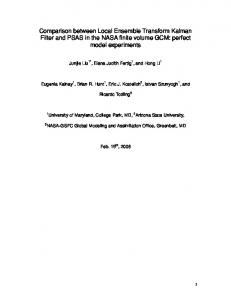
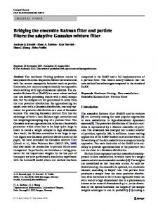
In order to study the finite sample properties of the different algorithms, we compute the Mean Squared Error (MSE) of the ensemble mean in estimating the value x at each location, which we denote by MSE(x). Because the prior is conjugate to the likelihood, we can compute the MSE(x) of the posterior mean analytically for known Σ p as the trace of the posterior covariance matrix and use this as a reference. For the simulation we use a sample size of k = 100 and average the results over 1000 runs. It should be noted that because the predictive distribution is normal, this setup is favorable to the EnKF and LEnKF, but the EnKPFs should still perform adequately. For the local algorithms the localization radius ` was set to 5, resulting in a local window of 11 grid points, which is smaller than the correlation length used to generate the data. Later on we study the effect of ` on the performance of the algorithms. For the EnKPF algorithms the parameter γ was fixed to 0.25, which means a quarter of EnKF and three-quarter of PF. In practice one would rather choose the value of γ adaptively, but the exact value does not influence the qualitative conclusions drawn from the experiments and fixing it in this way makes the comparison easier. An example of a sample from the filtering distribution produced by different local algorithms is shown in fig. 1, with each particle represented as a light blue line, the true state in dark and the observations in red. For more clarity the ensemble size is set to 10 and the system dimension to 40. While all algorithms manage to recover more or less the underlying state, it is clear that they vary in terms of quality. The LPF in particular suffers from sample depletion, even when applied locally, and displays strong discontinuities. If one looks closely at the NAIVE - LEnKPF ensemble, discontinuities can also be identified. The BLOCK - LEnKPF and the LEnKF, on the other hand, produce smoother posterior particles. This example is useful to highlight the behavior of the different local algorithms qualitatively, but we now proceed to a more quantitative assessment with a repeated simulations experiment. Beating the curse of dimensionality: In the first row of fig. 2, the MSE(x) is plotted as a function of the system dimension N, for the global algorithms on the left and the local algorithms on the right. The values are normalized by the optimal MSE(x) to make them more interpretable. The PF degenerates rapidly, with an MSE(x) worse than using the prior mean (upper dashed line). The EnKF and the EnKPF suffer as

6

Sylvain Robert and Hans R. Künsch LEnKF

LPF

block-LEnKPF

naive-LEnKPF

2.5

value

0.0

-2.5

2.5

0.0

-2.5 0

10

20

30

40

0

10

20

30

40

Location

Fig. 1 Example of analysis ensemble with different local algorithms. Each particle is a light blue line, the true state in dark and the observations in red. The ensemble size is restricted to 10 and the domain size to 40 for better legibility.

well from the curse of dimensionality, although to a lesser extent. The local algorithms, on the other hand, are immune to the increase of dimensions N and their MSE(x) is constant and very close the optimum, which confirms that localization is working as expected. The LEnKF, NAIVE - LEnKPF and BLOCK - LEnKPF make an error of less than 5% while the LPF is 20% worse than the optimum. Global

Local

8 EnKF

relative MSE(x)

6

8

LEnKF

6

LPF

PF 4

block-LEnKPF

4

EnKPF

2

naive-LEnKPF

2

0

500

1000

1500

0

500

N

1000

Local

3.0

3.0 EnKF

relative MSE(Δx)

1500

N

Global

2.5

LEnKF 2.5

PF EnKPF

2.0

LPF block-LEnKPF

2.0

naive-LEnKPF 1.5

1.5

1.0

1.0 0

500

1000

N

1500

0

500

1000

1500

N

Fig. 2 Illustration of the relationship between the system dimension N and different quantities. In the first row is the MSE(x) for the global algorithms on the left and the local algorithms on the right. In the second row the same but for the MSE(∆ x). All the values are given relative to the optimal one obtained with the true posterior distribution (dashed line at 1). The relative MSE of using the prior without using any observation is given by the second dashed line. Notice the log-scale on the y-axis.

The cost of localization: As the old statistical adage goes, there is no free lunch: localization comes at a cost, particularly for PF algorithms. When doing the update locally with the EnKF, the filtering samples are relatively smooth fields, because the


7

update applies spatially smoothly varying corrections to the predictive ensemble. However, for the LPF, when different particles are resampled at neighboring sites, arbitrarily large discontinuities can be created. While this might be discarded as harmless, it is not the case when the fields of interest are spatial fields of physical quantities used in numerical solvers of partial differential equations. One way to measure the impact of discontinuities is to look at the MSE in estimating the lag one increments ∆ x, which we denote as MSE(∆ x). While the MSE(x) is computed for the posterior mean, the MSE(∆ x) is computed for each particle separately and then averaged. We again compute the expected MSE(∆ x) under the conjugate posterior distribution and use it as reference. The plots in the second row of fig. 2 show this quantity for the different algorithms averaged over 1000 simulation runs. The MSE(∆ x) of the local algorithms is still constant as a function of N, as expected, but in the cases of the NAIVE - LEnKPF and the LPF its value is worse than for the respective global algorithms. On the other hand, the LEnKF and the BLOCK - LEnKPF improve on their global counterparts and have an error relatively close to the optimum. Localization trade-off: In the previous experiment we fixed `, the localization radius, to 5, and looked at what happens in terms of prediction accuracy with the MSE (x), and in terms of discontinuities with the MSE (∆ x). In fig. 3 we now look at MSE as a function of `, fixing N to 200 and k to 100. For large values of ` the MSE (∆ x) is smallest as discontinuities are avoided, but the MSE(x) is not optimal, particularly for the LPF. As ` is reduced the MSE(x) decreases for all methods, while MSE (∆ x) is kept constant for a wide range of ` values. At some point, different for each algorithm, the localization is too strong and becomes detrimental, with both MSE (x) and MSE (∆ x) sharply increasing. This behavior illustrates the trade-off at hand when choosing the localization radius: picking a too small value introduces a bias by neglecting useful information and creates too much discontinuities, while choosing a too large value does not improve MSE(∆ x) but leads to poorer performance in terms of MSE(x). MSE(x)

MSE(Δx)

8

3.0

LEnKF 6

LPF

2.5

Relative MSE

Relative MSE

block-LEnKPF 4

naive-LEnKPF

2

2.0

1.5

1.0 0

10

20

30

Localization radius

40

50

0

10

20

30

40

50

Localization radius

Fig. 3 Trade-off of localization: influence of ` on MSE(x) and MSE(∆ x) for the local algorithms. The ensemble size k was fixed to 100 and the system dimension N to 200. Notice the log-scale on the y-axis.

8


4.2 Filtering with the Lorenz96 model The Lorenz96 model [11] is a 40-dimensional non-linear dynamical system which displays a rich behavior and is often used as a benchmark for filtering algorithms. In [4] it was shown that the EnKPF outperforms the LEnKF in some setups of the Lorenz96 model, but the sample size required was of 400. In the present experiment we use the same setup as in [4] but with much smaller and realistic ensemble sizes. The data are assimilated at time intervals of 0.4, which leads to strong non-linearities and thus highlights better the relative advantages of the EnKPF. Each experiment is run for 1000 cycles and repeated 20 times, which provides us with stable estimates of the average performance of each algorithm. As in [4], the parameter γ of the E n KPF s is chosen adaptively such that the equivalent sample size is between 25 and 50% of the ensemble size. It should be noted that for local algorithms, a different γ is chosen at each location, which provides added flexibility and allows to adapt to locally non-Gaussian features of the distribution. We consider MSE(x) only and denote it simply by MSE. It also takes errors in the estimation of increments into account through integration in time during the propagation steps. In the left panel of fig. 4 the MSE of the global algorithms is plotted against ensemble size. The PF is not represented as it diverges for such small values. The MSE is computed relative to the performance of the prior, which is simply taken as the MSE of an ensemble of the same size evolving according to the dynamical system equations but not assimilating any observations. With ensemble sizes smaller than 50, the filtering algorithms are not able to do better than the prior, which means that trying to use the observations actually makes them worse than not using them at all. Only for ensemble sizes of 100 and more do the global algorithms start to become effective. In practice we are interested in situations where the ensemble size is smaller than the system dimension (here 40), and thus the global methods are clearly not applicable. On the right panel of fig. 4 we show the same plot but for the local algorithms. For sample sizes as small as 20 or 30 the performances are already quite good. The LPF , however, does not work at all, probably because it still suffers from sample depletion and because the discontinuities it introduces have a detrimental impact during the prediction step of the algorithm. The BLOCK - LEnKPF clearly outperforms the other algorithms, particularly for smaller sample sizes. This indicates that it can localize efficiently the update without harming the prediction step by introducing discontinuities in the fields. In order to better highlight the trade-off of localization, we plot similar curves but as a function of the localization radius ` in fig. 5. One can see that for small k (left panel), the error is increasing with `, which shows that localization is absolutely necessary for the algorithm to work. For k = 40 (right panel), the MSE first decreases and then increases, with an optimal `. Experiments with larger values display curves that get flatter and flatter as k increases, showing that as the ensemble size is larger, the localization strength needed is smaller, as expected.


9

Global

Local

2.0

2.0

1.5

1.5

1.0

1.0

Relative MSE

Relative MSE

LEnKF EnKF

0.5

EnKPF

25

50

75

LPF

0.5

block-LEnKPF naive-LEnKPF

100

25

50

k

75

100

k

Fig. 4 Global and local algorithms results with the Lorenz96 model. On the y-axis the MSE and on the x-axis increasing ensemble sizes k. There is no global PF as the algorithm does not work for such small ensemble sizes. The MSE is computed relative to the MSE of an ensemble of the same size but which does not assimilate any observation. Notice the log-scale on the y-axis. k=10

k=40

2.0 1.5

Relative MSE

1.0 LEnKF 0.5

LPF block-LEnKPF naive-LEnKPF

2.5

5.0

7.5

10.0

2.5

5.0

7.5

10.0

Localization radius

Fig. 5 Interplay of ensemble size k and localization radius ` for the the Lorenz96 model. The relative MSE is plotted as a function of ` for different value of k in the different panels. Notice the log-scale on the y-axis.

5 Conclusion Localization is an effective tool to address some of the difficulties associated with high-dimensional filtering in large-scale geophysical applications. Methods such as the EnKF can be localized easily and successfully as they vary smoothly in space. At first sight, the LPF does seem to overcome the curse of dimensionality; however, looking more carefully, one notices that it introduces harmful discontinuities in the updated fields. The two localized EnKPFs both overcome the curse of dimensionality and handle better the problem of discontinuities. The simple conjugate example studied in this paper highlighted the potential improvements coming from localization, as well as the pitfalls when applied blindly to the PF. The trade-off between the bias coming from localization and the gain coming from the reduced variance was illustrated by exploring the behavior of the algorithms as a function of the localization radius `. Experiments with the Lorenz96 model showed that local algorithms can be successfully applied with ensemble sizes as small as 20 or 30, and highlighted the localization trade-off. In particular, the BLOCK - LEn KPF fared remarkably well, outperforming both the NAIVE - LEn KPF and the LEnKF in this challenging setup. This confirms other results that we obtained with more complex dynamical models mimicking cumulus convection [16] and en-

10


courages us to pursue further research with localized EnKPFs in a large-scale application in collaboration with Meteoswiss.

References 1. Doucet, A., De Freitas, N., Gordon, N.: Sequential Monte Carlo Methods in Practice. Springer New-York (2001) 2. Evensen, G.: Sequential data assimilation with a nonlinear quasi-geostrophic model using Monte Carlo methods to forecast error statistics. Journal of Geophysical Research: Oceans 99(C5), 10,143–10,162 (1994) 3. Evensen, G.: The ensemble Kalman filter: theoretical formulation and practical implementation. Ocean Dynamics 53(4), 343–367 (2003) 4. Frei, M., Künsch, H.R.: Bridging the ensemble Kalman and particle filters. Biometrika 100(4), 781–800 (2013) 5. Gaspari, G., Cohn, S.E.: Construction of correlation functions in two and three dimensions. Quarterly Journal of the Royal Meteorological Society 125(554), 723–757 (1999) 6. Gordon, N., Salmond, D., Smith, A.: Novel approach to nonlinear non-Gaussian Bayesian state estimation. Radar and Signal Processing, IEE Proceedings F 140(2), 107–113 (1993) 7. Houtekamer, P.L., Mitchell, H.L.: A sequential ensemble Kalman filter for atmospheric data assimilation. Monthly Weather Review 129(1), 123–137 (2001) 8. Hunt, B.R., Kostelich, E.J., Szunyogh, I.: Efficient data assimilation for spatiotemporal chaos: A local ensemble transform Kalman filter. Physica D: Nonlinear Phenomena 230(1-2), 112– 126 (2007) 9. Künsch, H.R.: Recursive Monte Carlo filters: Algorithms and theoretical analysis. The Annals of Statistics 33(5), 1983–2021 (2005) 10. van Leeuwen, P.J.: Nonlinear data assimilation in geosciences: an extremely efficient particle filter. Quarterly Journal of the Royal Meteorological Society 136(653), 1991–1999 (2010) 11. Lorenz, E.N., Emanuel, K.A.: Optimal sites for supplementary weather observations: Simulation with a small model. Journal of the Atmospheric Sciences 55(3), 399–414 (1998) 12. Musso, C., Oudjane, N., Le Gland, F.: Improving regularised particle filters. In: A. Doucet, N. De Freitas, N. Gordon (eds.) Sequential Monte Carlo Methods in Practice, pp. 247–271. Springer New-York (2001) 13. Ott, E., Hunt, B.R., Szunyogh, I., Zimin, A.V., Kostelich, E.J., Corazza, M., Kalnay, E., Patil, D.J., Yorke, J.A.: A local ensemble Kalman filter for atmospheric data assimilation. Tellus A 56(5), 415–428 (2004) 14. Pitt, M.K., Shephard, N.: Filtering via simulation: Auxiliary particle filters. Journal of the American Statistical Association 94(446), 590–599 (1999) 15. Rebeschini, P., Handel, R.v.: Can local particle filters beat the curse of dimensionality? The Annals of Applied Probability 25(5), 2809–2866 (2015) 16. Robert, S., Künsch, H.R.: Local ensemble Kalman particle filters for efficient data assimilation. ArXiv:1605.05476 (2016) 17. Snyder, C., Bengtsson, T., Bickel, P., Anderson, J.: Obstacles to high-dimensional particle filtering. Monthly Weather Review 136(12), 4629–4640 (2008) 18. Snyder, C., Bengtsson, T., Morzfeld, M.: Performance bounds for particle filters using the optimal proposal. Monthly Weather Review 143(11), 4750–4761 (2015)