Diffusion Maps and Coarse-Graining: A Unified ... - CiteSeerX

1

Diffusion Maps and Coarse-Graining: A Unified Framework for Dimensionality Reduction, Graph Partitioning and Data Set Parameterization Stéphane Lafon1 and Ann B. Lee2 1 Google Inc., [email protected]. 2 Department of Statistics, Carnegie Mellon University, [email protected]. Abstract We provide evidence that non-linear dimensionality reduction, clustering and data set parameterization can be solved within one and the same framework. The main idea is to define a system of coordinates with an explicit metric that reflects the connectivity of a given data set and that is robust to noise. Our construction, which is based on a Markov random walk on the data, offers a general scheme of simultaneously reorganizing and subsampling graphs and arbitrarily shaped data sets in high dimensions using intrinsic geometry. We show that clustering in embedding spaces is equivalent to compressing operators. The objective of data partitioning and clustering is to coarse-grain the random walk on the data while at the same time preserving a diffusion operator for the intrinsic geometry or connectivity of the data set up to some accuracy. We show that the quantization distortion in diffusion space bounds the error of compression of the operator, thus giving a rigorous justification for k-means clustering in diffusion space and a precise measure of the performance of general clustering algorithms. Index Terms Machine learning, Text analysis, Knowledge retrieval, Quantization, Graph-theoretic methods, Compression (coding), Clustering, Clustering similarity measures, Information visualization, Markov processes, Graph algorithms

I. I NTRODUCTION When dealing with data in high dimensions, one is often faced with the problem of how to reduce the complexity of a data set while preserving information that is important for, for example, understanding the data structure itself or for performing later tasks such as clustering, classification and regression. Dimensionality or complexity reduction is an ill-posed problem until one clearly defines what one is ready to lose. In this work, we attempt to find both a parameterization and an explicit metric that reflects the intrinsic geometry of a given data set. With intrinsic geometry, we here mean a set of rules that describe the relationship between the objects in the data set without reference to structures outside of it; in our case, we define intrinsic geometry by the connectivity of the data points in a diffusion process. One application of this work, is manifold learning where we have a manifold, say a 2D “Swiss roll”, embedded in a higher-dimensional space — but more generally, the problems of data parameterization, dimensionality reduction and clustering extend beyond manifold learning to general graphs of objects that are linked by edges with weights. There is a large body of literature regarding the use of the spectral properties (eigenvectors and eigenvalues) of a pairwise similarity matrix for geometric data analysis. These methods can roughly be divided into two main categories: spectral graph cuts [1], [2], [3] and eigenmaps [4], [5], [6], [7]. The two methodologies were originally developed for different types of applications: segmentation and partitioning of graphs versus locality-preserving embeddings of data sets, respectively. Below we briefly review previous work and how it relates to the diffusion framework. Suppose that Ω = {x1 , ..., xn } is a data set of points, and assume that these points form the nodes of a weighted graph with weight function w(x, y). In the graph-theoretic approach [8] to data partitioning,

2

one seeks to divide the set of vertices into disjoint sets, where by some measure, the similarity among the vertices in a set is high, and the similarity across different sets is low. Different algorithm use different matrices but, in general, these spectral grouping methods are based on an analysis of the dominant eigenvectors of a suitably normalized weight matrix (see e.g. [1] for a review). If the weight function w(x, y) satisfies certain conditions (symmetry and pointwise positivity), then one can interpret the pairwise similarities as edge flows in a Markov random walk on the graph. In this probabilistic formulation, the transition probability of going from point x to y in one step is w(x, y) . z∈Ω w(x, z)

p(x, y) = P

The Normalized Cut problem provides a justification and some intuition for the use of the first nontrivial eigenfunction of the random walk’s transition matrix [2]; the authors Shi and Malik also mention using higher-order eigenfunctions but do not provide a theoretical justification for such an analysis. More recently, Meila and Shi [3] have shown that the transition matrix P has piecewise constant eigenvectors relative to a partition S = (S1 , S2 , . . . , Sk ) when the underlying Markov chain is lumpable with respect to S, i.e. when one is able to group vertices together due to similarities of their transition probabilities to the subsets Sj . The authors also define a “Modified Ncut” algorithm which, for the special case of lumpable Markov chains, finds all k segments by k-means of the eigenvectors of P . Despite recent progress in the field of spectral graph theory, there are still many open questions. In particular: What is the intuition behind spectral clustering when eigenvectors are not piece-wise constant (and Markov chains are not lumpable)? Naturally occuring data sets only display, at best, approximate lumpability; the issue then is whether we can say something more precise about the performance of various clustering algorithms. Furthermore, for general data sets, which eigenvectors of the Markov matrix should be considered and what is the relative importance of these? Below, we answer these questions by unifying ideas in spectral clustering, operator compression and data set parameterization. The problem of spectral clustering is very closely related to the problem of finding low-dimensional locality-preserving embeddings of data sets. For example, suppose that we wish to find an embedding of Ω in Rp according to x 7→ f (x) = (f1 (x), . . . , fp (x)) that preserves the local neighborhood information. Several algorithms, such as LLE [4], Laplacian eigenmaps [6], Hessian eigenmaps [7], LTSA [5] and diffusion maps [9], [10], all aim at minimizing distortions P of the form Q(f ) = i Qi (f ) where Qi (f ) is a symmetric, positive semi-definite quadratic form that measures local variations of f around xi . The p-dimensional embedding problem can, in these cases, be rewritten as an eigenvalue problem where the first p eigenvectors (f1 , ..., fp ) provide the optimal embedding coordinates. The close relationship between spectral clustering and locality-preserving dimension reduction has, in particular, been pointed out by Belkin and Niyogi. In [6], the authors show that the Laplacian of a graph (whose eigenvectors are used in spectral cuts) is the discrete analogue of the Laplace-Beltrami operator on manifolds, and the eigenfunctions of the latter operator have properties desired for embeddings. However, as in the case of spectral clustering, the question of the number of eigenvectors in existing eigenmap methods is still open. Furthermore, as the distance metric in the embedding spaces is not explicitly defined, it is not clear how one should cluster and partition data. The usual approach is: First pick a dimension k, then calculate the first k non-trivial eigenvectors and weight these equally in clustering and other subsequent data analysis. The contribution of this paper is two-fold: First, we provide a unified framework for spectral data analysis based on the idea of diffusion and put previous work in a new perspective. Our starting point is an explicit metric that reflects the connectivity of the data set. This so called “diffusion metric” can be explained in terms of transition probabilities of a Markov chain that evolves forward in time and is, unlike the geodesic distance, or the shortest path of a graph, very robust to noise. Similar distance measures have previously been suggested in clustering and data classification, see for example [11]. However, the

3

Methods for clustering and non-linear dim. reduction Spectral graphs [1], [2], [3] Eigenmaps [4], [5], [6], [7] Isomap [13] Markov random walk learning [11] Diffusion maps

data set parameterization? not directly addressed yes yes no yes

explicit metric in embedding space? no no yes yes yes

TABLE I A SIMPLIFIED TABLE OF DIFFERENT METHODS FOR CLUSTERING AND NON - LINEAR DIMENSIONALITY REDUCTION

use of such probabilistic distance measures in data parameterization is completely new. This paper unifies various ideas in eigenmaps, spectral cuts and Markov random walk learning (see Table I for a list of different methods). We show that, in the diffusion framework, the defined distance measure is induced by a non-linear embedding in Euclidean space where the embedding coordinates are weighted eigenvectors of the graph Laplacian. Furthermore, the time parameter in the Markov chain defines the scale of the analysis, which in turn, determines the dimensionality reduction or the number of eigenvectors in the embedding. The other contribution of this work is a novel approach to data partitioning and graph subsampling based on coarse-graining the dynamics of the Markov random walk on the data set. The goal is to subsample and reorganize the data set while retaining the spectral properties of the graph, and thus also the intrinsic geometry of the data set. We show that in order to maximize the quality of the eigenvector approximation, we need to minimize a distortion in the embedding space. Consequently, we are relating clustering in embedding spaces to lossy compression of operators — which is a key idea in this work. As a by-product, we are also obtaining a rigorous justification for k-means clustering in diffusion space. The latter method is, by construction, useful when dealing with data in high dimensions, and can (as in any kernel k-means algorithm [12]) be applied to arbitrarily shaped clusters and abstract graphs. The organization of the paper is as follows. In Section II, we define diffusion distances and discuss their connection to the spectral properties and time evolution of a Markov chain random walk. In Section III, we construct a coarse-grained random walk for graph partitioning and subsampling. We relate the compression error to the distortion in the diffusion space. Moreover, we introduce diffusion k-means as a technique for distortion minimization. Finally, in Section IV, we give numerical examples that illustrate the ideas of a framework for simultaneous non-linear dimensionality reduction, clustering and subsampling of data using intrinsic geometry and propagation of local information through diffusion. II. G EOMETRIC DIFFUSION AS A TOOL FOR HIGH - DIMENSIONAL DATA ANALYSIS A. Diffusion distances Our goal is to define a distance metric on an arbitrary set that reflects the connectivity of the points within the set. Suppose that one is dealing with a data set in the form of a graph. When identifying clusters, or groups of points, in this graph, one needs to measure the amount of interaction, as described by the graph structure, between pairs of points. Following this idea, two points should be considered to be close if they are connected by many short paths in the graph. As a consequence, points within regions of high density (defined as groups of nodes with a high degree in the graph), will have a high connectivity. The connectivity is furthermore decided by the strengths of the weights in the graph. Below, we review the diffusion framework that first appeared in [10], and put it into the context of eigenmaps, dimensionality reduction and Markov random walk learning on graphs. Let G = (Ω, W ) be a finite graph with n nodes, where the weight matrix W = {w(x, y)}x,y∈Ω satisfies the following conditions: T • symmetry: W = W , and • pointwise positivity: w(x, y) ≥ 0 for all x, y ∈ Ω,

4

The way we define the weights should be completely application-driven, the only requirement being that w(x, y) should represent the degree of similarity or affinity (as defined by the application) of x and y. In particular, we expect w(x, x) to be a positive number. For instance, if we are dealing with data points on a manifold, we can start with a Gaussian kernel wε = exp (−||x − y||2 /ε), and then normalize it in order to adjust the influence of geometry versus the distribution of points on the manifold. Different normalization schemes and their connection to the Laplace-Beltrami operator on manifolds in the large sample limit n → ∞ and ε → 0 are discussed in [9]. The graph G with weights W represents our knowledge of the local geometry of the set. Next we define a Markov random walk on this graph. To this end, we introduce the degree d(x) of node x as X d(x) = w(x, z) . z∈Ω

If one defines P to be the n × n matrix whose entries are given by p1 (x, y) =

w(x, y) , d(x)

then p1 (x, y) can be interpreted as the probability of transition from x to y in 1 time step. By construction, this quantity reflects the first-order neighborhood structure of the graph. A new idea introduced in the diffusion maps framework, is to capture information on larger neighborhoods by taking powers of the matrix P , or equivalently, to run the random walk forward in time. If P t is the tth iterate of P , then the entry pt (x, y) represents the probability of going from x to y in t time steps. Increasing t, corresponds to propagating the local influence of each node with its neighbors. In other words, the quantity P t reflects the intrinsic geometry of the data set defined via the connectivity of the graph in a diffusion process, and the time t of the diffusion plays the role of a scale parameter in the analysis. If the graph is connected, we have that [8]: lim pt (x, y) = φ0 (y) ,

t→+∞

(1)

where φ0 is the unique stationary distribution φ0 (x) = P

d(x) . z∈Ω d(z)

This quantity is proportional to the degree of x in the graph, which is one measure of the density of points. The Markov chain is furthermore reversible, i.e., it verifies the following detailed balance condition φ0 (x)p1 (x, y) = φ0 (y)p1 (y, x) .

(2)

We are mainly concerned with the following idea: For a fixed but finite value t > 0, we want to define a metric between points of Ω which is such that two points x and z will be close if the corresponding conditional distributions pt (x, .) and pt (z, .) are close. A similar idea appears in [11], where the authors consider the L1 norm ||pt (x, .) − pt (z, .)||. Alternatively, one can use the Kullback-Leibler divergence or any other distance between pt (x, .) and pt (z, .). However, as shown below, the L2 metric between the conditional distribution has the advantage that it allows one to relate distances to the spectral properties of the random walk — and thereby, as we will see in the next section, connect Markov random walk learning on graphs with data parameterization via eigenmaps. As in [14], we will define the “diffusion distance” Dt between x and y as the weighted L2 distance X (pt (x, y) − pt (z, y))2 , (3) Dt2 (x, z) = kpt (x, ·) − pt (z, ·)k21/φ0 = φ 0 (y) y∈ Ω where the “weights” density.

1 φ0 (x)

penalize discrepancies on domains of low density more than those of high

5

This notion of proximity of points in the graph reflects the intrinsic geometry of the set in terms of connectivity of the data points in a diffusion process. The diffusion distance between two points will be small if they are connected by many paths in the graph. This metric is thus a key quantity in the design of inference algorithms that are based on the preponderance of evidences for a given hypothesis. For example, suppose one wants to infer class labels for data points based on a small number of labeled examples. Then one can easily propagate the label information from a labeled example x to the new point y following (i) the shortest path, or (ii) all paths connecting x to y. The second solution (which is employed in the diffusion framework and in [11]) is usually more appropriate, as it takes into account all “evidences” relating x to y. Furthermore, since diffusion-based distances add up the contribution from several paths, they are also (unlike the shortest path) robust to noise; the latter point is illustrated via an example in Section IV-B. B. Dimensionality reduction and parameterization of data by diffusion maps As mentioned, an advantage of the above definition of the diffusion distance is the connection to the spectral theory of the random walk. As is well known, the transition matrix P that we have constructed has a set of left and right eigenvectors and a set of eigenvalues |λ0 | ≥ |λ1 | ≥ ... ≥ |λn−1 | ≥ 0: φTj P = λj φTj and P ψj = λj ψj , where it can be verified that λ0 = 1, ψ0 ≡ 1 and that φTk ψl = δkl . In fact, left and right eigenvectors are dual, and can be regarded as signed measures and test functions, respectively. These two sets of vectors are related according to φl (x) ψl (x) = for all x ∈ Ω . (4) φ0 (x) For ease of notation, we normalize the left eigenvectors of P with respect to 1/φ0 : X φ2 (x) l kφl k21/φ0 = = 1, φ0 (x) x and the right eigenvectors with respect to the weight φ0 : X kψl k2φ0 = ψl2 (x)φ0 (x) = 1 .

(5)

(6)

x

If pt (x, y) is the kernel of the t decomposition:

th

t

iterate P , we will then have the following biorthogonal spectral X pt (x, y) = λtj ψj (x)φj (y) . (7) j≥0

The above identity corresponds to a weighted principal component analysis of P t . The first k terms provide the best rank-k approximation of P t , where “best” is defined according to the following weighted metric for matrices: XX 1 . kAk2 = φ0 (x)a(x, y)2 φ (y) 0 x y Here is our main point: If we insert Equation 7 into Equation 3, we will have that Dt2 (x, z) =

n−1 X j=1

2 λ2t j (ψj (x) − ψj (z)) .

6

Since ψ0 ≡ 1 is a constant vector, it does not enter in the sum above. Furthermore, because of the decay of the eigenvalues 1 , we only need a few terms in the sum for a certain accuracy. To be precise, let q(t) be the largest index j such that |λj |t > δ|λ1 |t . The diffusion distance can then be approximated to relative precision δ using the first q(t) non-trivial eigenvectors and eigenvalues according to Dt2 (x, z)

'

q(t) X

2 λ2t j (ψj (x) − ψj (z)) .

j=1

Now observe that the identity above can be interpreted as the Euclidean distance in Rq(t) if we use the right eigenvectors weighted with λtj as coordinates on the data. In other words, this means that if we introduce the diffusion map   λt1 ψ1 (x)  λt2 ψ2 (x)  , (8) Ψt : x 7−→  ..   . λtq(t) ψq(t) (x) then clearly, Dt2 (x, z)

'

q(t) X

2 2 λ2t j (ψj (x) − ψj (z)) = kΨt (x) − Ψt (z)k .

(9)

j=1

Note that the factors λtj in the definition of Ψt are crucial for this statement to hold. The mapping Ψt : Ω → Rq(t) provides a parameterization of the data set Ω, or equivalently, a realization of the graph G as a cloud of points in a lower-dimensional space Rq(t) , where the re-scaled eigenvectors are the coordinates. The dimensionality reduction and the weighting of the relevant eigenvectors are dictated by both the time t of the random walk and the spectral fall-off of the eigenvalues. Equation 9 means that Ψt embeds the entire data set in Rq(t) in such a way that the Euclidean distance is an approximation of the diffusion distance. Our approach is thus different from other eigenmap methods: Our starting points is an explicitly defined distance metric on the data set or graph. This distance is also the quantity we wish to preserve during a non-linear dimensionality reduction. III. G RAPH PARTITIONING AND SUBSAMPLING In what follows, we describe a novel scheme for subsampling data sets that — as above — preserves the intrinsic geometry defined by the connectivity of the data points in a graph. The idea is to construct a e with similar spectral properties. This coarse-grained version of the original random walk on a new graph G new Markov chain is obtained by grouping points into clusters and appropriately averaging the transition probabilities between these clusters. We show that in order to retain most of the spectral properties of the original random walk, the choice of clusters in critical. More precisely, the quantization distortion in diffusion space bounds the error of the approximation of the diffusion operator. One application is dimensionality reduction and clustering of arbitrarily shaped data sets using geometry; see Section IV for some simple examples. However, more generally, the construction also offers a systematic way of subsampling operators [15] and arbitrary graphs using geometry. 1

The speed of the decay depends on the graph structure. For example, for the special case of a fully connected graph, the first eigenvalue will be 1 and the remaining eigenvalues will be equal to 0. The other extreme case is a graph that is totally disconnected with all eigenvalues equal to 1.

7

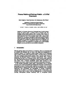
A. Construction of a coarse-grained random walk Start by considering an arbitrary partition {Si }1≤i≤k of the set of nodes Ω. Our aim is to aggregate the points in each set in order to coarse-grain both the state set Ω and the time evolution of the random e whose weight walk. To do so, we regard each set Si as corresponding to the nodes of a k-node graph G, function is defined as XX φ0 (x)pt (x, y) , w(S e i , Sj ) = x∈Si y∈Sj

where the sum involves all the transition probabilities between points x ∈ Si and y ∈ Sj (see Figure 1). S1

o o

~ ,S ) w(S 1 2

o

w(x,y)

S2

o

o

o S1

o o

o

Coarse−graining

o o o

o

o

S3

o

o S2

o S3 o

o

Fig. 1. Example of a coarse-graining of a graph: For a given partition Ω = S1 ∪ S2 ∪ S3 of the set of nodes in a graph G, we define e by aggregating all nodes belonging to a subset Si into a meta-node. By appropriately averaging the transition a coarse-grained graph G probabilities between points x ∈ Si and y ∈ Sj , for i, j = 1, 2, 3, we then compute new weights w(S e i , Sj ) and a new Markov chain with transition probabilities pe(Si , Sj ).

From the reversibility condition of Equation 2, it can be verified that this graph is symmetric, i.e. that w(S e i , Sj ) = w(S e j , Si ). By setting X φe0 (Si ) = φ0 (x) , x∈Si

one can define a reversible Markov chain on this graph with stationary distribution φe0 ∈ Rk and transition probabilities X X φ0 (x) w(S e i , Sj ) pe(Si , Sj ) = P = pt (x, y) . e i , Sk ) φe0 (Si ) k w(S x∈Si y∈Sj

Let Pe be the k × k transition matrix on the coarse-grained graph. More generally, for 0 ≤ l ≤ n − 1, we define in a similar way coarse-grained versions of φl by summing over the nodes in a partition: X φel (Si ) = φl (x) . (10) x∈Si

As in Equation 4, we define coarse-grained versions of ψl according to the duality condition φel (Si ) , ψel (Si ) = φe0 (Si ) which is equivalent to taking a weighted average of ψl over Si : X φ0 (x) ψel (Si ) = ψl (x) . e x∈Si φ0 (Si )

(11)

(12)

8

The coarse-grained kernel pe(Si , Sj ) contains all the information in the data regarding the connectivity e The extent to which the above vectors constitute approximations of the of the new nodes in the graph G. left and right eigenvectors of Pe depends on the particular choice of the partition {Si }. We investigate this issue more precisely in the next section. B. Approximation error. Definition of geometric centroids In a similar manner to Equation 5 and Equation 6, we define the norm on coarse-grained signed measures φel to be X φe2 (Si ) l kφel k21/φe0 = , φe0 (Si ) i

and on the coarse-grained test functions ψel to be X kψel k2φe0 = ψel2 (Si )φe0 (Si ) . i

We now introduce the definition of a geometric centroid, or a representative point, of each partition Si : Definition 1 (geometric centroid): Let 1 ≤ i ≤ k. The geometric centroid c(Si ) of subset Si of Ω is defined as the weighted sum X φ0 (x) c(Si ) = Ψt (x) . e x∈Si φ0 (Si ) The following result shows that for small values of l, φel and ψel are approximate left and right eigenvectors of Pe with eigenvalue λtl . Theorem 2: We have for 0 ≤ l ≤ n − 1, φeTl Pe = λtl φeTl + el and Peψel = λtl ψel + fl . where

kel k21/φe0 ≤ 2D and kfl k2φe0 ≤ 2D ,

and

XX

D=

i

√

φ0 (x)kΨt (x) − c(Si ))k2

x∈Si

This means that if |λl | À D then φel and ψel are approximate left and right eigenvectors of Pe with approximate eigenvalue λtl . The proof of this theorem can be found in Appendix . The previous result also shows that in order to maximize the quality of approximation, we need to minimize the following distortion in diffusion space: XX φ0 (x)kΨt (x) − c(Si ))k2 (13) D = t

i

≈ Ei

x∈Si

©

© ªª EX|i kΨt (X) − c(Si ))k2 |X ∈ Si ,

which can also be written in terms of a weighted sum of pairwise distances according to X X φ0 (x) φ0 (z) 1Xe φ0 (Si ) kΨt (x) − Ψt (z)k2 D = e e 2 i z∈Si x∈Si φ0 (Si ) φ0 (Si ) © © ªª 1 ≈ Ei EX,Z|i kΨt (X) − Ψt (Z))k2 |X, Z ∈ Si . 2

(14)

9

C. An algorithm for distortion minimization Finally, we make a connection to kernel k-means and the algorithmic aspects of the minimization. The form of D given in Equation 13 is classical in information theory, and its minimization is equivalent to solving the problem of quantizing the diffusion space with k codewords based on the mass distribution of the sample set Ψt (Ω). This optimization issue is often addressed via the k-means algorithm [16] which guarantees convergence towards a local minimum: (0) 1) Step 0: initialize the partition {Si }1≤i≤k at random in the diffusion space, 2) For p > 0, update the partition according to (p)

Si

(p−1)

= {x such that i = arg min kΨt (x) − c(Sj j

(p−1)

)k2 } ,

(p−1)

where 1 ≤ i ≤ k, and c(Sj ) is the geometric centroid of Sj , 3) Repeat point 2 until convergence. A drawback of this approach is that each center of mass {c(Si )} may not belong to the set Ψt (E) itself. This can be a problem in some applications where such combinations have no meaning, such as in the case of gene data. In order to obtain representatives {ci } of the clusters that belong to the original set E, we introduce the following definition of diffusion centers: Definition 3 (diffusion center): The diffusion center u(S) of a subset S of Ω is any solution of arg min kΨt (x) − c(S)k2 . x∈Ω This notion does not define a unique diffusion center, but it is sufficient for our purpose of minimizing the distortion. Note that u(S) is a generalization of the idea of center of mass to graphs. Now, if {Si } is the output of the k-means algorithm, then we can assign to each point in Si the e is a subsampled version of G that, for a given value representative center u(Si ). In that sense, the graph G of k, retains the spectral properties of the graph. The analysis above provides a rigorous justification for k-means clustering in diffusion spaces, and furthermore links our work to both spectral graph partitioning (where often only the first non-trivial eigenvector of the graph Laplacian is taken into account) and eigenmaps (where one uses spectral coordinates for data parameterization). IV. N UMERICAL EXAMPLES A. Importance of learning the nonlinear geometry of data in clustering In many applications, real data sets exhibit highly nonlinear structures. In such cases, linear methods such as Principal Components will not be very efficient for representing the data. With the diffusion coordinates, however, it is possible to learn the intrinsic geometry of data set, and then project the data points into a non-linear coordinate space with a diffusion metric. In this diffusion space, one can use classical geometric algorithms (such as separating hyperplane-based methods, k-means algorithms, etc.) for unsupervised as well as supervised learning. To illustrate this idea, we study the famous Swiss roll. This data set is intrinsically a surface embedded in 3 dimensions. In this original coordinate system, global extrinsic distances, such as the Euclidean distance, are often meaningless as they do not incorporate any information on the structure or shape of the data set. For instance, if we run the k-means algorithm for clustering with k = 4, the obtained clusters do not reflect the natural geometry of the set. As shown in Figure 2, there is some “leakage” between different parts of the spiral due to the convexity of the k-means clusters in the ambient space. As a comparison, we also show in Figure 2 the result of running the k-means algorithm in diffusion space. In the latter case, we obtain meaningful clusters that respect the intrinsic geometry of the data set.

10

3 2 1

3 2 1

−1.5 1

−1

−1.5 1

−1

−0.5 0

0

−0.5 0

0

0.5 −1

Fig. 2.

1

0.5 −1

1

The Swiss roll, and its quantization by k-means (k = 4) in the original coordinate system (left) and in the diffusion space (right).

B. Robustness of the diffusion distance One of the most attractive features of the diffusion distance is its robustness to noise and small perturbations of the data. In short, its stability follows from the fact that it reflects the connectivity of the points in the graph. We illustrate this idea by studying the case of data points approximately lying on a spiral in the two-dimensional plane. The goal of this experiment is to show that the diffusion distance is a robust metric on the data, and in order to do so, we compare it to the shortest path (or geodesic) distance that is employed in schemes such as ISOMAP [13]. We generate 1000 instances of a noisy spiral in the plane, each corresponding to a different realization of the random noise perturbation (see Figure 3). From each instance, we construct a graph by connecting all pairs of points at a distance less than a given threshold τ , which is kept constant over the different realizations of the spiral. The corresponding adjacency matrix W contains only zeros or ones, depending on the absence or presence of an edge, respectively. In order to measure the robustness of the diffusion distance, we repeatedly compute the diffusion distance between two points of reference A and B in all 1000 noisy spirals. We also compute the geodesic distance between these two points using Dijkstra’s algorithm. As shown in Figure 3, depending on the presence of shortcuts arising from points appearing between the branches of the spiral, the geodesic distance (or shortest path length) between A and B may vary by large amounts from one realization of the noise to another. The histogram of all geodesic distances measurements between A and B over the 1000 trials is shown on Figure 4. The distribution of the geodesic distance appears poorly localized, as its standard deviation equals 42% of its mean. This indicates that the geodesic distance is extremely sensitive to noise and thus unreliable as a measure of distance. The diffusion distance, however, is not sensitive to small random perturbations of the data set because, unlike the geodesic distance, it represents an average quantity. More specifically, it takes into account all paths of length less than or equal to t that connect A and B. As a consequence, shortcuts due to noise will have little weight in the computation, as the number of such paths is much smaller than the number of paths following the shape of the spiral. This is also what our experiment confirms: Figure 4 shows the distribution of the diffusion distances between A and B over the random trials. In this experiment, t was taken to be equal to 600. The corresponding histogram shows a very localized distribution, with a standard deviation equal to only 7% of its mean, which translates into robustness and consistency of the diffusion distance.

11

1.2

1

1 0.8

0.8

B

0.6

0.6

0.4

0.4

0.2

0.2

0

0

A

−0.2

−0.2

−0.4

−0.4

−0.6

−0.6

−0.8

−1

−0.5

0

B

0.5

1

−0.8

A

−1

−0.5

0

0.5

1

Fig. 3. Two realizations of a noisy spiral with points of references A and B. Ideally, the shortest path between A and B should follow the branch of the spiral (left). However, some realizations of the noise may give rise to shortcuts, thereby dramatically reducing the length of the shortest path (right).

C. Organizing and clustering words via diffusion maps Many of the ideas in this paper can be illustrated with an application to word-document clustering. We here show how we can measure the semantic association of words using diffusion distances, and how we can organize and form representative meta-words using diffusion maps and the k-means algorithm. Our starting point is a collection of p = 1161 Science News articles. These articles belong to 8 different categories (see [17]). Our goal is to cluster words based on their distribution over the documents. From the database, we extract the 20 most common words in each document, which corresponds to 3218 unique words total. Out of these words, we then select words with an intermediate documentPconditional entropy. The conditional entropy of a document X given a word y is defined as HX|y = − x p(x|y) log p(x|y). Words with a very low entropy occur, by definition, in few documents and are often not good descriptors of the database, while high-entropy words such as “it”, “if”, “and”, etc. can be equally uninformative. Thus, in our case, we choose a set of N = 1004 words with entropy 2 < H(X|y) < 4. As in [17], we calculate the mutual information between document x and word y according to à ! fx, y P mx, y = log P , ξ fξ, y η fξ,η where fx,y = cx,y /N , and cx,y is the number of times word w appears in document x. In the analysis below, we describe word y in terms of the p-dimensional feature vector ey = [m1, y , m2, y , . . . mp, y ] . Our first task is to find a low-dimensional embedding of the words. We form the kernel µ ¶ ||ei − ej ||2 w(ei , ej ) = exp − , σ2 and normalize it, as described in Section II-A, to obtain the diffusion kernel pt (ei , ej ). We then embed the data using the eigenvalues λtk and the eigenvectors ψk of the kernel (see Equation 8). As mentioned, the effective dimensionality of the embedding is given by the spectral fall-off of the eigenvalues. For σ = 18 and t = 4, we have that (λ10 /λ1 )t < 0.1, which means that we have effectively reduced the dimensionality

12

Geodesic distance 100

50

0

0

0.5

1

1.5

2

1.5

2

Diffusion distance

100

50

0

Fig. 4. to 1.

0

0.5

1

Distribution of the geodesic (top) and diffusion (bottom) distances. Each distribution was rescaled in order to have a mean equal

Diffusion center psychiatric talent laser velocity gravitational orbiting geologic warming underwater ecosystem farmer virus cholesterol

All other words in cluster depression, psychiatrist, psychologist award, competition, finalist, intel, prize, scholarship, student, winner beam, nanometer, photon, pulse, quantum detector, emit, infrared, ultraviolet bang, cosmo, gravity, hubble jupiter, orbit, solar beneath, crust, depth, earthquake, ice, km, plate, seismic, trapped, volcanic climate, el, nino, pacific, weather atlantic, coast, continent, floor, island, marine, seafloor, sediment algae, drought, dry, ecologist, extinction, forest, gulf, lake, pollution, river carolina, crop, fish, florida, insect, nutrient, pesticide, pollutant, soil, tree, tropical, wash, wood aids, allergy, hiv, resistant, vaccine, viral aging, artery, fda, insulin, obesity, sugar, vitamin TABLE II

E XAMPLES OF DIFFUSION CENTERS AND WORDS IN A CLUSTER

of the original p-dimensional problem, where p = 1161, with a factor of about 1/100. Figure 5 shows the first two coordinates in the diffusion map; Euclidean distances in the figure only approximately reflect diffusion distances since higher-order coordinates are not displayed. Note that the words have roughly been rearranged according to their semantics. Starting to the left, moving counter-clockwise, we have words that, respectively, express concepts in medicine, social sciences, computer science, physics, astronomy, earth sciences and anthropology. Next, we show that the original 1004 words can be clustered and grouped into representative “metawords” by minimizing the distortion in Equation 13. The k-means algorithm with k = 100 cluster leads to the results in Figure 5. Table II furthermore gives some examples of diffusion centers and words in a cluster. The diffusion centers or “meta-words” form a coarse-grained representation of the word graph and can, for example, be used as conceptual indices for document retrieval and document clustering. This will be discussed in later work.

13

−6

x 10 6

4

fossil warming specimen africa

t

λ2 ψ2

2

0

−2

underwater

geologic ecosystem oceanographer wind noaa dioxide antarctica farmerextinct reef debris sankvent crater bird spill hydrothermal sprayed skeletal whale mosquito craft prairie hunting taste herd germ foam stamp sticky pilecopper wright yeast ala tape count longevity committee tolerance screening cruz embryonic smoke pitch sex viruse consciousness zhang symbol cholesterol carroll simulation spinal syndrome efficacy alpha facial plasma magnetic vacuum glow companion infectious liver surgery ii player interference dust voltage collision emotion tumor adulthood secret entrymusic velocity computation microwave laser circuitequation boy quasar medication psychiatric sixth expansion gravitational

orbiting

galaxy

talent

telescope

−4

−4

−2

0

2

4 t λ1

ψ1

6

8

10 −6

x 10

Fig. 5. Embedding and k-means clustering of 1004 words for t = 4 and k = 100. The colors correspond to the different word clusters, and the text labels the representative diffusion center or “meta-word” of each word cluster. Note that the words are automatically arranged according to their semantics.

V. D ISCUSSION In this work, we provide evidence that clustering, graph partitioning and data set parametrization can be solved within one and the same framework. Our starting point is to find a meaningful representation of the data, and to explicitly define a distance metric on the data. Here we propose using a system of coordinates and a metric that reflects the connectivity of the data set. By doing so, we lay down a solid foundation for subsequent data analysis. All the geometry of the data set is captured in a diffusion kernel. However, unlike SVM and so called “kernel methods” [18], [19], [20], we are working with the embedding coordinates explicitly. Our method is completely data driven: both the data representation and the kernel are computed directly on the data. The notion of a distance allows us to more precisely define our goals in clustering and dimensionality reduction. In addition, the diffusion framework makes it possible to directly connect grouping in embedding spaces to spectral graph clustering and data analysis by Markov chains [21], [11]. In a sense, we are extending Meila and Shi’s work [3] from lumpable Markov chains and piece-wise constant eigenvectors to the general case of arbitrary Markov chains and arbitrary eigenvectors. The key idea is to work with embedding spaces directly and also to take powers of the transition matrix. The time

14

parameter t sets the scale of the analysis. Note also that by using different values of t, we are able to perform a multiscale analysis of the data [22], [23]. Our other contribution is a novel scheme for simultaneous dimensionality reduction, parameterization and subsampling of data sets. We show that clustering in embedding spaces is equivalent to compressing operators. As mentioned, the diffusion operator defines the geometry of our data set. There are several ways of compressing a linear operator, depending on what properties one wishes to retain. For instance, in [22], the goal is to maintain sparseness of the representation while achieving the best compression rate. On the other hand, the objective in our work is to cluster or partition a given data set while at the same time preserving the operator (that captures the geometry of the data set) up to some accuracy. We show that, for a given partitioning scheme, the corresponding quantization distortion in diffusion space bounds the error of compression of the operator. This gives us a precise measure of the performance of clustering algorithms. To find the best clustering, one needs to minimize this distortion, and the k-means algorithm is one way to achieve this goal. Another aspect of our approach is that we are coarse-graining a Markov chain defined on the data, thus offering a general scheme to subsample and parameterize graphs based on intrinsic geometry. ACKNOWLEDGMENTS We are grateful to R.R. Coifman for his insight and guidance. We would also like to thank M. Maggioni and B. Nadler for contributing in the development of the diffusion framework, and Y. Keller for providing comments on the manuscript. A PPENDIX In this section, we provide a proof for Theorem 2, which we recall as Theorem 4: We have for 0 ≤ l ≤ n − 1, φeT Pe = λt φeT + el and Peψel = λt ψel + fl . l l

l

where

l

kel k21/φe0 ≤ 2D and kfl k2φe0 ≤ 2D ,

and D=

XX i

√

φ0 (x)kΨt (x) − c(Si ))k2

x∈Si

This means that if |λl | À D then φel and ψel are approximate left and right eigenvectors of Pe with approximate eigenvalue λtl . Proof: We start by treating left eigenvectors: For all z ∈ Si , we define t

rij (z) = pe(Si , Sj ) − pt (z, Sj ) . Then

¯ ¯ ¯ X φ (x) ¯ ¯ ¯ 0 |rij (z)| = ¯ (pt (x, Sj ) − pt (z, Sj ))¯ e ¯ ¯ x∈Si φ0 (Si ) X φ0 (x) X ≤ |pt (x, y) − pt (z, y)| e x∈Si φ0 (Si ) y∈Sj  12   12  X φ0 (x) X X 1  |pt (x, y) − pt (z, y)|2  (Cauchy-Schwarz) ≤ φ0 (y)  e φ (y) 0 x∈S φ0 (Si ) y∈S y∈S i

j

j

 21 q X φ0 (x) X 1  φe0 (Sj ) |pt (x, y) − pt (z, y)|2  ≤ e φ0 (y) x∈Si φ0 (Si ) y∈Sj 

15

Another application of the Cauchy-Schwarz inequality yields X φ0 (x) X 1 |pt (x, y) − pt (z, y)|2 |rij (z)|2 ≤ φe0 (Sj ) e φ (y) 0 x∈Si φ0 (Si ) y∈Sj Thus,

X

φel (Si )e p(Si , Sj ) =

i

=

XX i

z∈Si

i

z∈Si

XX

φl (z)e p(Si , Sj ) φl (z)(pt (z, Sj ) + rij (z))

= λtl φel (Sj ) +

XX i

We therefore define el ∈ Rk by el (Sj ) =

XX i

φl (z)rij (z)

z∈Si

φl (z)rij (z) .

z∈Si

To prove the theorem, we need to bound kel k21/φe0 =

X el (Sj )2 j

φe0 (Sj )

.

First, observe that by the Cauchy-Schwartz inequality, !Ã ! Ã XX X X φl (z)2 rij (z)2 φ0 (z) . el (Sj )2 ≤ φ (z) 0 i z∈S i z∈S i

i

Now, since φl was normalized, this means that ! Ã XX rij (z)2 φ0 (z) . el (Sj )2 ≤ i

z∈Si

Invoking inequality (15), we conclude that XXX X φ0 (x) X 1 kel k21/φe0 ≤ φ0 (z) |pt (x, y) − pt (z, y)|2 e φ (y) 0 j i z∈Si x∈Si φ0 (Si ) y∈Sj XX X φ0 (x) X 1 ≤ φ0 (z) |pt (x, y) − pt (z, y)|2 e φ0 (y) i z∈Si x∈Si φ0 (Si ) y X X X φ0 (x) φ0 (z) Dt2 (x, z) ≤ φe0 (Si ) e e i z∈Si x∈Si φ0 (Si ) φ0 (Si ) X X X φ0 (x) φ0 (z) ≤ φe0 (Si ) kΨt (x) − Ψt (z)k2 e e i z∈Si x∈Si φ0 (Si ) φ0 (Si ) X X X φ0 (x) φ0 (z) ≤ φe0 (Si ) e e i z∈Si x∈Si φ0 (Si ) φ0 (Si ) ×(kΨt (x) − c(Si )k2 + kΨt (z) − c(Si )k2 − 2hΨt (x) − c(Si ), Ψt (z) − c(Si )i) By definition of c(Si ), X X φ0 (x) φ0 (z) hΨt (x) − c(Si ), Ψt (z) − c(Si )i = 0 , φe0 (Si ) φe0 (Si )

z∈Si x∈Si

(15)

16

and therefore

kel k21/φe0 ≤ 2

XX i

φ0 (x)kΨt (z) − c(Si )k2 .

x∈Si

As for right eigenvectors, the result follows from Equation 11 and the fact that the coarse-grained Markov chain is reversible with respect to φe0 . Indeed, X Peψel (Si ) = pe(Si , Sj )ψel (Sj ) j

=

X pe(Si , Sj ) j

=

φ0 (Sj )

X pe(Sj , Si ) j

φ0 (Si )

φel (Sj ) by Equation 11 φel (Sj ) by reversibility

φel (Si ) el (Si ) + φe0 (Si ) φe0 (Si ) el (Si ) = λtl ψel (Si ) + by Equation 11. φe0 (Si ) = λtl

If we set fl (Si ) = el (Si )/φe0 (Si ), we conclude that X el (Si )2 kfl k2φe0 = φe (S ) = kel k21/φe0 ≤ 2D . e0 (Si )2 0 i φ i

R EFERENCES [1] Y. Weiss. Segmentation using eigenvectors: a unifying view. In Proceedings IEEE International Conference on Computer Vision, volume 14, pages 975–982, 1999. [2] J. Shi and J. Malik. Normalized cuts and image segmentation. IEEE Tran PAMI, 22(8):888–905, 2000. [3] M. Meila and J. Shi. A random walk’s view of spectral segmentation. AI and Statistics (AISTATS), 2001. [4] S.T. Roweis and L.K. Saul. Nonlinear dimensionality reduction by locally linear embedding. Science, 290:2323–2326, 2000. [5] Z. Zhang and H. Zha. Principal manifolds and nonlinear dimension reduction via local tangent space alignement. Technical Report CSE-02-019, Department of computer science and engineering, Pennsylvania State University, 2002. [6] M. Belkin and P. Niyogi. Laplacian eigenmaps for dimensionality reduction and data representation. Neural Computation, 6(15):1373– 1396, June 2003. [7] D.L. Donoho and C. Grimes. Hessian eigenmaps: new locally linear embedding techniques for high-dimensional data. Proceedings of the National Academy of Sciences, 100(10):5591–5596, May 2003. [8] F. Chung. Spectral graph theory. Number 92. CBMS-AMS, May 1997. [9] R.R. Coifman and S. Lafon. Diffusion maps. Applied and Computational Harmonic Analysis, 2006. To appear. [10] R.R. Coifman, S. Lafon, A.B. Lee, M. Maggioni, B. Nadler, F. Warner, and S. Zucker. Geometric diffusions as a tool for harmonics analysis and structure definition of data: Diffusion maps. Proceedings of the National Academy of Sciences, 102(21):7426–7431, 2005. [11] M. Szummer and T. Jaakkola. Partially labeled classification with markov random walks. In Advances in Neural Information Processing Systems, volume 14, 2001. [12] I.S. Dhillon, Y. Guan, and B. Kulis. Kernel k-means, spectral clustering and normalized cuts. Proceedings of The Tenth ACM SIGKDD International Conference on Knowledge Discovery and Data Mining(KDD), 2004. [13] V. de Silva J.B. Tenenbaum and J.C. Langford. A global geometric framework for nonlinear dimensionality reduction. Science, 290:2319–2323, 2000. [14] B. Nadler, S. Lafon, R.R. Coifman, and I. Kevrekidis. Diffusion maps, spectral clustering and the reaction coordinates of dynamical systems. Applied and Computational Harmonic Analysis, 2006. To appear. [15] Private communication with R.R. Coifman. [16] S. Lloyd. Least squares quantization in pcm. IEEE Transactions on Information Theory, 28(2):129–138, 1982. [17] C.E. Priebe, D.J. Marchette, Y. Park, E.J. Wegman, J.L. Solka, D.A. Socolinsky, D. Karakos, K.W. Church, R. Guglielmi, R.R. Coifman, D. Lin, D.M. Healy, M.Q. Jacobs, and A. Tsao. Iterative denoising for cross-corpus discovery. In Proceedings IEEE International Conference on Computer Vision pp. 975–982., 2004. [18] B. Schölkopf, A.J. Smola, and K.-R. Müller. Nonlinear component analysis as a kernel eigenvalue problem. Neural Computation, 10(5):1299–1319, 1998.

17

[19] V.N. Vapnik. The nature of statistical learning theory. 2nd edition. [20] C.J.C. Burges. A tutorial on support vector machines for pattern recognition. Data mining and knowledge discovery, 2:121–167, 1998. [21] F. Fouss, A. Pirotte, J.-M. Renders, and M. Saerens (2004). A novel way of computing similarities between nodes of a graph, with application to collaborative recommendation. 2004. submitted to publication. [22] R.R. Coifman and M. Maggioni. Diffusion wavelets. Applied and Computational Harmonic Analysis, 2006. To appear. [23] R.R. Coifman, S. Lafon, A.B. Lee, M. Maggioni, B. Nadler, F. Warner, and S. Zucker. Geometric diffusions as a tool for harmonics analysis and structure definition of data: Multiscale methods. Proceedings of the National Academy of Sciences, 102(21):7432–7437, 2005.

Stéphane Lafon is a Software Engineer at Google. He received his B.Sc. degree in Computer Science from Ecole Polytechnique and his M.Sc. in Mathematics and Artificial Intelligence from Ecole Normale Supérieure de Cachan in France. He obtained his Ph.D. in Applied Mathematics at Yale University in 2004 and he was a Research Associate in the Applied Mathematics group during the year 2004-2005. He is currently with Google where his work focuses on the design, analysis and implementation of machine learning algorithms. His research interests are in data mining, machine learning and information retrieval.

Ann B. Lee is an Assistant Professor of Statistics at Carnegie Mellon University. She received her M.Sc. degree in Engineering Physics from Chalmers University of Technology in Sweden, and her Ph.D. degree in Physics from Brown University in 2002. She was a Research Associate in the Division of Applied Mathematics (Pattern Theory Group) at Brown University during the year 2001-2002, and a J.W. Gibbs Instructor and Assistant Professor of Applied Mathematics at Yale University from 2002-2005. In August 2005, she joined the Department of Statistics at Carnegie Mellon. Her research interests are in machine learning, statistical models in pattern analysis and vision, high-dimensional data analysis and multi-scale geometric methods.