Jul 13, 2006 - Hessian eigenmaps [7], LTSA [5], and diffusion maps [9],. [10], all aim ...... For more information on th
IEEE TRANSACTIONS ON PATTERN ANALYSIS AND MACHINE INTELLIGENCE,
VOL. 28, NO. 9,
SEPTEMBER 2006
1393
Diffusion Maps and Coarse-Graining: A Unified Framework for Dimensionality Reduction, Graph Partitioning, and ! 0 are discussed in [9]. The graph G with weights W represents our knowledge of the local geometry of the set. Next, we define a Markov random walk on this graph. To this end, we introduce the degree dðxÞ of node x as X dðxÞ ¼ wðx; zÞ: z2�
If one defines P to be the n � n matrix whose entries are given by
p1 ðx; yÞ ¼
1395
wðx; yÞ ; dðxÞ
then p1 ðx; yÞ can be interpreted as the probability of transition from x to y in one time step. By construction, this quantity reflects the first-order neighborhood structure of the graph. A new idea introduced in the diffusion maps framework is to capture information on larger neighborhoods by taking powers of the matrix P or, equivalently, to run the random walk forward in time. If P t is the tth iterate of P , then the entry pt ðx; yÞ represents the probability of going from x to y in t time steps. Increasing t, corresponds to propagating the local influence of each node with its neighbors. In other words, the quantity P t reflects the intrinsic geometry of the data set defined via the connectivity of the graph in a diffusion process and the time t of the diffusion plays the role of a scale parameter in the analysis. If the graph is connected, we have that [8]: lim pt ðx; yÞ ¼ �0 ðyÞ;
ð1Þ
t!þ1
where �0 is the unique stationary distribution dðxÞ : z2� dðzÞ
�0 ðxÞ ¼ P
This quantity is proportional to the degree of x in the graph, which is one measure of the density of points. The Markov chain is furthermore reversible, i.e., it verifies the following detailed balance condition �0 ðxÞp1 ðx; yÞ ¼ �0 ðyÞp1 ðy; xÞ:
ð2Þ
We are mainly concerned with the following idea: For a fixed but finite value t > 0, we want to define a metric between points of � which is such that two points x and z will be close if the corresponding conditional distributions pt ðx; :Þ and pt ðz; :Þ are close. A similar idea appears in [11], where the authors consider the L1 norm jjpt ðx; :Þ � pt ðz; :Þjj. Alternatively, one can use the Kullback-Leibler divergence or any other distance between pt ðx; :Þ and pt ðz; :Þ. However, as shown below, the L2 metric between the conditional distributions has the advantage that it allows one to relate distances to the spectral properties of the random walk —and thereby, as we will see in the next section, connect Markov random walk learning on graphs with data parameterization via eigenmaps. As in [14], we will define the “diffusion distance” Dt between x and y as the weighted L2 distance D2t ðx; zÞ ¼ kpt ðx; �Þ � pt ðz; �Þk21=�0 ¼
X ðpt ðx; yÞ � pt ðz; yÞÞ2 y2�
�0 ðyÞ
;
ð3Þ 1 �0 ðxÞ
where the “weights” penalize discrepancies on domains of low density more than those of high density. This notion of proximity of points in the graph reflects the intrinsic geometry of the set in terms of connectivity of the data points in a diffusion process. The diffusion distance between two points will be small if they are connected by many paths in the graph. This metric is thus a key quantity in the design of inference algorithms that are based on the preponderance of evidences for a given hypothesis. For example, suppose one wants to infer class labels for data points based on a small number of labeled examples. Then, one can easily propagate the label information from a labeled
1396
IEEE TRANSACTIONS ON PATTERN ANALYSIS AND MACHINE INTELLIGENCE,
example x to the new point y following 1) the shortest path or 2) all paths connecting x to y. The second solution (which is employed in the diffusion framework and in [11]) is usually more appropriate, as it takes into account all “evidences” relating x to y. Furthermore, since diffusion-based distances add up the contribution from several paths, they are also (unlike the shortest path) robust to noise; the latter point is illustrated via an example in Section 4.2.
2.2
Dimensionality Reduction and Parameterization of Data by Diffusion Maps As mentioned, an advantage of the above definition of the diffusion distance is the connection to the spectral theory of the random walk. As is well-known, the transition matrix P that we have constructed has a set of left and right eigenvectors and a set of eigenvalues j�0 j � j�1 j � . . . � j�n�1 j: �Tj P ¼ �j �Tj and P
j
¼ �j
j;
where it can be verified that �0 ¼ 1, 0 � 1, and that �Tk l ¼ �kl . In fact, left and right eigenvectors are dual and can be regarded as signed measures and test functions, respectively. These two sets of vectors are related according to l ðxÞ ¼
�l ðxÞ for all x 2 �: �0 ðxÞ
ð4Þ
For ease of notation, we normalize the left eigenvectors of P with respect to 1=�0 : X �2 ðxÞ
k�l k21=�0 ¼
l
x
�0 ðxÞ
¼ 1;
ð5Þ
and the right eigenvectors with respect to the weight �0 : X 2 ð6Þ k l k2�0 ¼ l ðxÞ�0 ðxÞ ¼ 1: x
If pt ðx; yÞ is the kernel of the tth iterate P t , we will then have the following biorthogonal spectral decomposition: X pt ðx; yÞ ¼ �tj j ðxÞ�j ðyÞ: ð7Þ
VOL. 28,
NO. 9,
SEPTEMBER 2006
accuracy. To be precise, let qðtÞ be the largest index j such that j�j jt > �j�1 jt . The diffusion distance can then be approximated to relative precision � using the first qðtÞ nontrivial eigenvectors and eigenvalues according to D2t ðx; zÞ ’
qðtÞ X
�2t j ð j ðxÞ �
j ðzÞÞ
2
:
j¼1
Now, observe that the identity above can be interpreted as the Euclidean distance in IRqðtÞ if we use the right eigenvectors weighted with �tj as coordinates on the data. In other words, this means that, if we introduce the diffusion map 0 t 1 �1 1 ðxÞ B �t2 2 ðxÞ C B C ð8Þ �t : x 7�!B .. C; @ A . �tqðtÞ qðtÞ ðxÞ then clearly, D2t ðx; zÞ ’
qðtÞ X
�2t j ð j ðxÞ �
j ðzÞÞ
2
¼ k�t ðxÞ � �t ðzÞk2 : ð9Þ
j¼1
Note that the factors �tj in the definition of �t are crucial for this statement to hold. The mapping �t : � ! IRqðtÞ provides a parameterization of the data set �, or equivalently, a realization of the graph G as a cloud of points in a lower-dimensional space IRqðtÞ , where the rescaled eigenvectors are the coordinates. The dimensionality reduction and the weighting of the relevant eigenvectors are dictated by both the time t of the random walk and the spectral fall-off of the eigenvalues. Equation (9) means that �t embeds the entire data set in IRqðtÞ in such a way that the Euclidean distance is an approximation of the diffusion distance. Our approach is thus different from other eigenmap methods: Our starting points is an explicitly defined distance metric on the data set or graph. This distance is also the quantity we wish to preserve during a nonlinear dimensionality reduction.
j�0
The above identity corresponds to a weighted principal component analysis of P t . The first k terms provide the best rank-k approximation of P t , where “best” is defined according to the following weighted metric for matrices: kAk2 ¼
XX x
�0 ðxÞaðx; yÞ2
y
1 : �0 ðyÞ
Here is our main point: If we insert (7) into (3), we will have that D2t ðx; zÞ ¼
n�1 X
�2t j ð j ðxÞ �
2 j ðzÞÞ :
j¼1
Since 0 � 1 is a constant vector, it does not enter in the sum above. Furthermore, because of the decay of the eigenvalues,1 we only need a few terms in the sum for a certain 1. The speed of the decay depends on the graph structure. For example, for the special case of a fully connected graph, the first eigenvalue will be 1 and the remaining eigenvalues will be equal to 0. The other extreme case is a graph that is totally disconnected with all eigenvalues equal to 1.
3
GRAPH PARTITIONING
AND
SUBSAMPLING
In what follows, we describe a novel scheme for subsampling data sets that—as above—preserves the intrinsic geometry defined by the connectivity of the data points in a graph. The idea is to construct a coarse-grained version of the original e with similar spectral random walk on a new graph G properties. This new Markov chain is obtained by grouping points into clusters and appropriately averaging the transition probabilities between these clusters. We show that in order to retain most of the spectral properties of the original random walk, the choice of clusters in critical. More precisely, the quantization distortion in diffusion space bounds the error of the approximation of the diffusion operator. One application is dimensionality reduction and clustering of arbitrarily shaped data sets using geometry; see Section 4 for some simple examples. However, more generally, the construction also offers a systematic way of subsampling operators [15] and arbitrary graphs using geometry.
LAFON AND LEE: DIFFUSION MAPS AND COARSE-GRAINING: A UNIFIED FRAMEWORK FOR DIMENSIONALITY REDUCTION, GRAPH...
1397
e The extent to which the above new nodes in the graph G. vectors constitute approximations of the left and right eigenvectors of Pe depends on the particular choice of the partition fSi g. We investigate this issue more precisely in the next section.
3.2
Approximation Error: Definition of Geometric Centroids In a similar manner to (5) and (6), we define the norm on coarse-grained signed measures �el to be
Fig. 1. Example of a coarse-graining of a graph: For a given partition � ¼ S1 [ S2 [ S3 of the set of nodes in a graph G, we define a coarsee by aggregating all nodes belonging to a subset Si into a grained graph G metanode. By appropriately averaging the transition probabilities between points x 2 Si and y 2 Sj , for i; j ¼ 1; 2; 3, we then compute new weights e i ; Sj Þ and a new Markov chain with transition probabilities peðSi ; Sj Þ. wðS
3.1 Construction of a Coarse-Grained Random Walk Start by considering an arbitrary partition fSi g1�i�k of the set of nodes �. Our aim is to aggregate the points in each set in order to coarse-grain both the state set � and the time evolution of the random walk. To do so, we regard each set e Si as corresponding to the nodes of a k-node graph G, whose weight function is defined as XX e i ; Sj Þ ¼ wðS �0 ðxÞpt ðx; yÞ; x2Si y2Sj
where the sum involves all the transition probabilities between points x 2 Si and y 2 Sj (see Fig. 1). From the reversibility condition of (2), it can be verified e j ; Si Þ. e i ; Sj Þ ¼ wðS that this graph is symmetric, i.e., that wðS By setting X �0 ðxÞ; �e0 ðSi Þ ¼
k�el k2 e ¼ 1=�0
l ; �e0 ðSi Þ and on the coarse-grained test functions el to be X e2 ðSi Þ�e0 ðSi Þ: k el k2e ¼ l �0
We now introduce the definition of a geometric centroid, or a representative point, of each partition Si : Definition 1 (Geometric Centroid). Let 1 � i � k. The geometric centroid cðSi Þ of subset Si of � is defined as the weighted sum cðSi Þ ¼
i
j
Let Pe be the k � k transition matrix on the coarse-grained graph. More generally, for 0 � l � n � 1, we define in a similar way coarse-grained versions of �l by summing over the nodes in a partition: X �l ðxÞ: ð10Þ �el ðSi Þ ¼ x2Si
As in (4), we define coarse-grained versions of to the duality condition
l
e el ðSi Þ ¼ �l ðSi Þ ; e �0 ðSi Þ which is equivalent to taking a weighted average of
The following result shows that for small values of l, �el and el are approximate left and right eigenvectors of Pe with eigenvalue �tl . Theorem 1. We have for 0 � l � n � 1, �eTl Pe ¼ �tl �eTl þ el and Pe el ¼ �tl el þ fl ; where kel k2 e � 2D and kfl k2e � 2D; �0 1=�0
X �0 ðxÞ el ðSi Þ ¼ e x2S �0 ðSi Þ
and D¼
l over Si :
i
ð12Þ
i
The coarse-grained kernel peðSi ; Sj Þ contains all the information in the data regarding the connectivity of the
�0 ðxÞk�t ðxÞ � cðSi ÞÞk2 :
x2Si
x2Si
n n oo Ei EXji k�t ðXÞ � cðSi ÞÞk2 jX 2 Si ;
ð13Þ
where E represents an expectation. This can also be written in terms of a weighted sum of pairwise distances according to X X �0 ðxÞ �0 ðzÞ 1X e k�t ðxÞ � �t ðzÞk2 �0 ðSi Þ e e 2 i z2Si x2Si �0 ðSi Þ �0 ðSi Þ n oo 1 n Ei EX;Zji k�t ðXÞ � �t ðZÞÞk2 jX; Z 2 Si : 2 ð14Þ
D¼ l ðxÞ:
XX
pffiffiffiffi This means that, if j�l jt � D, then �el and el are approximate left and right eigenvectors of Pe with approximate eigenvalue �tl . The proof of this theorem can be found in the Appendix. The previous result also shows that, in order to maximize the quality of approximation, we need to minimize the following distortion in diffusion space: XX D¼ �0 ðxÞk�t ðxÞ � cðSi ÞÞk2
according
ð11Þ
X �0 ðxÞ �t ðxÞ: e x2S �0 ðSi Þ i
i
X X �0 ðxÞ wðS e i ; Sj Þ pt ðx; yÞ: peðSi ; Sj Þ ¼ P ¼ e i ; Sk Þ x2S y2S �e0 ðSi Þ k wðS
i
i
x2Si
one can define a reversible Markov chain on this graph with stationary distribution �e0 2 IRk and transition probabilities
X �e2 ðSi Þ
1398
IEEE TRANSACTIONS ON PATTERN ANALYSIS AND MACHINE INTELLIGENCE,
VOL. 28,
NO. 9,
SEPTEMBER 2006
Fig. 2. The Swiss roll, and its quantization by k-means (k ¼ 4) in the (a) original coordinate system and in the (b) diffusion space.
3.3 An Algorithm for Distortion Minimization Finally, we make a connection to kernel k-means and the algorithmic aspects of the minimization. The form of D given in (13) is classical in information theory and its minimization is equivalent to solving the problem of quantizing the diffusion space with k codewords based on the mass distribution of the sample set �t ð�Þ. This optimization issue is often addressed via the k-means algorithm [16] which guarantees convergence toward a local minimum: 1. 2.
ð0Þ
Step 0: initialize the partition fSi g1�i�k at random in the diffusion space. For p > 0, update the partition according to � � ðpÞ ðp�1Þ 2 Þk ; Si ¼ x such that i ¼ arg min k�t ðxÞ � cðSj j
ðp�1Þ k and cðSj Þ is the geometric centroid
where 1 � i � ðp�1Þ of Sj . 3. Repeat point 2 until convergence. A drawback of this approach is that each center of mass fcðSi Þg may not belong to the set �t ðEÞ itself. This can be a problem in some applications where such combinations have no meaning, such as in the case of gene data. In order to obtain representatives fci g of the clusters that belong to the original set E, we introduce the following definition of diffusion centers: Definition 2 (Diffusion Center). The diffusion center uðSÞ of a subset S of � is any solution of arg min k�t ðxÞ � cðSÞk2 : x2�
This notion does not define a unique diffusion center, but it is sufficient for our purpose of minimizing the distortion. Note that uðSÞ is a generalization of the idea of center of mass to graphs. Now, if fSi g is the output of the k-means algorithm, then we can assign to each point in Si the representative center e is a subsampled version of uðSi Þ. In that sense, the graph G G that, for a given value of k, retains the spectral properties of the graph. The analysis above provides a rigorous justification for k-means clustering in diffusion spaces, and furthermore links our work to both spectral graph partitioning
(where often only the first nontrivial eigenvector of the graph Laplacian is taken into account) and eigenmaps (where one uses spectral coordinates for data parameterization).
4
NUMERICAL EXAMPLES
4.1
Importance of Learning the Nonlinear Geometry of Data in Clustering In many applications, real data sets exhibit highly nonlinear structures. In such cases, linear methods such as Principal Components will not be very efficient for representing the data. With the diffusion coordinates, however, it is possible to learn the intrinsic geometry of data set and then project the data points into a nonlinear coordinate space with a diffusion metric. In this diffusion space, one can use classical geometric algorithms (such as separating hyperplane-based methods, k-means algorithms, etc.) for unsupervised as well as supervised learning. To illustrate this idea, we study the famous Swiss roll. This data set is intrinsically a surface embedded in three dimensions. In this original coordinate system, global extrinsic distances, such as the Euclidean distance, are often meaningless as they do not incorporate any information on the structure or shape of the data set. For instance, if we run the k-means algorithm for clustering with k ¼ 4, the obtained clusters do not reflect the natural geometry of the set. As shown in Fig. 2, there is some “leakage” between different parts of the spiral due to the convexity of the k-means clusters in the ambient space. As a comparison, we also show in Fig. 2 the result of running the k-means algorithm in diffusion space. In the latter case, we obtain meaningful clusters that respect the intrinsic geometry of the data set. 4.2 Robustness of the Diffusion Distance One of the most attractive features of the diffusion distance is its robustness to noise and small perturbations of the data. In short, its stability follows from the fact that it reflects the connectivity of the points in the graph. We illustrate this idea by studying the case of data points approximately lying on a spiral in the two-dimensional plane. The goal of this experiment is to show that the diffusion distance is a robust metric on the data, and in order to do so, we compare it to the
LAFON AND LEE: DIFFUSION MAPS AND COARSE-GRAINING: A UNIFIED FRAMEWORK FOR DIMENSIONALITY REDUCTION, GRAPH...
1399
Fig. 3. Two realizations of a noisy spiral with points of references A and B. Ideally, the shortest path between A and B should follow the (a) branch of the spiral. However, some realizations of the noise may give rise to shortcuts, thereby dramatically reducing the length of the (b) shortest path.
shortest path (or geodesic) distance that is employed in schemes such as ISOMAP [13]. We generate 1,000 instances of a noisy spiral in the plane, each corresponding to a different realization of the random noise perturbation (see Fig. 3). From each instance, we construct a graph by connecting all pairs of points at a distance less than a given threshold �, which is kept constant over the different realizations of the spiral. The corresponding adjacency matrix W contains only zeros or ones, depending on the absence or presence of an edge, respectively. In order to measure the robustness of the diffusion distance, we repeatedly compute the diffusion distance between two points of reference A and B in all 1,000 noisy spirals. We also compute the geodesic distance between these two points using Dijkstra’s algorithm. As shown in Fig. 3, depending on the presence of shortcuts arising from points appearing between the branches of the spiral, the geodesic distance (or shortest path length) between A and B may vary by large amounts from one realization of the noise to another. The histogram of all geodesic distances measurements between A and B over the 1,000 trials is shown on Fig. 4. The distribution of the geodesic distance appears poorly localized, as its standard deviation equals 42 percent of its mean. This indicates that the geodesic distance is extremely sensitive to noise and thus unreliable as a measure of distance. The diffusion distance, however, is not sensitive to small random perturbations of the data set because, unlike the geodesic distance, it represents an average quantity. More specifically, it takes into account all paths of length less than or equal to t that connect A and B. As a consequence, shortcuts due to noise will have little weight in the computation, as the number of such paths is much smaller than the number of paths following the shape of the spiral. This is also what our experiment confirms: Fig. 4 shows the distribution of the diffusion distances between A and B over the random trials. In this experiment, t was taken to be equal to 600. The corresponding histogram shows a very localized distribution, with a standard deviation equal to only 7 percent of its mean, which translates into robustness and consistency of the diffusion distance.
4.3
Organizing and Clustering Words via Diffusion Maps Many of the ideas in this paper can be illustrated with an application to word-document clustering. We here show how we can measure the semantic association of words using diffusion distances and how we can organize and form representative metawords using diffusion maps and the k-means algorithm. Our starting point is a collection of p ¼ 1; 161 Science News articles. These articles belong to eight different categories (see [17]). Our goal is to cluster words based on their distribution over the documents. From the database, we extract the 20 most common words in each document, which corresponds to 3,218 unique words total. Out of these words, we then select words with an intermediate document conditional entropy. The conditional entropy of a document
Fig. 4. Distribution of the (a) geodesic and (b) diffusion distances. Each distribution was rescaled in order to have a mean equal to 1.
1400
IEEE TRANSACTIONS ON PATTERN ANALYSIS AND MACHINE INTELLIGENCE,
VOL. 28,
NO. 9,
SEPTEMBER 2006
Fig. 5. Embedding and k-means clustering of 1,004 words for t ¼ 4 and k ¼ 100. The colors correspond to the different word clusters, and the text labels the representative diffusion center or “metaword” of each word cluster. Note that the words are automatically arranged according to their semantics.
P X given a word y is defined as HXjy ¼ � x pðxjyÞ log pðxjyÞ. Words with a very low entropy occur, by definition, in few documents and are often not good descriptors of the database, while high-entropy words such as “it,” “if,” “and,” etc. can be equally uninformative. Thus, in our case, we choose a set of N ¼ 1; 004 words with entropy 2 < H ðXjyÞ < 4. As in [17], we calculate the mutual information between document x and word y according to ! fx; y P mx; y ¼ log P ; � f�; y � f�;� where fx;y ¼ cx;y =N and cx;y is the number of times word w appears in document x. In the analysis below, we describe word y in terms of the p-dimensional feature vector ey ¼ ½m1; y ; m2; y ; . . . mp; y : Our first task is to find a low-dimensional embedding of the words. We form the kernel ! jjei � ej jj2 wðei ; ej Þ ¼ exp � ; �2 and normalize it, as described in Section 2.1, to obtain the diffusion kernel pt ðei ; ej Þ. We then embed the data using the
eigenvalues �tk and the eigenvectors k of the kernel (see (8)). As mentioned, the effective dimensionality of the embedding is given by the spectral fall-off of the eigenvalues. For � ¼ 18 and t ¼ 4, we have that ð�10 =�1 Þt < 0:1, which means that we have effectively reduced the dimensionality of the original p-dimensional problem, where p ¼ 1; 161, with a factor of about 1=100. Fig. 5 shows the first two coordinates in the diffusion map; Euclidean distances in the figure only approximately reflect diffusion distances since higher-order coordinates are not displayed. Note that the words have roughly been rearranged according to their semantics. Starting to the left, moving counterclockwise, we have words that, respectively, express concepts in medicine, social sciences, computer science, physics, astronomy, earth sciences, and anthropology. Next, we show that the original 1; 004 words can be clustered and grouped into representative “metawords” by minimizing the distortion in (13). The k-means algorithm with k ¼ 100 cluster leads to the results in Fig. 5. Table 2 furthermore gives some examples of diffusion centers and words in a cluster. The diffusion centers or “metanode” form a coarse-grained representation of the word graph and can, for example, be used as conceptual indices for document retrieval and document clustering. This will be discussed in later work.
LAFON AND LEE: DIFFUSION MAPS AND COARSE-GRAINING: A UNIFIED FRAMEWORK FOR DIMENSIONALITY REDUCTION, GRAPH...
1401
TABLE 2 Examples of Diffusion Centers and Words in a Cluster
5
DISCUSSION
In this work, we provide evidence that clustering, graph partitioning, and data set parameterization can be solved within one and the same framework. Our starting point is to find a meaningful representation of the data and to explicitly define a distance metric on the data. Here, we propose using a system of coordinates and a metric that reflects the connectivity of the data set. By doing so, we lay down a solid foundation for subsequent data analysis. All the geometry of the data set is captured in a diffusion kernel. However, unlike SVM and so-called “kernel methods” [18], [19], [20], we are working with the embedding coordinates explicitly. Our method is completely data driven: Both the data representation and the kernel are computed directly on the data. The notion of a distance allows us to more precisely define our goals in clustering and dimensionality reduction. In addition, the diffusion framework makes it possible to directly connect grouping in embedding spaces to spectral graph clustering and data analysis by Markov chains [21], [11]. In a sense, we are extending Meila and Shi’s work [3] from lumpable Markov chains and piece-wise constant eigenvectors to the general case of arbitrary Markov chains and arbitrary eigenvectors. The key idea is to work with embedding spaces directly and also to take powers of the transition matrix. The time parameter t sets the scale of the analysis. Note also that by using different values of t, we are able to perform a multiscale analysis of the data [22], [23]. Our other contribution is a novel scheme for simultaneous dimensionality reduction, parameterization, and subsampling of data sets. We show that clustering in embedding spaces is equivalent to compressing operators. As mentioned, the diffusion operator defines the geometry of our data set.
There are several ways of compressing a linear operator, depending on what properties one wishes to retain. For instance, in [22], the goal is to maintain sparseness of the representation while achieving the best compression rate. On the other hand, the objective in our work is to cluster or partition a given data set while at the same time preserving the operator (that captures the geometry of the data set) up to some accuracy. We show that, for a given partitioning scheme, the corresponding quantization distortion in diffusion space bounds the error of compression of the operator. This gives us a precise measure of the performance of clustering algorithms. To find the best clustering, one needs to minimize this distortion, and the k-means algorithm is one way to achieve this goal. Another aspect of our approach is that we are coarse-graining a Markov chain defined on the data, thus offering a general scheme to subsample and parameterize graphs based on intrinsic geometry.
APPENDIX In this section, we provide a proof for Theorem 1, which we recall as Theorem 2. We have for 0 � l � n � 1, �eTl Pe ¼ �tl �eTl þ el and Pe el ¼ �tl el þ fl ; where kel k2 e � 2D and kfl k2e � 2D; 1=�0 �0 and D¼
XX i
x2Si
�0 ðxÞk�t ðxÞ � cðSi ÞÞk2 :
1402
IEEE TRANSACTIONS ON PATTERN ANALYSIS AND MACHINE INTELLIGENCE,
pffiffiffiffi This means that, if j�l jt � D, then �el and el are approximate left and right eigenvectors of Pe with approximate eigenvalue �tl . Proof. We start by treating left eigenvectors: For all z 2 Si , we define
kel k2 e � 1=�0
�
112
�
!12 1 2 ðCauchy-SchwarzÞ jpt ðx; yÞ � pt ðz; yÞj � ðyÞ y2Sj 0 0 112 qffiffiffiffiffiffiffiffiffiffiffiffiffiffi X X � ðxÞ 1 0 @ � �e0 ðSj Þ jpt ðx; yÞ�pt ðz; yÞj2A : e � ðyÞ 0 ðS Þ � 0 i x2S y2S j
Another application of the Cauchy-Schwarz inequality yields X �0 ðxÞ X 1 jpt ðx; yÞ � pt ðz; yÞj2 : e � ðyÞ 0 � ðS Þ 0 i x2S y2S j
ð15Þ
pðSi ; Sj Þ ¼ �el ðSi Þe
i
XX i
¼
XX
�l ðzÞe pðSi ; Sj Þ
j
i
i
i
X X �0 ðxÞ �0 ðzÞ �e0 ðSi Þ e e z2S x2S �0 ðSi Þ �0 ðSi Þ i
i
� 2h�t ðxÞ � cðSi Þ; �t ðzÞ � cðSi ÞiÞ: By definition of cðSi Þ, X X �0 ðxÞ �0 ðzÞ h�t ðxÞ � cðSi Þ; �t ðzÞ � cðSi Þi ¼ 0; e e z2S x2S �0 ðSi Þ �0 ðSi Þ i
i
and, therefore, kel k2 e � 2 1=�0
z2Si
þ
XX
¼
j
¼
�0 ðSj Þ
X peðSj ; Si Þ j
We therefore define el 2 IRk by XX el ðSj Þ ¼ �l ðzÞrij ðzÞ:
¼ �tl
�0 ðSi Þ
�el ðSj Þ by ð11Þ �el ðSj Þ by reversibility
�el ðSi Þ el ðSi Þ þ �e0 ðSi Þ �e0 ðSi Þ
¼ �tl el ðSi Þ þ
z2Si
X el ðSj Þ
x2Si
j
�l ðzÞrij ðzÞ:
To prove the theorem, we need to bound
i
�0 ðxÞk�t ðzÞ � cðSi Þk2 :
X peðSi ; Sj Þ
z2Si
i
XX
As for right eigenvectors, the result follows from (11) and the fact that the coarse-grained Markov chain is reversible with respect to �e0 . Indeed, X peðSi ; Sj Þ el ðSj Þ Pe el ðSi Þ ¼
�l ðzÞðpt ðz; Sj Þ þ rij ðzÞÞ
�tl �el ðSj Þ
i
i
X X �0 ðxÞ �0 ðzÞ k�t ðxÞ � �t ðzÞk2 �e0 ðSi Þ e e z2S x2S �0 ðSi Þ �0 ðSi Þ
z2Si
i
¼
X i
X
Thus, X
z2Si
� ðk�t ðxÞ � cðSi Þk2 þ k�t ðzÞ � cðSi Þk2
j
i
X i
j
X �0 ðxÞ X @ �0 ðyÞA � e x2S �0 ðSi Þ y2S
jrij ðzÞj2 � �e0 ðSj Þ
i
X �0 ðxÞ X 1 jpt ðx; yÞ e � ðyÞ x2S �0 ðSi Þ y2S 0
i
X �0 ðxÞ X jpt ðx; yÞ � pt ðz; yÞj e x2S �0 ðSi Þ y2S
i
j
�0 ðzÞ
� pt ðz; yÞj2 X X X �0 ðxÞ �0 ðzÞ D2t ðx; zÞ � �e0 ðSi Þ e e ðS Þ ðS Þ � � 0 i i z2S x2S 0 i
i
i
XXX
� pt ðz; yÞj XX X �0 ðxÞ X 1 � �0 ðzÞ jpt ðx; yÞ e �0 ðyÞ i z2Si x2Si �0 ðSi Þ y
� � � X � ðxÞ � � � 0 ðpt ðx; Sj Þ � pt ðz; Sj ÞÞ� jrij ðzÞj ¼ � �x2S �e0 ðSi Þ �
0
SEPTEMBER 2006
2
Then,
i
NO. 9,
Invoking (15), we conclude that
rij ðzÞ ¼ peðSi ; Sj Þ � pt ðz; Sj Þ:
�
VOL. 28,
el ðSi Þ by ð11Þ: e �0 ðSi Þ
If we set fl ðSi Þ ¼ el ðSi Þ=�e0 ðSi Þ, we conclude that
2
kel k2 e ¼ 1=�0
j
�e0 ðSj Þ
:
�0
First, observe that by the Cauchy-Schwartz inequality, ! ! XX X X �l ðzÞ2 2 2 el ðSj Þ � rij ðzÞ �0 ðzÞ : �0 ðzÞ i z2S i z2S i
i
Now, since �l was normalized, this means that ! XX 2 2 rij ðzÞ �0 ðzÞ : el ðSj Þ � i
z2Si
kfl k2e ¼
X el ðSi Þ2 �e ðS Þ ¼ kel k2 e � 2D: 2 0 i 1=�0 e i �0 ðSi Þ t u
ACKNOWLEDGMENTS The authors would like to thank R.R. Coifman for his insight and guidance, M. Maggioni and B. Nadler for contributing in the development of the diffusion framework, and Y. Keller for providing comments on the manuscript.
LAFON AND LEE: DIFFUSION MAPS AND COARSE-GRAINING: A UNIFIED FRAMEWORK FOR DIMENSIONALITY REDUCTION, GRAPH...
REFERENCES [1] [2] [3] [4] [5]
[6] [7] [8] [9] [10]
[11] [12] [13] [14]
[15] [16] [17]
[18] [19] [20] [21]
[22] [23]
Y. Weiss, “Segmentation Using Eigenvectors: A Unifying View,” Proc. IEEE Int’l Conf. Computer Vision, vol. 14, pp. 975-982, 1999. J. Shi and J. Malik, “Normalized Cuts and Image Segmentation,” IEEE Trans. Pattern Analysis and Machine Intelligence, vol. 22, no. 8, pp. 888-905, Aug. 2000. M. Meila and J. Shi, “A Random Walk’s View of Spectral Segmentation,” AI and Statistics (AISTATS), 2001. S.T. Roweis and L.K. Saul, “Nonlinear Dimensionality Reduction by Locally Linear Embedding,” Science, vol. 290, pp. 2323-2326, 2000. Z. Zhang and H. Zha, “Principal Manifolds and Nonlinear Dimension Reduction via Local Tangent Space Alignement,” Technical Report CSE-02-019, Dept. of Computer Science and Eng., Pennsylvania State Univ., 2002. M. Belkin and P. Niyogi, “Laplacian Eigenmaps for Dimensionality Reduction and Data Representation,” Neural Computation, vol. 6, no. 15, pp. 1373-1396, June 2003. D.L. Donoho and C. Grimes, “Hessian Eigenmaps: New Locally Linear Embedding Techniques for High-Dimensional Data,” Proc. Nat’l Academy of Sciences, vol. 100, no. 10, pp. 5591-5596, May 2003. F. Chung, Spectral Graph Theory, no. 92, CBMS-AMS, May 1997. R.R. Coifman and S. Lafon, “Diffusion Maps,” Applied and Computational Harmonic Analysis, to appear. R.R. Coifman, S. Lafon, A.B. Lee, M. Maggioni, B. Nadler, F. Warner, and S. Zucker, “Geometric Diffusions as a Tool for Harmonics Analysis and Structure Definition of Data: Diffusion Maps,” Proc. Nat’l Academy of Sciences, vol. 102, no. 21, pp. 74267431, 2005. M. Szummer and T. Jaakkola, “Partially Labeled Classification with Markov Random Walks,” Advances in Neural Information Processing Systems, vol. 14, 2001. I.S. Dhillon, Y. Guan, and B. Kulis, “Kernel K-Means, Spectral Clustering and Normalized Cuts,” Proc. 10th ACM SIGKDD Int’l Conf. Knowledge Discovery and Data Mining, 2004. V. de Silva, J.B. Tenenbaum, and J.C. Langford, “A Global Geometric Framework for Nonlinear Dimensionality Reduction,” Science, vol. 290, pp. 2319-2323, 2000. B. Nadler, S. Lafon, R.R. Coifman, and I. Kevrekidis, “Diffusion Maps, Spectral Clustering and the Reaction Coordinates of Dynamical Systems,” Applied and Computational Harmonic Analysis, to appear. Private communication with R.R. Coifman. S. Lloyd, “Least Squares Quantization in PCM,” IEEE Trans. Information Theory, vol. 28, no. 2, pp. 129-138, 1982. C.E. Priebe, D.J. Marchette, Y. Park, E.J. Wegman, J.L. Solka, D.A. Socolinsky, D. Karakos, K.W. Church, R. Guglielmi, R.R. Coifman, D. Lin, D.M. Healy, M.Q. Jacobs, and A. Tsao, “Iterative Denoising for Cross-Corpus Discovery,” Proc. IEEE Int’l Conf. Computer Vision, pp. 975-982, 2004. B. Scho¨lkopf, A.J. Smola, and K.-R. Mu¨ller, “Nonlinear Component Analysis as a Kernel Eigenvalue Problem,” Neural Computation, vol. 10, no. 5, pp. 1299-1319, 1998. V.N. Vapnik, The Nature of Statistical Learning Theory, second ed. 1995. C.J.C. Burges, “A Tutorial on Support Vector Machines for Pattern Recognition,” Data Mining and Knowledge Discovery, vol. 2, pp. 121167, 1998. F. Fouss, A. Pirotte, J.-M. Renders, and M. Saerens, “A Novel Way of Computing Similarities between Nodes of a Graph, with Application to Collaborative Recommendation,” Web Intelligence, 2005. R.R. Coifman and M. Maggioni, “Diffusion Wavelets,” Applied and Computational Harmonic Analysis, to appear. R.R. Coifman, S. Lafon, A.B. Lee, M. Maggioni, B. Nadler, F. Warner, and S. Zucker, “Geometric Diffusions as a Tool for Harmonics Analysis and Structure Definition of Data: Multiscale Methods,” Proc. Nat’l Academy of Sciences, vol. 102, no. 21, pp. 7432-7437, 2005.
1403
Ste´phane Lafon received the BSc degree in computer science from Ecole Polytechnique and the MSc degree in mathematics and artificial intelligence from Ecole Normale Supe´rieure de Cachan in France. He received the PhD degree in applied mathematics at Yale University in 2004 and was a research associate in the Applied Mathematics Group during the year 2004-2005. He is currently with Google where he works as a software engineer and his work focuses on the design, analysis, and implementation of machine learning algorithms. His research interests are in data mining, machine learning, and information retrieval. Ann B. Lee received the MSc degree in engineering physics from Chalmers University of Technology in Sweden, and the PhD degree in physics from Brown University in 2002. She is an assistant professor of statistics at Carnegie Mellon University. She was a research associate in the Division of Applied Mathematics (Pattern Theory Group) at Brown University during the year 2001-2002, and a J.W. Gibbs Instructor and assistant professor of applied mathematics at Yale University from 2002-2005. In August 2005, she joined the Department of Statistics at Carnegie Mellon as an assistant professor of statistics. Her research interests are in machine learning, statistical models in pattern analysis and vision, high-dimensional data analysis, and multiscale geometric methods.
. For more information on this or any other computing topic, please visit our Digital Library at www.computer.org/publications/dlib.