Digital fuzzy logic controller: design and implementation - IEEE Xplore

IEEE TRANSACTIONS ON FUZZY SYSTEMS, VOL. 4, NO. 4, NOVEMBER 1996

439

Digital Fuzzy Logic Controller: Design and Implementation Marek J. Patyra, Member, IEEE, Janos L. Grantner, Senior Member, IEEE, and Kirby Koster, Associate Member, IEEE

Abstract-In this paper, various aspects of digital fuzzy logic laid down. Second, the set of major characteristics is defined controller (FLC) design and implementation are discussed. followed by the analytical formulation of single-input singleClassic and improved models of the single-input single-output output (SISO), multiple-input single-output (MISO), and (SISO), multiple-input single-output (MISO), and multiple-input multiple-output (MIMO) FLC’s are analyzed in terms of multiple-input multiple-output (MIMO) FLC models. Third, hardware cost and performance. A set of universal parameters the very large scale integration (VLSI) implementation issues to characterize any hardware realization of digital FLC’s is are discussed and are illustrated with a MIMO FLC design. defined. The comparative study of classic and alternative MIMO Finally, the summary concludes this paper. FLC’s is presented as a generalization of other controller configurations. A processing element (PE) for the parallel FLC architecture realizing improved inferencing of MIMO system is 11. FUZZY LOGICHARDWARE designed, characterized, and tested. Finally, as a case feasibility This section reviews some basic concepts behind the digstudy, a direct data stream (DDS) architecture for complete digital fuzzy controller is shown as an improved solution for ital hardware implementations of fuzzy logic circuits. It is, high-speed, cost-effective, real-time control applications. therefore, an introduction to FLC implementations analyzed

I. INTRODUCTION

T

HIS paper discusses the most important design issues for digital fuzzy logic control circuits. Digital fuzzy logic controllers (FLC) are so far the most commercially successful implementations of fuzzy logic circuits. The dominant position of digital fuzzy logic control circuits can be explained considering psychological, economical, and technical factors. Since the development of the first functional inference engine by Togai and Watanabe in 1985 [52]-[54], there have been many successful developments of digital implementations of fuzzy logic-based systems published to date (see, for example, [4]-[16], [18]-[27], [32]-[35], and [38]-[61]). Due to the wide variety of such achievements, it is hard to appropriately characterize and compare various FLC devices. This is often confusing when different data are provided, especially in terms of overall FLC performance, compatibility, and capability. Hence, the purpose of this paper is twofold. First, it is to present the unified theoretical background for fuzzy logic controllers and their classic and improved models, as well as to discuss FLC implementations in terms of hardware cost and performance. Second, it is to illustrate the improved implementation of highly parallel FLC in digital technique. Interval-based membership functions and/or fuzzy operators are not considered 1551. The organization of this paper is the following. First, the general foundation regarding digital fuzzy logic control is Manuscript received May 17, 1995; revised February 26, 1996. M. J. Patyra and K. Koster are with the Department of Electrical and Computer Engineering, University of Minnesota, Duluth, MN 55812 USA. J. L. Grantner is with the Department of Electrical and Computer Engineering, Western Michlgan University, Kalamazoo, MI 49008 USA. Publisher Item Identifier S 1063-6706(96)06584-8.

in Section 111. The theory behind fuzzy control is not outlined in this paper. For theoretical details regarding the fuzzy logic control and fuzzy logic controllers, the reader is referred to the introductory and tutorial papers [30], [31], and [62], or recently published books [7] and [22]. Most of the control applications of fuzzy logic can be generalized by means of a simple structure shown in Fig. 1. Let us briefly discuss the main stages of the control scheme delineated in Fig. 1. A. Fuzzijication

Fuzzification is a transformation of the crisp data into a corresponding fuzzy set. Before the data can be fuzzified, however, it should first be normalized to meet the range of the universe of discourse suitable for the controller input. The normalization unit is not shown in Fig. 1. Typically, the state of the process is examined by means of its parameter measurements. Such measurements generate the analog-type data available for further use in control system. Assume that the analog output from the process under control is feedback to the digital fuzzy controller. First, the analogto-digital conversion has to be performed followed by the input-data normalization. Note that both procedures mentioned above have their own accuracy and resolution. This fact suggests some fuzzification techniques that can compensate for the unavoidable loss of accuracy. It is important to stress that these procedures are usually responsible for introduction of a systematic error to the input data. As a result, the fuzzification can follow three basic strategies. 1) An input crisp data is converted into a fuzzy singleton in an appropriate universe of discourse. Precisely, the

1063-6706/96$05.00 0 1996 IEEE

440


Fig. 1. The general scheme of the fuzzy logic-based control

fuzzy singleton is a crisp value and, hence, no fuzziness is introduced to the input data; but this strategy has been widely used for fuzzy control applications because of its computational simplicity. 2) An input crisp data is converted into a fuzzy vector based on expert knowledge of the characteristics of measurement instruments, A/Dconversion, and normalization. In this case, all “vagueness” associated with the measurement and transformations are included in the resulting fuzzy vector. 3 ) An input crisp data is randomly distributed and, therefore, can be converted into fuzzy vector with arbitrary shape. However, the distribution of the fuzzy vector may be determined by the parameters of the probability distribution available for the specific measurement process. Fig. 2 illustrates the example of an arbitrary, experimentally, measured variable A; its value is normalized, quantized, and finally discretized into a fuzzy set A. The variable A value measured at the continuous universe of discourse can be represented by an arbitrary singleton, triangle, or any other function as listed above. Note that the discrete universe of discourse is discretized into n’ equal intervals. The degree of membership is also quantized into m’ levels. This membership function is digitized as shown by the step-shape function. As a result, the membership function is represented by a set of perpendicular segments. The digitized representation of the input variable is transformed into a Boolean matrix that has the size of n*m,where n denotes the number of m-bit binary vectors. Each vector is obtained from the digitized membership function in such a way that the m-bit number codes the degree of membership function on the appropriate position defined by n’ segment. Note that if 2“ # m’, the mapping must be nonlinear. Also, in practice n may not be equal to n’, which creates the additional problem of horizontal nonlinear mapping from universe of discourse discretized into n’ intervals into n vectors. B. Fuzzy Inference To discuss fuzzy inferencing in great detail, let us recall the fuzzy system characterized by the linguistic description in the

Measured Value A

-

....

Continuous .---Universe of Discourse

Normalization Quantization Discretization

’uzzy Set A

Discretized 1 /n’

Universe of Discourse

Cent& Value Binary Mapping

m

0 0 Fig. 2.

Binary Mamx

n

Example illustrating the idea and steps of fuzzification process

form of fuzzy implication rules

RI:IF A 1 IS A: AND IF A2 IS A: AND . . . AND IF AK IS AF THEN B1 IS B: AND B2 IS B: AND . . . AND B L IS Bf ALSO

PATYRA

et

al.: DIGITAL FUZZY LOGIC CONTROLLER

Rz: IF A1 IS Ai AND IF A2 IS A: AND . . . AND IF A K IS A 5 THEN B 1 IS Bi AND B2 IS BZ AND ALSO

AND B L IS B i

R;: IF A1 IS A i AND IF A2 IS A: AND ... AND IF A K IS A: THEN B1 IS Bi AND B2 IS B: AND . . . AND B L IS Bf ALSO R N : IF A1 IS A h AND IF A2 IS A& AND . . . AND IF AK IS A$ THEN B 1 IS B h AND B2 IS B& AND . . . AND B L IS B h

441

the inferred fuzzy output. Sometimes, after the defuzzification, a denormalization procedure is required for practical applications. In terms of digital implementation of a defuzzification strategy, the usual approach involves arithmetic operations on a large number (depending on the granularity of the universe of discourse) of binary vectors. These operations include multiplications, summations, and divisions; therefore, defuzzification is usually one of the most time consuming operation in fuzzy processing. No single optimal defuzzification algorithm exists to date. One may not exist at all, however, the research has been going on to find criteria and methods to switch over from one algorithm to another, or to use some weighted superposition of more that one algorithm with tunable weights. There are numerous defuzzification methods. However, only about five are practical. They are: center-of-area (COA), center-of-gravity (COG), height defuzzification (HD), centerof-largest-area (COLA), and mean-of maxima (MOM). These algorithms are discussed in [44].

CONTROLLERS 111. DIGITALFUZZYLOGIC-BASED represent the input variables, This section discusses hardware implementation issues of A:, A:, . . . , A: represent the input membership functions, B1, ... B K represent the output variables, digital FLC. The section is organized as follows. First, the set and B: B:, . . . BF represent the output membership of major parameters characterizing digital FLC is established. Then, the mathematical background of SISO FLC is discussed. functions. The inference mechanisms employed in fuzzy logic con- Finally, two alternative models for the SISO and the MIMO trollers are generally based on various reasoning schemes. The fuzzy logic controllers are presented. inference result can be obtained using seven different algoA. Digital FLC Characteristics rithms [31]. To define a fuzzy inference refer to [62], however, In this section, a set of major parameters characterizing the practical difficulties arises to implement it. Therefore, some experimental methods that are described in this section are digital fuzzy logic controllers is established based on informareferred to as reasoning algorithms. These methods attempt to tion gathered from the publications referenced in this paper and implement Zadeh’s inference but they are simplified to gain authors experience. We begin our discussion from the general the practical feasibility. Only four fuzzy reasoning methods viewpoint related to the application of FLC devices. There are two basic parameters that determine the usefulness are commonly used. These methods are listed below. 1) Mamdani ’s Strategy-Mamdani’s fuzzy reasoning of a certain implementation of FLC. These are the number of input variables and the number of output variables. In this method is based on MAX-MIN inference operator. case, the usefulness of a FLC can be viewed by means of the 2 ) Larsen’s Strategy-Larsen’ s fuzzy reasoning method is complexity of the process that can be controlled by a FLC based on PRODUCT inference operator. under consideration. 3) Tsukamoto’s Strategy-Tsukamoto’ s fuzzy reasoning Based on the information provided in Section 11, especially method is based on the simplification of Mamdani’s with respect to the fuzzification, inferencing, and defuzzifimethod, although all membership functions (antecedents cation, it has become obvious that the input transformation and conclusions) are monotonic. 4) Takagi and Sugeno ’s Strategy-Takagi and Sugeno’s from the analog measurement to the binary representation of fuzzy reasoning method is based on a distinct model fuzzy information is crucial for the FLC functionality. Also, description. In this model, the control variables are char- the inverse transformation of fuzzy information into a crisp acterized by the functions of the process state variables. output determines the accuracy of the overall control action. On the other hand, in terms of inferencing the basic charFor more elaborative information on these methods, the acteristic of FLC can be referred to as the performance and reader is referred to [30] and [31]. “storage ability.” The latter determines the FLC capacity Inference is performed in the functional block commonly to store linguistic rules as well as the capacity to store known as inference engine. membership functions assigned to different linguistic variable values. C. Defuzzijication One of the major problems of FLC’s characteristics is reGenerally, defuzzification describes the mapping from a lated to their performance. In scientific and technical literature space of fuzzy control action into a nonfuzzy control action. there can be found at least three performance measures. They Defuzzification produces a nonfuzzy action that best represents are:

where

All

.-

AK

IEEE TRANSACTIONS ON FUZZY SYSTFiMS, VOL. 4, NO. 4, NOVEMBER 1996

442

* the maximum frequency of the clock running the FLC

device; the number of fuzzy inferences per second (also called FLIPS) where the fuzzy inference is usually ambiguously defined, or even not defined. The fuzzy inference may be understood as a operation determined by a single rule, or an operation determined be a part of the rule as well; the number of elementary fuzzy operations per second (e.g., MIN or MAX). It has to be stressed that the above parameters do not provide a confident measure of the real speed of the FLC. Therefore, we propose to characterize the FLC be means of the inputto-output delay time (TIN-OUT). Such a time is defined as a total delay time from the moment of providing the input variable to FLC device until the generation of the crisp action at the output of this device.' Such a time is, in our opinion, the most objective measure of the FLC performance because it does take into account the real throughput of the device. The parameters used so far provide, maybe spectacular data, unfortunately these data lack real performance value. Let us take as an example, the FLC device that can perform several million fuzzy logic inferences per second (several MFLIPS), but the control action could be available at the output after, let us say, milliseconds since the input stimulus entered the controller. In such a case, the inference engine of the FLC is mostly occupied with tedious number crunching that do not lead to the final result. As we will present later, such behavior is determined by the internal FLC structure and can be avoided by the appropriate structure modifications to the inference engine made at the design stage. Let us summarize the above discussion and specify the set of major FLC parameters crucial for further discussion. They can be listed as follows: number of input variables (inputs) ( K ) ; number of output variables (outputs) (L); number of linguistic rules in the knowledge base ( N ) ; * number of membership functions in the input universe of discourse (MB,,); * number of membership functions in the output universe of discourse ( M B o u T ) ; ,. number of binary vectors characterizing the membership function (n); number of bits in a single binary vector (m); input-to-output delay time (TIN-OUT). The next sections present the results of an algebraic analysis of various configurations of FLC with regard to the selected parameters. 0

0

C. Multiple-Input Single-Output Fuzzy Logic Controller

1 ) Classic Method: If Ai,Ai, ' , Ah are fuzzy subsets of A', and A:, A;,.. . , A& are fuzzy subsets of A2, and . . ., and Af,A?, . . ' , A 5 are fuzzy subsets of AK; B1,Bz,. . . , BN are fuzzy subsets of B then fuzzy relation R is defined by a set of fuzzy rules as follows: e

RI: IF A: AND IF A: AND.. . AND IF A? THEN B1,ALSO IF Ai AND IF A; AND . . . AND IF R2: A$ THEN Ba, ALSO

R,:

IF At AND IF A: AND . . . AND IF

A :

THEN B,, ALSO

R N : IF Ah AND IF AS AND . . . AND IF AS THEN B N . Observe, that is this case the fuzzy relation is defined by

R = (A1, A', . . . , A K ) + B. If the output B has to be inferred, then according to the definition of fuzzy implication

B = (A', A', . . . , A K )O R .

(1)

Also, using the procedure for building the overall fuzzy relation N

R=

U R,.

(2)

z=1

Having fuzzy observations A l , A2, . . . , AK and the overall relation R, one can infer the resulting action B1 by applying the compositional rule of inference

0

0 0

B1 = ( A l , A2, . . . , A K ) o R N

= ( A I , A2,

. .. , AK) o

U R, z=1

N

=

U ( A l ,A2, . . . , A K ) o R,.

The membership function of B1 can then computed by the well-known MAX-MIN operation. Considering the ith rule R, and the observation A l , the respective action B1 is given by

B1, = ( A l , A2, . . . , A K ) o R,. So the membership function is given by

B. Single-Input Single-Output Fuzzy Logic Controllers The SISO system, as overexploited in the literature, is not discussed in this paper. For details on the analytical description of the SISO FLC, the reader is referred to [52] or [31]. The next section presents analysis of the MIS0 FLC. 'If we consider the pipelined FLC, such device presumably generates the output every clock cycle. In such a case, the clock period determines an input-to-output delay time.

(3)

2=1

P B l , ( b ) =MAxMIN[PAl(al) x

bA2(aZ)

x ".

x P A K ( ~ K ) , ai, a2, U K ,b)l a1 E A l , a2 E A2, . . . , U K E AK )

= MINMAX (MIN {MIN

(4)

443

PATYRA et al.: DIGITAL FTJZZY LOGIC CONTROLLER

The membership function of B1 can then calculated by the well-known MAX-MIN operation. Considering the ith rule R; and the observation Al, the respective action B1 is given by where

is defined by

BZi = (Al, A2, . . . , AK) o R,

(13)

where 1 = 1, 2, ... , L. Therefore, the corresponding membership function is defined as follows:

2 ) Alternative Method: This method is based, by analogy to the previously used technique, on the rule decomposition into subrelations, and building the fuzzy relation first. One can assume that the first and subsequent rules can be decomposed into K separate subrelations as follows:

where i denotes, as usual, the rule number i = 1, 2, . . , N , k denotes the input variable k = 1, 2, . . . , K , and 1 denotes the output variable Z = 1, 2, ... , L. Therefore, if one wants to obtain overall, kth subrule, all contributions have to be unionized

=MIN {MAXMIN [PAl(al), @ A I ,(al)] MAXMIN [PA2(a2) , PAzt (a2)], ’ ‘ . a1 E A l , a2 E A2, . . . , aK E AK, ...

MAXMIN [ P K ( a K ) !PAC ( a K ) ] ) .

N

Rk=

where, in this case, 0, is defined in a different way

U Rf

(9)

i=l

or

-

Then the maximum of BZ1, BZP, , BZN determines the final actions Bl which can be calculated as a union

Rk =MAX[RF(ak, b), R ; ( u ~b), , ... , R b ( a k , b)]. (10)

In this case, the model’s output B1 related to a set of inputs (Al, A2, . . . , A K ) can be obtained using the MINsuperposition of all K relations between the input Ak and the rule R~ B 1 = M I N [ A l 0 R 1 , A 2 o R 2 , ... , A K o R K ] or

B1 =MIN{MAXMIN[Al, Rl(a1, b ) ] , ... MAXMIN [AK, R K ( a ~b)]}. ,

(11)

D. Multiple-tnput Multiple-Output Fuzzy Logic Controller

Let us briefly generalize the results of the discussion of MIS0 FLC to the MIMO controller case. 1 ) Classic Method: Having fuzzy observations A1 and A2, ... , A K and the overall relation R, one can infer the resulting action Bl by applying the compositional rule of inference. As a result B1 = ( A l , A2, ... , A K ) O R N

= (Al, A2,

... , A K ) o U R; i=l

N

=

U ( A l , A2, . . . , A K ) o R;. i=l

(15)

N

BZ =

U BZ,

(16)

i=l

where Z = 1, 2, - . , L denotes the output variable. 2) Alternative Method: By decomposing the relations defined in a single rule, the set of K * L subrelations can be obtained for all N rules. With the same strategy we can define sub-subrelations for each of N rules. In this way, we obtain K * L subrelations that can be used to infer the fuzzy results in case the set of input variables is A1 and A2,... , AK. The model’s outputs can be obtained using MIN-superposition operation through all L relations +

B1 = MIN [(A1 o RI1), (A2 o

. . . , (AK o RK1)] (17)

BL = MIN [(A1 o RIL), (A2 o RZL),. . . , (AK o R K L ) ] . (18) In this way, we can infer all L-fuzzy outputs by the MINsuperposition of all subrules incorporating a respective output variable. More specifically, one can rewrite (17) and (18) into

B1 =MIN{MAXMIN[Al, R”(a1, bi)], ... MAXMIN [AK, RK1(U K , bl)]} BL =MIN{MAXMIN[Al, RlL(al, b ~ ) ]... , MAXMIN [AK, RKL(aK, b ~ ) ] } .

(19) (20)

IEEE TRANSACTIONS ON FUZZY SYSTEMS, VOL. 4, NO 4, NOVEMBER 1996

444

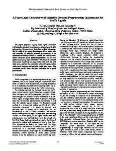
... Fig. 3. Schematic diagram of the MIMO classic FLC.

Summarizing, the altemative method of inference offers two major advantages over the classic one. They are: * compact knowledge base where all rules are accessed simultaneously; * higher sensitivities for the input variables changes. On the other hand, one can point out the disadvantage, which may play role especially with some classes of knowledge-base tuning algorithms, that is, the unavailability of individual rules. Obviously, as practice shows, the ideal algorithm fulfilling all different kinds of requirements is likely not to be found.

E. Hardware Implementation Issues

Hardware implementation of FLC raises several practical difficulties that can be clearly visible by investigating cost functions and overall delays for various hardware configurations. As a general case, we compare implementations of the described MIMO FLC models based on the criteria derived from the set of characteristic parameters. We use the formula parametrized by the following parameters: number of input variableshnputs ( K ) ; number of output variables/outputs ( L ) ; number of linguistic rules in the knowledge base ( N ) ; number of binary vectors characterizing the membership function (n); number of bits in a single binary vector (m). 1) Hardware Characteristics: In the subsequent sections, we analyze only the most general case of FLC implementation: MIMO. The SISO, DISO, or MIS0 can be easily inferred 0 0

0

0

from such analysis by applying simplifying assumptions to the MIMO case. i) MIMO classic implementation: The MIMO FLC model presented in Section 111-D-1, can be mapped into a hardware model in a variety of ways. One of the straightforward ways consists of direct mapping of the inference algorithm into hardware. Observe, that we focus our discussion on the inference engine instead of fuzzifier and defuzzifier. In the subsequent analysis, we assume that the fuzzifier and defuzzifier units have a certain implementation; however, for the purpose of fair comparison of classic and improved FLC implementations they are functionally identical. The block diagram of the classic implementation of the is illustrated in Fig. 3. In case of MIMO FLC, the inference engine is constructed of N MIN units and N MAX units performing the antecedent part of rules for a single input. These pieces of hardware is then multiplied by the number of inputs ( K ) .MIN unit must perform the minimum operation on nm-bit vectors as assumed earlier. Then, the MAX unit determines the maximum value represented by one of these nm-bit vectors. To do the minimum, the antecedent membership functions (representing the values of input linguistic variables) must be stored and ready to enter the MIN units. These functions, as another nm-bit vectors are stored in the rule base memory. Proceeding with fuzzy inference, the consequent membership functions (representing the values of output linguistic variables) are entered into N MIN units along with Nm-bit vectors generated in cumulative MIN units. Cumulative MIN units compute the minimum membership values from all K inputs for a particular rule. These cumulative units are built of N K-input MIN units and they are located between antecedent

PATYRA et al.: DIGITAL FUZZY LOGIC CONTROLLER

445

Fig. 4. Schematic diagram of the MIMO improved FLC.

and consequent parts of the scheme. Consequent membership functions are stored in the rule base memory. Consequent MIN units perform the same type operation as antecedent MIN units. The results of consequent' MIN units are unionized by means of multi-input MAX unit. Such a unit is usually implemented as a MAX unit binary tree, which in this case contains N - 1 MAX units. Finally, the unified defuzzifier generales a crisp output of the FLC,separately for each of L outputs. Taking a MIMO scheme shown in Fig. 3 into consideration one can derive a cost function H as:

process and, therefore, there is no additional delay introduced by the memory-read operation. ii) MIMO alternative implementation: Analyzing the FLC analytical model presented in Section 111-D-2, it is clear that we can map it into a hardware scheme that differs substantially from the schemes proposed to date. One of the possible implementations is illustrated in Fig. 4. As can be noticed from the scheme contained but not shown in Fig. 4,the FLC is mapped into the fuzzifier, inference engine, and defuzzifier as usual. However, we have to point a few distinct differences as opposed to the classic implementation. First of all, in this case learning the overall rule can be done HKNL(C) = KHFUZZ KN(HMAx ~ H M I N ) L(N - ~ ) ~ H M A N(K x - ~ ) H M I N off-line in the part of the scheme contained not shown in Fig. 4. That is a dramatic difference as opposed to classic LNnHMIN KLnmHMEM implementation because a ready-to-use subrule can be stored LHDEFUZZ (21) in the memory. Second, the multiple-MIN unit performing the minimum operation on the overall rule and the incoming fuzzy where: HKNL(C) is a total hardware cost of a FLC with vector can be viewed as (n - 1) ordinary MIN units working K inputs, L outputs, and N rules implemented with classic concurrently. Also, the final MAX unit can be decomposed in is the hardware cost of the fuzzifier unit, method, HFUZZ the same way as a chain of (n - 1) ordinary MAX units. H M I Nis the hardware cost of the basic minimum unit, HMAX If we closely look at the rule learning module, we can notice is the hardware cost of the basic maximum unit, HDEFUZZ is that the process can be implemented with a two MIN units is the and a single MAX unit plus register storing the temporary the hardware cost of the defuzzifier unit, and HMEM hardware cost of the memory cell. result from the MAX unit. Because the learning process can As far as the overall input-to-output delay time is concerned be performed off line, the extensive (parallel) hardware is not (TIN-OUT), the estimation can be derived from the scheme necessary. presented in Fig. 3, by introducing additional delay on the As we see in Fig. 4, the FLC is mapped into the typical multi-input MIN unit. As a result, the following equation can functional blocks. But in this case, the difference is that K be obtained: memory units for each of L output variables have to be provided. TIN-OUT =TFUZZ ~ T M I N (n- ~ ) T M A X (n - ~ ) T M I N As a result, the hardware cost for the improved MIMO FLC (22) controller can be estimated by: (N - MA MAX TDEFUZZ

+

+ +

+

+

+

+

+ +

+

+

+

where TFUZZ is the delay time of the fuzzifier unit, TMIN is the delay time of the basic minimum unit, T M A X is the delay lime of the basic maximum unit, TDEFUZZ is the delay time of the defuzzifier unit; for simplicity, it is assumed that the rulebase memory can be accessed concurrently with the inference

+

HKNL(I) = KHFUZZ K L H M I N n 2 KLnHMAx f KLn2mHMEM K~HMAX ~LHMIN + LHDEFUZZ + KLHREG.

+

+

(23)


446

10*104

8

8*1@

4.2

8 5 a 0

6*1@

2

z

&’

.-b

$

4*104

2*104

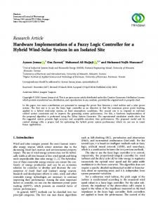
Number of Input Variables (K) Fig. 5. Graphical representation of hardware cost for the classic implementation of FLC. Three surfaces are computed for the following number of rules: N = 10, N = 50, and N = 100.

As far as the overall delay time is concerned, the estimation can be described by the following: TIN-OUT=TFUZZ

+

-t ( K -

+ (n ~)TMAX ~ ) T M I N+ TDEFUZZ.

TMIN

-

(24)

Note that the above result is obtained under the assumption that building the knowledge base is performed off-line. Additionally, the multi-input MIN realization was taken as a worst case (chain of MIN units) and that gives the ( K - ~ ) T M I Nterm. iii) Hardware cost: Comparing the classic and altemative approaches of FLC implementation, in terms of hardware cost we can conclude what follows. Assuming the same cost for the fuzzifier and the defuzzifier modules, the total hardware cost of the classic FLC linearly depends on the number of rules N . Due to its characteristic feature, the improved FLC hardware cost does not depend on the number of rules. The hardware cost for both implementations depends on the number of input and the number of output variables. The hardware cost for both implementations depends on the number of binary vectors characterizing the membership function of the input and the output variables. The hardware cost for both implementations does not depend on the number of membership functions in the input and the output universe of discourses. Let us graphically illustrate the above conclusions. An illustrative comparison of the hardware costs for classic and improved FLC’s is depicted in Fig. 5. In order to fairly compare the hardware cost for both implementations, the following assumptions are made while computing the presented graphs. ,. The MIN and MAX units hardware cost is assumed to be an arbitrary unit. * The fuzzification unit hardware cost is assumed to be ten arbitrary units. The defuzzification unit hardware cost is assumed to be hundred arbitrary units.

For the classic implementation of FLC, the size of fuzzy variable representation is assumed to be n * m = 16 * 4 bits. The 2-y axes represent the number of input variables ( K ) and the number of output variables (L), respectively. Three surfaces are plotted for N = 10, N = 50, and N = 100 rules. The second graph for the classic FLC implementation, delineated in Fig. 6, shows how the representation of the fuzzy number changes the overall hardware cost. Three surfaces plotted in Fig. 6 represent the different binary vector sizes characterizing the membership function: n = 16, n = 32, and n = 64, while m = 4. Also, the number of rules is set to be N = 50. The same strategy is used to illustrate the hardware cost for the improved method of FLC implementation (Fig. 7). The same assumptions hold, however, due to the inherent features, the graph conditions are slightly different. As above, the 2-y axes plane represents the number of input variables ( K )and the number of output variables ( L ) ,respectively. The surfaces are computed for different sizes of fuzzy variable representation: n * m = 16 * 4 bits, n * m = 32 * 8 bits, and n * m = 64 * 16 bits. (As shown earlier, the hardware cost of improved implementation FLC does not depend on the number of rules N ! ) . It is interesting to investigate the hardware costs of both methods of FLC implementation with the similar conditions. The compound graph, delineated in Fig. 8, shows the hardware cost in arbitrary units of the classic FLC and improved FLC. The shown surfaces are computed in such a way that for the classic FLC a typical number of rules is set to N = 100. The surfaces are computed for fuzzy variable representation of the size of n * m = 16 * 4 bits. The z-axis represents the number of input variables K and the y-axis represents the number of output variables L. The last comparison is extremely interesting (see Fig. 8). It shows that for the typical number of rules ( N = loo), the hardware cost of the improved FLC is lower than that of


ln=64

A

of Output !S

1u

20

Q

30

Number of Input Variables (K) Fig. 6. Graphical representation of hardware cost for classic implementation of FLC. Three surfaces arc computed for the following number of binary vectors characterizing the membership function: n = 16, n = 32, and R = 64 ( N = 50).

=64*4 15.104

s" lo*@ Y

r

n*m=32*4

L n*m=16*4 L Numbe Input \

Fig. 7. Graphical representation of hardware cost for the improved implementation of FLC. Three surfaces are computed for fuzzy data matrices o f n * m = 16 4 bits, n * m = 32 * 8 bits, and n * m = 64 * 16 bits.

the classic FLC implementation. Such a conclusion is valid for the improved FLC the hardware cost does not depend on for the number of inputs ranging from zero to approximately the number of rules, and that is what makes this solution even thirty and for the number of outputs ranging from zero to more attractive over the classic one. iv) Pe$ormance: We will compare the performance of approximately fifteen. If the system is more sophisticated the hardware cost of improved FLC grows over that of the classic the two FLC implementations by means of the introduced FLC implementation. However, in most practical applications, overall delay from input to output. Analyzing the formula the number of rules is the key limiting factor for the particular given by (22) and (24), and assuming the same performance FLC implementation.Therefore, we have to keep in mind that of the typical functional units, one can conclude what follows:


448

Improved FLC

T 12.5*1@

g5

10*104 10*104-

U

e!aB 7.5*1047.5*104 3:

.

5*1&

Number of Input Variables (K)

Fig. 8. Graphical comparison of hardware costs for classic and improved implementations of FLC. (The classic FLC is characterized by AT and the fuzzy variable is represented by n * m 2 16 * 4 bits).

zz

100 rules

4

Number of

Number of Binary Vectors (n)

Fig 9. Graphical representation of the classic FLC delay time.

The performance of the classic FLC does depend on the number of input variables, the number of rules, and the number of binary vectors characterizing the membership function. The performance of the alternative FLC depends on the number of binary vectors characterizing the membership function, and the number of input variables (through the multi-input MIN unit). However, it does not depend on the number or rules N ! . Performance comparison can also be illustrated using appropriate graphs. In this case we show the delay time of FLC implemented with the classic method. The following assumption are made for the delay time computations. The XUN and the MAX units delay time is assumed to be arbitrary unity. 0

Fig 10. Graphcal representation of improved FLC delay time.

* The fuzzification unit delay time is assumed to be ten

arbitrary units. The defuzzification unit delay time i s assumed to be fifty arbitrary units. Similarly as for hardware cost function, three graphs are presented. First graph, illustrated in Fig. 9, shows the overall delay time for classic MIMO FLC. The z-axis denotes the number of binary vectors in the fuzzy variable representation (n)and the y-axis denotes the number of rules ( N ) . For the purpose of comparison, the overall delay time for the improved FLC is shown in Fig. 10. Here, The z-axis


449

300

E

200

B

100

--

Number of Binary Vectors (n) Fig. 11. Graphical comparison of the overall delay time for the classic and the improved implementations of FLC. The improved FLC delay surfaces are computed for ' h = 10, ' h = 50, and ' h = 100.

denotes the number of binary vectors in the fuzzy variable representation (n)but the 'y axis denotes the number of inputs (K). It is also interesting, how does the comparison of the overall performances for classic and improved FLC implementations look like. To do so, the compound graph illustrated in Fig. 11 is computed. As can be seen from graph illustrated in Fig. 11, the delay time, as a function of the number of binary vectors (n),of the improved FLC ( K = 10) is always less than respective delay time for the classic FLC. However, for K 2 10 the delay time of the improved FLC is greater than that of the classic FLC depending on the number of binary vectors. For K = 50, the delay time of the improved FLC is less than that of the classic FLC if the number of binary vectors n 2 32, while for K = 100, the delay time of the improved FLC is less than that of classic one if the number of binary vectors n 2 64. It is worth noting, that if the performance (delay time ratio) between MINMAX units and fuzzification or defuzzification units change significantly, then most likely the whole controller performance is dominated not by the inference engine delay. In such a case, the defuzzifier or fuzzifier units may set the limits in terms of the longest delay times. As observed from the literature and the current market most of the fuzzy logic based controllers feature the pipeline architecture. The key difference between our FLC and existing ones lies in the fact that the structure is fully parallel as opposed to serial or semi-serial data processing in the existing implementations. Therefore, the proposed architecture is superior over the existing implementations even if all of them would including pipeline. As we mentioned before, the overall delay time for the proposed architecture, in most cases, would be less than the same time for classic implementations. Summarizing, for the small number of input variables, the improved FLC always benefits from a high speed over the

classic FLC despite the number of binary vectors. Furthermore, for a large number of input variables ( K 2 lo), there exists the boundary number of binary vectors that determines profitability of the improved FLC (see Fig. 11 for details). It always has to be kept in mind, however, that the delay time of the improved FLC does not depend on the number of rules N and, if so, it may be the better choice for most of the practical control applications as oppose to the classic configuration. v) Maximum clockfrequency: The maximum clock frequency for the FLC scheme is limited by the slowest unit. Most likely, the slowest unit in the controller is the defuzzifier. As we described at the beginning of this paper, the defuzzification involves a substantial number of additions and divisions (depending on the method), and that is the major problem when considering the real hardware implementation. Obviously, the pipeline technique helps improving the speed, but still the defuzzifierwill eventually determine the maximum clock frequency for the FLC device. vi) Rule memory: Comparing the classic and alternative approaches in terms of the rule base memory size one can conclude the following: The memory size for both implementations depends on the number of binary vectors characterizing the membership function, the number of bits in a single vector, the number of input variables, and the number of output variables. However, it has to be stressed that for improved FLC, the memory size depends quadratically on the number of binary vectors characterizing the membership function (n2),while for classic FLC this relation is linear. The proposed alternative FLC architecture, however, requires the same amount of memory for any number of rules that is needed to store the single rule. This is the feature that cannot be questioned or even approached with a classic implementation.


450

2 ) Rules for Choosing the FLC Con$guration: In the summary, we provide some general rules for choosing a specific approach to the hardware implementation of FLC’s based on the issues discussed in Sections 111-E iii)-vi). However, before we go to specific conclusions, we need to discuss one very important issue which is insufficiently addressed in literature. This is an issue of compatibility between the external (Boolean) representation of the input variable and its respective internal representation. This issue is, in our opinion, one of the major ones in planning and/or designing fuzzy logic based digital systems. Assume that the input variable that represents the measurement value is converted into a digital representation of b-bit word. Also assume, the internal representation of the fuzzy variable is, as we introduced earlier, n * m. If the number 2b is equal to n, then there only question is how accurate is the quantization of the unit interval represented by m bits for certain applications. Also, if these numbers are close (2&and n differ by one or two bits) the transformation accuracy can be easily found out. If for some reason 2’ and n are completely different, then in reality such case leads to the unintentional loss of processor accuracy. In most cases 2b >> n, resulting in the rough discretization by means of establishing n intervals of the size of 2’/n bits. This clearly means that no matter what is the “real” input value within the single 2‘/n interval, it is intemally represented by a single bit! This leads to the conclusion that internal and external fuzzy variable representations have to be balanced to keep the desiredlplanned accuracy. Otherwise, despite a high-measurementlconversion precision, the computed output contains abnormally high error and may cause further problems in a real application (especially in a control area). Depending on the specific area of application, one can choose the best FLC hardware implementation considering the following recommendations. For real-time control applications, where the performance plays the most important role and high hardware cost may be accepted, the best solution is the improved configuration of FLC. This approach provides the performance that is not dependent on the number of inputs nor the number of outputs: however, the hardware cost depends on these two parameters. e For moderate performance applications where the minimum hardware cost has to be maintained, the classic approach seems to be the best. If one can implement the proposed improvements (see for example [SI) to minimize the hardware cost and maximize performance, the resulting ELC hardware may be quite attractive. * For the applications to simple control systems (e.g., SISO or DISO), the improved FLC implementation is more beneficial, because it offers better performance while keeping comparative hardware costs to the classic one. In such cases, the improved solution offers even more flexibility providing a possibility for on-line rule learning, for the cost of additional hardware. * Properly match the internal and external variable representation to avoid building undesirably computation errors. 0

1v. VLSI IMPLEMENTATION OF DIGITALFLC: A CASE STUDY This section discusses some implementation issues related to the digital FLC’s. It is organized as follows. First, fuzzy technology constraints are discussed. Second, design tradeoffs are considered along with some VLSI implementation constraints. Finally, a scaled down version of the direct data stream (DDS) controller is discussed in detail. There are two different versions of a fuzzy logic controller that could be useful in most practical implementations: a stand alone (SA) controller, or another one (HC) which works along with an appropriate host computer. Moreover, a flexible FLC must also be a scalable one in a sense that it is possible to apply the device to problems with different data sizes. Flexibility of the FLC often requires that the scalability feature is also available. VLSI implementation raises several practical difficulties; however, for the clarity of the discussion we will consider only a stand alone version of digital FLC. Next sections briefly overview major issues that have to be resolved during the design process. Generally, these issued are specific to VLSI design discipline and the thorough discussion is omitted. i) Technology and package: The choice of CMOS/ BiCMOS technology seems to be the most adequate for the digital FLC’s and leads to a variety of available processes that begin from a minimum feature size of 0.35 pm to a minimum feature size of 1.0 pm. The standard technologies that are used for microprocessor fabrications seem suitable to fabricate state-of-the-art fuzzy controllers. Such technologies varies in details but generally feature n-well CMOS process with four metallization levels and 3.3-V power supply voltage. Depending on the bus and chip size, the package can have from 100 to 400 hundred pins. Moreover, due to a recent trend in packaging a hybrid multichip module (MCM) implementation is perfectly feasible. Such implementation does not limit the size (to a certain extent) of the internal fuzzy variable representation due to the fact that fuzzy variables are not affect I/O’s. ii) Chip area and number of transistors: A chip size and resulting package are strictly determined by four factors: the number of inputs, the number of outputs, the number of rules that can be processed, and the capacity of the on-chip memory. The maximum chip area of approximately 100 mm2 to 200 mm2 can contain from about 1-3.5 million transistors fabricated with contemporary CMOS technology (minimum feature size of 0.35 pm), Such a device can accommodate approximately as much as 64 KB of internal memory ( S U M ) for storing the rules. iii) Clock strategy and clock distribution: Clock generators and drivers are the most difficult functional blocks to design. With the assumed CMOS/BiCMOS technology, currently the maximum achievable clock frequency varies from 100 MHz to 200 MHz. The special phase-looked loop (PLL) technique must be used to properly distribute the clock signals over the entire chip. iv) Rule memory: A global rule for the entire linguistic model provides extremely efficient memory utilization. In fact,


451

.

I

I " '

OMFS (1)

..

I

Fig. 12. The functional block diagram of direct data steam architecture FLC.

depending on the specific implementation from a few KB to several KB of memory is needed to store a rule base. In case of lack of on-chip memory, external one can be added. v) Parallel and pipeline architecture: It is known that parallel architecture of the datapath increases the overall speed. For example, four parallel data paths will increase the original speed of operation by a factor of four. Because of such advantage, this technique is most appropriate for digital FLC's along with the pipeline technique. Contemporary processors feature the pipeline structure of up to eight stages. vi) Fuzzijier implementation: Depending on the implementation, the fuzzifier can be built as a simple converter of input Boolean code (from A/D converter) into internal vector representing the input variable. Another, more realistic version of the fuzzifier contains a membership function generator, that generates the appropriate shape membership function for input variable. These implementations are, however, relatively simple comparing to defuzzifiers. vii) DefuzziJer implementation: The defuzzifier is probably the most controversial functional block of the whole fuzzy controller. This is because it transforms the internal fuzzy representation of a variable into an external crisp result. Presented in Section 11-C defuzzifiers are used in practical FLC realizations and they usually involve functional blocks that are computationally expensive (adders, multipliers, dividers). These blocks are especially difficult to implement with digital technique. 1 ) Direct Data Stream Architecture: From the general discussion on FLC models and hardware implementation, we now turn to a presentation of a paradigm of massively parallel MIMO digital FLC.

The MIMO FLC model cab be fully described by a set of equations similar to those given for MIS0 system (see Section 111-C-2). One can see that, to achieve parallel evaluation of all output components, each subrule must be processed independently. Therefore, K * L processing elements are needed to evaluate all Bl components simultaneously. It is interesting to note that in contrast to classic approach, compound rules are created vertically instead of horizontally. If we use a single processing element (PE) to perform operations responsible for a single subrule R(k'),then the hardware implementation shown in Fig. 12 follows naturally the general scheme illustrated in Fig. 4. Each processing element is responsible for evaluation a single sub-rule Ak o R(").In other words, it acts as a separate SISO FLC equipped with its own rule-base memory that locally stores the subrule E("). Because a hardware implementation of such an element is described in [45], we now focus on the whole MIMO FLC system. Assume that K * L processing elements (PE) are available; then, by directing the stream of input data vertically, i.e., simultaneously to each PE, the output steams in a horizontal busses are available. Such a scheme can be easily implemented in hardware. Due to this feature, we called this architecture direct data stream (DDS [45]). The DDS functional block implementation is illustrated in Fig. 12. One of the most important issue of DDS architecture is how to solve the problem of learning subrules and how to store them in local memories. To do this, input data channels are used to provide input membership functions (MBFIN) along with separate channels providing output membership functions (MBFouT). Then each PE performs a compositional rule of inference MAX-MIN obtaining the desired

452

subrule, and then stores it in local memory (see Fig. 12 for details). i) High-level simulation: The vehicle used to test the models described earlier, e.g., classic and DDS architecture FLC’s, on the high level of abstraction was the inverted pendulum. Seven control rules are used to control pendulum. The universe of discourse was discretized into 64 elements and the degree of membership was quantized into 16 intervals. In this example two inputs and single output are used and parameters from the input are passed to the VHDL model. The VHDL model was compiled using Mentor Graphics VHDL compiler [37], and simulated by QuickSim I1 [36]. The comparison of the DDS architecture and a classic FLC was done using VHDL models written for both controller structures. Setting the parameters of the similar controller elements at the same values enabled the unified comparison of the performance provided by both models. The final results show unquestionable speed-up of the DDS architecture (up to 33% faster, for the clock frequency of 50 MHz) controller over the classic FLC. In practical implementations, however, the compromise between the performance and the cost of the hardware implementation has to be carefully considered. For more details on VHDL simulation of FLC’s see [3]. By proposing highly parallel architecture, the DDS FLC achieves very high performance even with larger number of inputs and outputs. The performance will not significantly decrease due to its distributed structure. Also, the number of linguistic rules does not affect the overall speed. The size of the local memory (subrule RAM) depends on the granularity of the input/output universe of discourse due to the fact that all subrules are compressed by means of a union operation and stored in the local memory. As a result, each subrule is processed separately and independently of other subrules. Furthermore, for the given architecture (fixed number of inputs and fixed number of outputs) the hardware size does not increase as the number of rules increases. ii) VLSZ implementation: Encouraged by the high level modeling/simulation results, the single processing element (PE) of digital inference engine featuring the DDS architecture for FLC was designed and simulated. This section outlines the research that lead to the creation of a high-performance, scalable fuzzy logic inference-engine circuits with a state of the art CMOS VLSI design system from Mentor Graphics Corporation. Several Mentor Graphics GDT Designer’s tools were used over the course of the development and implementation of this circuit, the universal graphic editor, Led [29], for example, aided in logic gate-level design, and the mixed-signal, multilevel simulator, h i m [ 121, verified the circuit’s functionality and its speed. Furthermore, the automatic placement and routing tool for standard cells Autocells [I], provided a fast and professional means to design the timing-driven, standard cell-based circuit layout. Although, the technology that was used in this project is n well, 1.2 pm standard CMOS, the GDT-based design features scalability. In other words, this project can be transferred into CMOS processes with different feature sizes. It is important to stress this fact, because at the end of this section we use some feature characteristics of our design for the feasibility

IEEE TRANSACTIONS ON FUZZY SYSTEMS, VOL. 4, NO 4, NOVEMBER 1996

study of the complete FLC featuring the state-of-the-art CMOS technology. In the subsequent sections we review some of the major building blocks for the fuzzy logic processing element. MZN-MAX Unit Construction: Similar to arithmetic binary addition circuits that rely on special functions to generate information about carry propagation and carry generation, the minimum function must quickly generate (or propagate) information from the high-order bits of a fuzzy word to its lower bits. Research into addition circuit methodology revealed carry generate (a carry is unconditionally generated out of an addition of bits) and carry propagate (only a carry into the addition will result in a carry out) can be used in conjunction with specialized look ahead circuits to implement addition of binary numbers in a highly efficient manner. An addition function “carry ahead” information from low-order bits to higher order bits. A minimum function, on the other hand, must “carry back” information from the higher order bits (which determine the minimum word) to the lower order bits (which must follow the higher order bits). As the experience shows, four-bit word fuzzy vectors provide the most beneficial trade-off between the complexity of larger circuits and the relative uselessness of smaller word sizes. To efficiently implement a four-bit MIN circuit, one is to make a decision at each pair of input bits whether A < B , B < A, or A == B.But information about the higher order bits must be available too. There have been published results in this specific area including, among others, our former publication [2].Therefore, the design details are not discussed in this paper. Instead, the gate-level schematic diagram of the improved version, comparing to that published in [ 2 ] ,of the four-bit MINMAX unit is illustrated in Fig. 13. The circuit shown in Fig. 13 has an average delay time, simulated from the layout representation, of approximately 5 ns for the technology that we used. This is due to the improved design of the carry propagation section as opposed to previous scheme [2]. The MINMAX gate-level implementation was used to automatically generate the layout (shown in Fig. 14). The layout was used to extract parameters for ADEPT-mode Lsim simulation that features the accuracy comparable with SPICE. The results from Lsim simulation are illustrated in Fig. 15. PE Construction: The construction of the single-processing element follows the functional structure that realizes fuzzy inference algorithm. The struigh$orwurd approach is used to design the structure of a single PE. The reason for that is that, first, we should verify the advantage of the DDS structure at the architectural level and then the single PE can be improved. In fact, one can propose the implementation of the single PE very different from what we discuss in this paper. Our main goal is obviously the overall performance of the whole inference engine. The functional diagram of the single PE is shown in Fig. 16. To preserve the proper functionality of the entire inference engine, the single processing element should be able to evaluate the fuzzy subrule dedicated to it. From the algorithmic


: Point:

(8.8) - i n

453

5

Fig. 13. Schematic diagram of the improved version of four-bit MIN unit.

+

36

0

a

E

Fig. 14. Automatically generated layout of four-bit MIN unit

point of view, it can be done by means of MIN-MAX composition. And, in fact, that is how it is currently implemented.

The input variable from the input bus, already fuzzified, in a form of a fuzzy vector (of a size n * m) is not used to


454

.............................................

..............................

..........

Fig. 15. Results of the Lsim simulation of four-bit MIN unit. TABLE I BASICCHARACTERISTICS OF A SINGLE PROCESSLNG ELEMENT FOR DDS ARCHITECTURE FLC

INPUT(1) OUTPUT (1)

Description

I 1.2ym CMOS

Technology

Input Membership Function

Number of Transistors (Approximate)

225,000

Input-Output Delay 7ime (Simulated)

7.15 ns 16*4

Format of Input Variable I

I

Output Membership Function

CLK Frequency (Simulated) Fig. 16. Functional diagram of the single-processing element for DDS architecture inference engine.

evaluate rule antecedent as opposed to the classic method. Instead, the input membership function ( M B I N )as well as T ) means of the the output membership function ( M B ~ T J by three dimensional subrule are stored in the local memory ( M ) . Structurally, it is equivalent to creating a three-dimensional MIN ( n * n * m) function followed by a binary tree of MAX units. The gate level implementation follows the algorithm described in Section 111-D-2. As a result the block diagram of the single PE, illustrated in Fig. 17, has 16 * 16 four-bit MIN units at the input layer followed by the tree of MAX units. The MAX tree is organized into four layers just before 16 four-bit outputs are generated. To optimize the performance of the overall PE, the scheme was divided into five-level pipeline structure. The single MINMAX unit forms a single level. As a result, it is expected that the PE can be run from the clock of a frequency of f = 100 MHz. (The maximum delay time on a single MINMAX unit simulated from the layout is 7.15 ns).

16*4

Format of Output Variable

I

looMHz

The single-processing element was simulated and tested for possible errors and glitches. The results of the simulation are illustrated in Fig. 18. Table I presents the single PE statistics for the CMOS technology used in this project. Observe, that in this case the average delay time is limited by two factors: technology in use and the construction scheme of the single pipeline layer. Later, we investigate the design of the full FLC based on the advanced CMOS technology that affects all device’s functional elements including PE’s. PE Simulation: The single-processing element gate-level design was developed, verify, and tested. The testing and simulation was performed using a multilevel simulator Lsim [ 121. After the simulation results were satisfactory, the layout of the single PE was automatically generated with Autocells [ 11. This layout was optimized using the built-in optimization tools. After several iterations, the compaction and the routing were sufficient.


455

Fig. 17. Block diagram of the single PE.

Finally, the net list was generated exactly from the final version of the layout and simulated with the Lsim confirming the previous gate-level simulation results. The results of the final simulations are presented in Fig. 18. The PE was simulated with a clock (clk and clk-b) of f = 100 MHz (see the display window 3 in Fig. 18). The Display Window 1 illustrates some intermediate results and the Display Window 2 shows the input variables and output buses. The testing procedure was set in such a way that first the subrule base was loaded into the memory and then the PE was simulated The input stimuli were set so that the input variable truncates the generic triangle membership function at the maximal value for each cycle. As seen from the Display Window 2 in Fig. 18, the output is truncated exactly on the maximal value of the input. The output variable is correctly generated every clock cycle. That means that every 10 ns, the valid fuzzy data is available at the output of the processing element. In terms of the estimated datadelay time, T1+oUT= 50 ns for the five-levels pipeline PE

the fuzzy variables. The processor has 12-bit input and 16-bit output interfaces and can process 20 000 fuzzy logic inference rules for DISO system with twenty rules at the frequency of f = 20 MHz. At this processor, the membership function is represented by means of six fields (of different size) within 16-bit vector. These parameters fully characterize the trapezoidal-like shape of the membership function. The first field specifies the center position of the membership function, the second field specifies the width of the top side of the trapezoid, the third field defines the scale factor for the horizontal direction, the fourth field defines the inclination, the fifth field specifies the function shape, and finally the sixth one (optional) allows for changing the shape of the oblique sides by referring to a look-up table. Moreover, the processor is programmed with a intuitive programming language. Program Sequencer interprets the instructions and controls the execution of the program over the ALU, antecedent unit, and consequent unit. With the exception of membership function representation

implementation. DDS Relation to Other Digital FLC’s: Recently, few arti-

and microprogramming, the inference processor resembles the configuration developed by Watanabe et al. [60]. The inference processor developed at Siemens AG [9], is an

cles were published reporting successful design and development of fuzzy inference processors (see for example [9l, [lo], P81, and [ W ) . The fuzzy logic processor, developed at Mitsubishi Electric Co. [38] and [39], is based on the modified representation of

eight-bit processor with the maximum frequency of operation of f = 20 MHz. The chip has fuzzy core module and on-chip memory (ROM for storing the application specific rule base and SRAM for storing temporary results). Also, the processor

IEEE TRANSACTIONS ON FUZZY SYSTEMS, VOL. 4, NO. 4, NOVEMBEIR 1996

456

.............................................................................................

............................................................................................ .................................................................................... ....................................................................................................................................................................................................

Fig. 18. Results from the gate-level simulation of the single-processing element.

has a specially designed defuzzificationunit [ 111 that utilizes a faster defuzzificationmethod than that used to date. Moreover, only the active rules are processed. The internal fuzzy data bus is 15-bits wide; however, the resolution of inputs and outputs can be modified to meet the specific application requirements. This chip can also be classified as a classic architecture FLC. The processing time, depending strongly on the number of input variables, the number of output variables, and the number of rules, varies from 9 p’s (FLC system with 80 rules, four inputs, and one output) to 471 p’s (FLC system with 1024 rules, eight inputs, and two outputs). Single-Chip FLC-Feasibility Study: In this section, we discuss a feasibility of a single-chip FLC implementation using currently available 0.35 pm CMOS technology. We start our analysis from the data taken from the National Technology Roadmap for Semiconductors [48]. These data provided for the year 1995 estimate the number of transistors for automated layout application specific IC’s at approximately 2 500 000/cm2. Also, the on-chip clock frequency (from f = 150 MHz to f = 300 MHz), power supply (3.3 V). Keeping in mind the number of transistors (225000) for a single PE that we developed and described in the previous section, let us perform a design experiment leading toward the single-chip implementation of a full FLC. The maximum (average) number of transistors per chip limits the configuration of a single-chip DDS architecture FLC. Our analysis shows that four input two output MIMO system with other necessary functional blocks is feasible. Such a system requires eight

processing elements (PE’s), four fuzzifiers, two defuzzifiers, and eight memory blocks, as well as the control unit and clock distribution unit. As in out PE implementation, we assume the internal fuzzy data representation of n * m = 16 * 4 bits. Planning a reasonable accuracy of the whole FLC, with respect to the internal fuzzy data representation, the input variable size can be set to six bits; this is equivalent to the 32 intervals to be transformed into internal 16 intervals. Because the defuzzification unit is not our primary goal in this research, we assume that 16 bits should provide sufficient accuracy at the output. Hereafter, eight PE’s plus four Fuzzifiers, and two Defuzzifiers contain approximately 1 850 000 transistors. If we assume that each PE has its own subrule memory, then eight 32 Kbits SRAM modules seems reasonable. Note, that 32K is much more that is required for the analyzed case (in fact, 1K is the minimum size for the compound subrule) and, therefore, there is a room for storing some alternative rule bases. This means that the specific FLC device can be used to control various different processes by accessing the appropriate subrule stored in its RAM. Including control unit, clock distribution unit, and buffers, the overall number of transistors for the single chip FLC is approximately 2 150000. That matches the data provided for the considered technology. Based on the discussed assumption, the whole chip features can be estimated and the compound statistics is provided in Table 11. As listed in Table 11, the chip frequency may varies from f = 150 MHz to f = 300 MHz depending on the style of the design (i.e., moderate versus aggressive).


Input 1

Input 2

Input 3

FUZZIFIER

FUZZIFIER

.c

i

FUZZIFIER

Fig 19

457

i

Input 4

i

FUZZIFIER

Block Diagram of the 412 MIMO FLC implementation featunng a DDS architecture

Description

Feature

0 . 3 5 CMOS ~

Technoloev Chip Frequency (Estimated) Number of Input Variables

I

150MHz-300MHz

four (6 bits)

Number of Output Variables

two (16 bits)

Number of Pins (Estimated)

240 (Control and buses included)

Power Supply

U 0 Data Bus Width On-Chip SRAM

3.3v

I 128 (2*64 bits) eight 32Kbits

Number of Transistors (Estimated) 2.150,OOO Chip Size (Estimated)

I 10*10mm*

As reported in the literature, there have not been any efficient and, at the same time precise, defuzzification methods developed to date. Probably one of the fastest methods consists of using just a look-up table for an arbitrary division of two binary numbers. Even though the final result cannot be reached within a single-clock cycle. The appropriate pipeline structure is required to obtain a result every clock cycle. Our research on high-performance defuzzifier unit shows that it is possible to obtain a crisp result every clock cycle; however, the design has not been completed yet. Another very attractive method is to use an artificial neural network (ANN) as a defuzzifier unit [21]. The ANN, properly trained (off-line) and already preprogrammed can provide, without extensive number crunching, a defuzzified response within a single-clock cycle. V. SUMMARY

One of the possible functional implementations of the full FLC chip is shown in Fig. 19. Observe, that the U 0 data bus can be used to provide membership functions (MBINand M B o ~ T that ) are not currently stored in the subrule RAM. Normally, if the inference in on hold the PE is capable of leamingkuning the stored subrule using the proposed inference engine. For the block diagram illustrated in Fig. 19, with a proper pipeline, the output can be generated every clock cycle. That is equivalent to the input-output delay time varied from ap= 49 ns to TIN-OUT = 21 ns (for seven proximately TIN-OUT pipeline levels) depending on the actual clock frequency. As our simulation shows, the array of eight processing elements is capable of producing the result within a single-clock cycle. Due to the lack of extensive computations, the fuzzifier unit can also be designed in this way. The only remaining issue is with the defuzzifier unit.

High performance FLC are essential for real time fuzzy control systems. To meet this challenge, we propose the improved method of creating the fuzzy controller model. Based on this model, we designed the highly parallel, pipelined inference engine to be used in digital fuzzy control systems. As our simulation shows, the inference engine featuring directed data stream (DDS) architecture for a fuzzy control hardware accelerator, appropriately pipelined, reaches the frequency of operation of at least 100 MHz (using a moderate n-well CMOS technology with 1.2 pm feature size) and, therefore, possesses the ability to work in a real-time environment. The architecture provides a novel strategy for multidimensional fuzzy model building, and enables fuzzy inferences to be performed in a single-processing unit of a hardware accelerator-an ability not common in previously published architectures. Moreover, the fuzzy model’s building capability is embedded in the architecture, which we saw in the direct data stream architecture. This architecture is


458

advantageous because performance.oLa fuzzy csntrokr-ought not depend on the number of rules, or on the number of inputs and outputs. Therefore, the speed of the pipelined inference engine is limited only by the speed of a functional element in a single pipeline stage. Summarizing, we proposed a DDS architecture for FLC’s that is superior over the existing ones for the following reasons: ability to handle, practically, unlimited number of rules; performance is not a function of the number of rules, the number of inputs, nor the number of outputs; functional flexibility obtained by storing the different rule bases in the memory of an appropriate size; modularity that comes from the fact that there are basically three different functional blocks used to build a full version of fuzzy controller; * design flexibility measured by the time to obtain the design of a complete FLC with different configuration using PE, fuzzifier, and defuzzifier as basic building blocks; e performance desensitization to the problem of computing the nonactive rules. Another feature of a directed data stream is a rule-base building ability which can be done using the functionality of existing processing elements. By the appropriate directing of input/output membership functions, the PE can learn the desired subrule and store it in the local memory. On line, dynamic rule building is also possible, as suggested in [45]. In this paper, we also studied a case design of the complete FLC using a state-of-the-art 0.35 pm CMOS technology. As we show, the implementation of a four-input two-output FLC with 8 * 32 Kb memory is feasible as a single-chip solution. Such a device may run with a clock frequency of up to 300 MHz depending on the circuiflayout design strategy. As a result, the studied architecture may be a perfect solution for sophisticated, real-time control systems with a large number of control rules and a flexible on-line rule base buildinghning. 0 0

0

0

’

REFERENCES

Autocells User’s Guide. Wilsonville, OR: Mentor Graphics Corp., Oct. 1993. D. Blezek, M. Patyra, and J. Grantner, “Multibit MIN unit for direct data stream architectures fuzzy logic controllers,” in Proc. Int. Conf Fuzzy Syst. Yokohama, Japan, Mar. 1995, pp. 1621-1626. J. Chen and M. Patyra, “VHDL modeling of a multivariable fuzzy controller hardware system,” in Proc. 3rd IEEE Con$ Fuuy Syst., Orlando, FL, June 1994, pp. 129-132. R. Corder, “A high-speed fuzzy processor,” in Proc. 3rd IFSA Congress, Seattle, WA, July 1989, pp. 379-381. -, “Architecture for custom VLSI processor based embedded fuzzy expert systems,” in Proc. 3rd IFSA Congress, 1989, pp. 382-389. W. Dettloff, H. Watanabe, and K. Yount, “VLSI fuzzy logic inference engine for real-time process control,” in Proc. IEEE Custom Integrated Circuits Con$, San Diego, CA, May 1989, pp. 12.4.1-12.4.5. D. Driankov, H. Hellendom, and M. Reinfrauk, An Introduction to Fuzzy Control. New York Springer-Verlag, 1993. H. Eichfeld, M. Lohner, and M. Muller, “Architecture of a CMOS fuzzy logic controller with optimized memory organization and operator design,” in Proc. Ist Int. Con$ Fuuy Syst., San Diego, CA, Mar. 1992, pp. 1317-1323. H. Eichfeld, M. Klimke, M. Menke, J. Nolles, and T. Kiinemund, “A general purpose fuzzy inference processor,” in Proc. 4th Int. Con$

1Pfic?oelt%ctiBnicsNeural Networks Fuzzy Syst., Turin, Italy, Sept. 1994, pp. 310-317. H. Eichfeld, T. Kiinemund, and M. Menke, “A 12 b general-purpose fuzzy logic controller chip,” IEEE Trans. Fuzzy Syst., Special Iss. Fuzzy Logic Hardware Implementat., Nov. 1996. M. Eisele, K. Hentschel, and T. Kiinemund, “Hardware realization of fast defuzzification by adaptive integration,” in Proc. 4th Int. Con$ Microelectronics Neural Networks Fuzzy Syst., Turin, Italy, Sept. 1994, pp. 318-323. Explorer Lsim User’s Manual. Wilsonville, OR, Aug. 1992, Mentor Graphics Corp. “FCA-Fuzzy computational acceleration,” Togai InfraLogic, - Inc., Irvine, CA, Nov. 1693. “FP-3000 Digital fuzzy processor,” Omron Corp., Kyoto, Japan, 1991. “From fuzzy logic . . . to . . . focused silicon,’’ VLSI Technol., Aug. 1992. B. Gaines and L. Kohout, “The logic of automata,” Int. J. Gen. Syst., vol. 2, no. 4, pp. 191-208, 1976. G. Gerosa et al., “A 2.2 W, 80 MHz superscalar RISC microprocessor,” IEEE J. Solid-state Circuits, vol. 29, no. 12, 1994, pp. 1440-1452. J. Grantner and M. J. Patyra, “Implementation of fuzzy logic finite state machines,” in 5th Int. Fuzzy Syst. Assoc. World Congress, Seoul, Korea, July 1993, pp. 781-784. J. Grantner, M. J. Patyra, and M. Stachowicz, “Intelligent fuzzy controller for event-driven real time systems,” in NAFIPS Congress’ 92, Puerto Vallarta, Mexico, Dec. 1992, pp. 312-321. -, “Architecture for event-driven intelligent fuzzy controller,” in IEEE FUZZ’93, San Francisco, CA, Apr./May 1993, pp. 273-278. S. Halgamuge and M. Glesner, “The fuzzy neural controller FuNe I1 with a new adaptive defuzzification strategy based on CBAD defuzzification,” in Proc. Eur. Congress Fuzzy Intelli. Technol., Aachen, Germany, Sept. 1993. C. J. Harris, C. G. Moore, and M. Brown, Intelligent Control Aspects of Fuzzy Logic and Neural Networks.Singapore: World Scientific, 1993. T. Higuchi and M. Kameyama, “Ternary logic system based on T-bate,” in Proc. 5th Int. Symposium on Multiple-valued Logic, Bloomington, IN, May 1975, pp. 290-304. N. Howard, R. Taylor, and N. Allison, “The design and implementation of a massively-parallel fuzzy architecture,” in Proc. 1st Int. Con$ Fuzzy Syst., San Diego, CA, Mar. 1992, pp. 545-552. H. Ikeda, N. Kisu, Y. Hiramoto, and S. Nakamura, “A fuzzy inference coprocessor using a flexible active-driven architecture,” in Proc. 1st Int. Con$ Fuzzy Syst., San Diego, CA, Mar. 1992, pp. 537-544. H. Ikeda, Y. Hiramoto, N. Kim, and S. Nakamura, “A fuzzy processor for a sophisticated automatic transmission control,” in Proc. 4th IFSA World Congress, Brnssels, Belgium, June 1991, pp. 53-56. A. Katsumata, H. Tokunaga, and S. Yasunobu, “Fuzzy set processor (FSP) for fuzzy information processing,” in Proc. Int. Fuzzy Eng. Symp., Yokohama, Japan, Nov. 1991, pp. 399-406. R. Krick, L. T. Clark, D. J. Delganes, K. L. Wong, R. Fernando, G. Debnath, and J. Banik, “A 150 MHz 0.6 mm BiCMOS superscalar I . Solid-state Circuits, vol. 29, no. 12, pp. microprocessor,” IEEE . 1455-1632, 1994. Led Graphics Editor User’s Guide. Wilsonville, OR: Mentor Graphics Corp., Sept. 1992. C. C. Lee, “Fuzzy- logic - in control systems: Fuzzy logic controller-Part I,” IEEE Trans. Syst., Man, Cybern., vol. 20; no. 2, pp. 404-418, Mar./Apr. 1990. ~, “Fuzzy logic in control systems: fuzzy logic controller-Part 11,” IEEE Trans. Syst., Man, Cybern., vol. 20, no. 2, pp. 419-435, Mar./Apr. 1990. M. Manzoul, “Faults in fuzzy logic arrays,” Syst.: Int. - systolic . . Cybem. . J., vol. 21, pp. 513-524, 1690. M. Manzoul and S. Taval, “Systolic VLSI array for multi-variable fuzzy control systems,” Cybern. S y k : Int. J., vol. 2 i , pp. 2 7 4 2 , 1990. M. Manzoul and H. Serrate, “Fuzzy systolic arrays,” in Proc. 19th Int. Symp. Multiple-valued Logic, Palma de Mallorca, Spain, May 1988. M. Manzoul and D. Jayabharathi, “Fuzzy controller on FPGA chip,” in Proc. 1st Int. Conf Fuzzy Syst., San Diego, CA, Mar. 1992, pp. 1309-1316. Mentor Graphics QuickSim II User’s Manual. Wilsonville, OR: Mentor Graphics Corp., Aug. 1992. Mentor Graphics VHDL Reference Manual. Wilsonville, OR: Mentor Graphics Corp., Apr. 1992. K. Nakamura, N. Sakashita, Y. Nitta, K. Shimomura, T. Ohno, K. Eguchi, and T. Tokuda, “A 12b Resolution 200 kFLIPS Fuzzy Inference Processor,” in IEEE Int. Solid-state Circuit Con$ Dig. Tech. Papers, Buena Vista, CA, Feb. 1993, pp. 182-183. I

I


K. Nakamura, N. Sakashita, Y. Nitta, K. Shimomura, and T. Tokuda, “Fuzzy inference and fuzzy inference processor,” ZEEE Micro, vol. 13, no. 5, pp. 3 7 4 8 , 1993. NLXllO Data Sheet, American NeuraLogix, Sanford, FL, 1991. NLXll2 Information Sheet, American NeuraLogix, Sanford, FL, 1991. NLX230 Application Sheet, American NeuraLogix, Sanford, FL, 1991. D. Ostrowski, P. Cheung, and K. Roubaud, “An outline of the intuitive design of fuzzy logic and its efficient implementation,” in Proc. Znt. Con$ Fuzzy Syst., San Francisco, CA, Mar./Apr. 1993, pp. 184189. M. J. Patyra, E. Braun, and M. VanMeeteren, “High-performance defuzzification and defuzzifier circuit,” J. Zntell. Fuzzy Syst., to be published. M. J. Patyra and J. Grantner, “Hardware implementation issues of multivariable fuzzy control systems,” in Proc. 3rd IEEE Znt. Con$ Zndust. Fuuy Contr. Zntell. Syst., Houston, TX,Dec. 1993, pp. 179-184. QuickSim ZZ User’s Manual. Wilsouville, OR: Mentor Graphics Corp., Aug. 1992. M. Sasaki, F. Ueno, and T. Inoue, “7.5 MFLIPS fuzzy microprocessor using SIMD and logic in memory structure,” in Proc. Znt. Con5 Fuzzy Syst., San Francisco, CA, Mar./Apr. 1993, pp. 527-534. P. Singer, “1995: Looking down the road to quarter micron production,” Semiconductor Int. vol. 18, no. 1, Jan. 1995. M. S . Stachowicz, J. Grantner, and L. L. Kinney, “Pipeline architecture boosts performance of fuzzy logic controller,” in ZFSICC’92 Int. Fuzzy Syst. Zntell. Contr. Conj, Louisville, KY, Mar. 15-18, 1992, pp. 190- 198. J. Symon and H. Watanabe, “Fuzzy logic inference engine board system,” in Proc. Znt. Con$ Fuuy Logic Neural Networks, Iizuka, Japan, July 1990, pp. 161-164. M. Togai and S. Chiu, “A fuzzy logic chip and a fuzzy inference accelerator for real-time approximate reasoning,” in Proc. 17th Int. Symp. Multiple Valued Logic, Blacksburg, VA, May 1987, pp. 25-29. M. Togai and H. Watanabe, “A VLSI implementation of a fuzzyinference engine: Toward an expert system on a chip,” in Proc. 2nd Con$ Artific. Zntell. Applicat., Miami Beach, FL, Dec. 1985, pp. 193-197. -, “Expert system on a chip: An engine for real-time approximate reasoning,” IEEE Expert, vol. 1, no. 3, pp. 55-62, fall 1986. ~, “A VLSI implementation of a fuzzy-inference engine: Toward an expert system on a chip,” Znformat. Sei., vol. 38, pp. 147-163, 1986. I. B. Turksen, “Interval valued fuzzy sets based on normal forms,” Fuuy Sets Syst., vol. 20, pp. 191-210, 1986. H. Watanabe, “Some consideration on design of fuzzy information processors-From a computer architectural point of view,” in Proc. Int. Fuuy Eng. Symp., Yokohama, Japan, Nov. 1991, pp. 387-398. -, “RISC approach to design of fuzzy processor architecture,” in Proc. Znt. Con6 Fuuy Syst., San Diego, CA, 1992, pp. 4 3 1 4 0 . H. Watanabe and D. Chen, “Evaluation of fuzzy instructions in a RISC processor,” in Proc. Znt. Con$ Fuzzy Syst., San Francisco, CA, Mar./Apr. 1993, pp. 521-526. H. Watanabe and W. Dettloff, “Fuzzy logic inference processor for real time control: A second generation full custom design,” in Proc. Ann. Asilomar Con$ Signals, Syst., Comput., 1988, pp. 729-735. H. Watanabe, W. Dettloff, and K. Yount, “A VLSI fuzzy logic controller with reconfigurable, cascadahle architecture,” IEEE J. Solid-state Circuits, vol. 25, no. 2, pp. 376-381, 1990.

459

[61] T. Watanabe, M. Matsumoto, and M. Enokida, “Synthesis of synchronous fuzzy sequential circuits,” in Proc. 3rd ZFSA World Congress, Seattle, WA, Aug. 1989, pp. 288-291. 1621 L. Zadeh, “Fuzzy logic,” ZEEE Comput., vol. 21, no. 4, pp. 83-93, Apr. 1988.

Marek J. Patyra (M’89), for photograph and biography, see p. 402 of this issue of this TRANSACTIONS.

Janos L. Grantner (M’90-SM’92) received the M.S. degree in electncal engineenng and the Dr.Tech. degree in computer engineering from the Technical University of Budapest, Hungary, in 1971 and 1979, respectively. He received the Candidate of Technical Science degree from the Hungarian Academy of Sciences, Budapest, in 1994. From 1971 to 1994, he was with the Department of Process Control, Technical University of Budapest, Hungary. He was an Exchange Scholar in the Department of Electrical and Electronics Engineering, City University, London, U.K., and a Visiting Faculty in the Department of Electrical and Computer Engineering, Syracuse University, NY, and in the Department of Electrical Engineering, University of Minnesota, Twin Cities, respectively. Since the winter of 1994, he has been an Assistant Professor in the Department of Electrical and Computer Engineering, Western Michigan University, Kalamazoo, MI. He has been actively involved with research in digital systems design and real-time microprocessor systems since 1971. His current interests include fuzzy logic finite-state machine models, hardware accelerators for fuzzy logic, and their application to intelligent fuzzy logic controllers. Dr. Grantner is a member of the IEEE Computer Society, North American Fuzzy Information Processing Society, and (in Hungary) the Measurement and Automation Society and the John vou Neumann Computer Society.

Kirby Koster received his B.S. degree in computer engineering from the University of Minnesota, Duluth, MN, in 1994. Since 1994, he has been a Computer Scientist at Secure Computing Corporation, Minneapolis, MN, where he works at the area of commercial computer security. His main research interests include VLSI design, digital systems, and computer graphics.