fuzzy logic controller design for staged heating and

se 1844 ms

7/10/01

9:56 AM

Page 1885

FUZZY LOGIC CONTROLLER DESIGN FOR STAGED HEATING AND VENTILATING SYSTEMS K. Chao, R. S. Gates, N. Sigrimis ABSTRACT. Conventional stage controllers (CSC) for interior environment control of agricultural facilities are prevalent and well suited for slowly varying loads, smaller facilities with few stages of control, and in cases where “discrete proportional control” is deemed adequate. Ad hoc implementation schemes for using the same CSC over a range in size of building heating and ventilating systems, from one heating and cooling stage to many, are practiced in the industry. A fuzzy logic controller (FLC) was developed to satisfy a broad spectrum of installation sizes without any modification. Principles for designing an environment controller that can mimic CSC behavior over a broad range of system size were applied. By adjusting a single additional input this controller provides users with a trade-off between energy use and control precision. Simulations were conducted using the same FLC in a greenhouse and a broiler house; these two examples were selected for their considerable difference in magnitude of energy transfer and loads. Disturbances investigated included: variations in outside temperature, internal heat load (or solar load), and step changes in set point temperature. FLC system responses are compared with a representative CSC for stability, overshoot and mean square error from set point temperature. The FLC was able to keep the root-mean-square errors to 1.0 to 4.0°C, depending on different energy use settings. The FLC provided useful improvements in performance over a CSC, and is readily implemented in modern electronic controllers with floating point arithmetic capability. Keywords. Broiler, Energy conservation, Environment control, Greenhouse, HVAC, Knowledge based systems engineering, Simulation.

G

reenhouse and livestock heating, ventilation, and air-conditioning (HVAC) systems have evolved as these facilities have become large-scale production units. Modern control systems for these facilities include fully integrated process controllers, often with centralized monitoring systems that communicate with local zone controllers. These systems utilize multiple discrete stages of heating and/or cooling. Staged control systems are robust and, as technology and recognition for performance standards have improved, continue to offer viable alternatives to generic programmable logic controllers. In part, this continued use has been assured because they are designed with the unique requirements of agricultural production facilities. Equally important to their widespread use is the availability of service and support by personnel acquainted with the unique needs of agricultural production environments, and a low degree of complexity similar to a multiple thermostat configuration.

Article was submitted for publication in May 2000; reviewed and approved for publication by the Structures & Environment Division of ASAE in October 2000. Presented as ASAE Paper No. 99-3136. The authors are Kuanglin Chao, ASAE Member, Research Scientist, Instrumentation and Sensing Laboratory, USDA-ARS, Beltsville, Maryland, Richard S. Gates, ASAE Member Engineer, Professor, Department of Biosystems and Agricultural Engineering, University of Kentucky, Lexington, and Nick Sigrimis, Professor, Department of Agricultural Engineering, Agricultural University of Athens, Athens, Greece. Corresponding author: Richard S. Gates, University of Kentucky, 213 Agricultural Engineering Bldg., Lexington, KY 405460276, phone: 859.257.3000, ext. 213; fax: 859.257.5671; e-mail: .

Agricultural environment control system designs are traditionally quite different from classical control system design. A majority of large-scale systems utilize on/off type equipment. Conventional stage controller (CSC) design has evolved from multiple staged thermostat systems, with each stage corresponding to an increased amount of heating or ventilation applied in proportion to the deviation of interior temperature from a reference set point temperature. Hence, they can be classified as “discrete proportional controllers”. Guidelines for selection and design of stage increments (increase in ventilation), which are sensitive to climate and occupancy, are available (Albright, 1990; ACME, 1993) and constitute the primary design input to many of these systems. While updated climatic design data are available (Colliver et al., 2000, 1999, 1998a,b; Harriman et al., 1999), little other information is available for selecting stage differentials or hysteresis about each stage transition, other than ad hoc practices used by industry. Recently there has been a renewed focus on energy efficiency of system components such as fans (Ford et al., 1993; AMCA, 1995), controller performance (Gates et al., 1991, 1992a,b,c,d), and design (Berckmans and Goedseels, 1986; Chao and Gates, 1996). Evaluating and improving the coupled controller/HVAC system can be facilitated by the performance index method (Cole, 1980; Albright, 1990). This technique treats external climate as a disturbance to a steady-state building heat balance, and includes specific equipment and ventilation staging. It requires full specification of interior and exterior thermal loads, which is a difficult (if not impossible) requirement when considering larger systems with varying internal loads that depend on crop or animal stage of growth or development. A similar approach to the coupled

Transactions of the ASAE VOL. 43(6): 1885-1894

© 2000 American Society of Agricultural Engineers 0001-2351 / 00 / 4306-1885

1885

se 1844 ms

7/10/01

9:56 AM

Page 1886

controller/building system presented by Chao et al. (1995) provided a system for real-time evaluation of a specific environment controller coupled with a digital simulation of the building system. Other recent investigations of coupled building/controller performance and improvement include Chao and Gates, 1996; Colliver et al., 1998b; Gates et al., 1997; Martin-Clouaire and Kovats, 1993; Sigrimis et al., 1999, 2000a,b; Sigrimis and Rerras, 1996; Timmons et al., 1995; Zhang and Barber, 1993; and Zhang et al., 1993ab. The recent literature contains scant focus on designing alternate environment controllers (Sigrimis and King, 2000; Sigrimis, 1999). In part, this is likely because current control systems are widely perceived as being adequate. Chao and Gates (1996) presented design details for a digital switching controller for staged ventilation utilizing two-speed ventilation fans. A stability analysis (Zhang et al., 1993b) suggests that simple temperature control systems for livestock facilities are unconditionally stable, but design guidelines for controller improvement (Chao et al., 1995) simply rely on ad hoc or empirical approaches. Control systems are designed to satisfy constraints on limiting interior environment fluctuations, generally with preference given to reducing energy costs rather than “tight” temperature control. However, such designs cannot scale well amongst different buildings and applications (e.g., poultry broiler versus layer housing; pig grower/finisher housing versus farrowing or gestation housing; and bedding plant greenhouses versus propagation systems). These contrasting systems may be characterized by interior heat and moisture loads which vary from insignificant to huge during a few weeks of a production cycle, or even over a single diurnal cycle. It is common practice to select heat and ventilation stage parameters (differential, hysteresis) to match seasonal needs for these systems; in operation, significant departure from set point and continuous switching between stages occurs. Fuzzy inference systems (FISs) provide an alternative approach to controller design. Greenhouse production systems applications are using FIS technology (MartinClouaire and Kovats, 1993; Chao et al., 1998a,b). There is a rich literature on fuzzy controllers applied to industrial processes (see Chen, 1996), but they have not been adopted for agricultural environment control. Recently, knowledge based systems (KBS) were recommended for research focus (USDA, 1999); there has been some activity on livestock (Gates et al., 1997; Sigrimis, 1999) and greenhouse environment control systems (Sigrimis et al., 2000a; Sigrimis and King, 2000). A fuzzy logic controller (FLC) is especially well suited toward intuitive design of modulating systems with uncertainty from time-varying loads (Chen, 1996; Malki et al., 1997; Mathworks, 1998), such as found in smaller pig houses with variable speed fans, or in greenhouses with proportional valves for heating systems. Only recently have principles for adopting FLCs in staged ventilation systems been developed (Gates et al., 1997, 1998, 1999). A chief advantage of the FLC is its ability to automate expert inferences about how a system should behave. The design of a fuzzy-based, general-purpose environment controller for staged HVAC systems is presented, and its performance is compared to that of a CSC for two widely different installation examples. Our focus is on development of simulation tools for the design 1886

and analysis of robust, scalable dynamic control systems (e.g., Chao and Gates, 1996; Sigrimis and Rerras, 1996) useful to agricultural production systems, rather than examination of seasonal or climate effects, methods of economic optimization (Chao, 1996; Chao et al., 1998a,b, Gates and Timmons, 1986, 1987, 1989; Gates et al., 1994; Marsh and Albright, 1991; Timmons and Gates, 1986) or other systems level analysis (Cole, 1980; Ting and Giocomelli, 1991). The FIS methodology for controller design has some key merits over the current state of art in environment controllers, and can be readily adopted by industry. Major benefits of the proposed FLC are retained simplicity in the user interface and control system, and an “off the shelf” controller for a specific facility without need for tuning. The reader is referred to the literature (for example, Mathworks, 1998; Aminzadeh and Jamshidi, 1994) for background on the fuzzy inference method.

THEORETICAL DEVELOPMENT BUILDING THERMAL MODELS Modeling the interaction between building and occupants is an important component of environment controller design (Chao, 1996; Gates and Timmons, 1986, 1987, 1989; Gates et al., 1994; Marsh and Albright, 1991; Timmons and Gates, 1986, 1987). However, because building and occupant thermal interactions are coupled with time constants on the order of many minutes, not seconds, their dynamic interaction may be safely ignored for dynamic controller design. Chao and Gates (1996) and Gates et al. (1998) reviewed recent models for greenhouses and livestock houses, respectively, from which we take the following dynamic equations for interior air temperature. Note that conversion of sensible heat to latent heat is accounted for by using a “net” sensible heat term in each equation. A greenhouse dynamic equation is: dT = 1 qheater + a SA f dt ρ C p V – V T – Tout – UA s T – Tout V ρ Cp V

(1)

and a broiler house dynamic equation is: dT = 1 qheater + qinternal dt ρ C p V – V T – Tout – UA s T – Tout V ρ Cp V

(2)

Variables in these equations are defined as: Af = floor area (m2) As = surface area (m2) a = building net solar heating efficiency (set to 0.28 in these simulations) Cp = specific heat of air [J (kg °C)–1] qheater = heater output (W) qinternal = net sensible heat from birds/animals and other sources (W) ρ = air density (kg m–3) TRANSACTIONS OF THE ASAE

se 1844 ms

7/10/01

S T Tout U V. V

9:56 AM

Page 1887

= solar irradiance (W m–2) = interior air temperature (°C) = outside air temperature (°C) = overall building thermal conductance (W m–2 °C–1) = building volume (m3) = volumetric ventilation rate (m3 s–1)

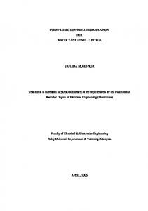
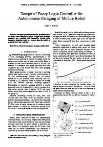
Equations 1 and 2 form the basis for controller design. They are simplified from more comprehensive building thermal models, for example by assuming a net sensible heat load and greenhouse solar heating efficiency. However, they are adequate to demonstrate the FLC design methodology and to make comparisons to the CSC. Block diagram equivalent forms for equations 1 and 2 are given in figures 1a and 1b (Mathworks, 1999). These block diagrams consist of multiple input-single output (MISO) systems, with input-output ports labeled numerically. All ports are placed on the right-most part of each model for identification. The greenhouse dynamic . building model contains four inputs (ventilation rate, V; supplemental heat, qheater and aSAf; outside temperature, Tout; solar irradiance, S). The broiler house model contains similar inputs (except irradiance) and output, but net sensible heat load is specified within the block. Each building model is stored in a masked block, as are the outside temperature and radiation blocks. Values for all model parameters (table 1) are specified at the block parameter screen. These building models can be used as components to various higher level models for the coupled controller/building system. DYNAMIC ENVIRONMENT CONTROL MODEL A dynamic environment control simulation system is illustrated in figure 2 for both greenhouse and broiler house. The system consists of three main blocks (input, controller, and building thermal model). Two types of controller (CSC and FLC, see fig. 3) are embedded in this dynamic simulation platform. The input to the CSC is temperature difference. The FLC takes up to two inputs (temperature difference and energy use). The system operation can be understood by tracing it, starting at the left-most summation block where the building interior temperature is subtracted from the building setpoint temperature. For example in the CSC case, the resultant temperature difference is passed into the controller block (fig. 3a). The CSC consists of a quantizer to obtain the appropriate stage of heating or ventilation, where negative values refer to stages of heating (current temperature is too low) and positive values refer to ventilation stages (current temperature is too high). The quantizer block serves to discretize the control error into discrete levels, q, that are specified by the user: output = q (round (input/q). For a 1°C quantization level, the quantized signal consists of one of a series of integers [. . . –3, -2, –1, 0, 1, 2, 3, . . .]. Thus for example, if temperature difference is +2.4°C then quantized output is 2. This provides a q/2 hysteresis about each stage transition. This approach can use any value for q, but is limited to constant stage differentials, which are adequate to demonstrate the process. The quantized output is interpreted as a ventilation or heat stage. To transform the heating or ventilation stage into a value for supplemental heat and/or ventilation rate, the VOL. 43(6): 1885-1894

(a)

(b) Figure 1–Dynamic models (a) greenhouse, equation 1, (b) broiler house, equation 2. Table 1. Building and simulation parameters used in study Building Parameters

Symbol Value Greenhouse

Heat losses Dimensions Volume Ventilation stages (1,2) Heating stage (1)

UA V. V q heater

425 W °C–1 5.2 × 14.6 × 3.1 m 240 m3 [2.05, 3.45] m3 s–1 30.5 kW

Broiler House Heat losses Dimensions Volume Heat production (30,000 birds) Ventilation stages (0-6) Heating stages Minimum ventilation Air density Specific heat Stages: Stage differential:

UA V q.internal V qheater ρ Cp CSC FLC CSC FLC

1868 W °C–1 12 × 156 × 2.4 m 4500 m3 [0, 150, 300] kW [4.7, 9.4, 18.8, 37.6, 56.4, 75.2, 75.2] m3 s–1 [300, 200, 0] kW Stage ‘0’ of ventilation 1.2 kg m–3 1006 J kg–1 [–1 0 1 2 3 4 5 6] [ -2 –1 0 1 2 3 4 5 6] 1°C Variable, according to fuzzy inference

quantized signal is passed to two switch blocks in series with two lookup tables (fig. 3). The top switch block/lookup table combination serves to select the appropriate ventilation rate, 1887

se 1844 ms

7/10/01

9:56 AM

Page 1888

Figure 2–Controller and equipment dynamic simulation system.

and the bottom switch block/lookup table combination selects the magnitude of supplemental heat. Each switch block passes through the value of the top input if the centerline input is greater than or equal to a specified value, otherwise the bottom line input is passed through. In this way the signed series of quantized values is split into negative and positive components for heating and ventilation, respectively. These quantized values then pass into table lookup blocks (fig. 3), which provide a numerical value for ventilation and heat stages. The supplemental heat and ventilation rate are passed to the masked “house” block. This masked block contains the components in figures 1a or 1b for greenhouse and broiler house, respectively. Outside temperature is generated as a sinusoidal input, and solar radiation as a Gaussian input. These inputs (ventilation rate, heating rate, outside temperature, and either solar load or net building sensible load) comprise the current state. The appropriate differential equation 1 or 2 is integrated to obtain inside temperature at the next time step. A Runge-Kutta integration algorithm with fixed time step (30 s) to represent the controller’s sampling rate was used. FUZZY LOGIC CONTROLLER DESIGN The fuzzy logic process was implemented with five operations: 1. Fuzzify numerical inputs based on measurement (e.g., temperature difference and/or energy use) using input membership functions. 2. Apply fuzzy operators to the antecedents of the rule base. 3. Perform implication, i.e., shape the consequent portion of the rules. 4. Aggregate each rule’s output into a common fuzzy set.

1888

(a)

(b) Figure 3–Controller simulation blocks: (a) stage controller, (b) fuzzy logic controller. Controller output is a discrete number (–2 to 6) representing stage of control. The switch blocks pass through the top input if the center input exceeds zero, else they pass through the bottom input. The switch blocks output are used in the table lookup blocks to assign ventilation rate or heating rate to the stage of control.

TRANSACTIONS OF THE ASAE

se 1844 ms

7/10/01

9:56 AM

Page 1889

Table 2. Rule base for the simple FLC (6 rules) Temperature Difference PBD PMD PSD ZD NSD NBD

Consequent Cooling-high Cooling-medium Cooling-low No-change Heat 1 Heat 2

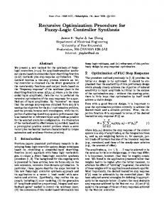
5. De-fuzzify the aggregate fuzzy set to obtain control output using a center of gravity output rounded to the nearest integer. The Fuzzy Logic Toolbox (Mathworks Inc., Natick, Mass.) was used to design the FLC. To demonstrate the FLC design, first consider a simple one-input and one-output FLC for a broiler house. The input, temperature difference, is identical to that provided to the CSC. Input membership functions for the temperature difference use six linguistic variables to apportion over the range of –6°C to +8°C (NBD, NSD, ZD, PSD, PMD, and PBD), following a method that is customary in the literature (e.g., Gates et al., 1997, 1998, 1999). For example, NBD refers to a Negative Big Difference between inside temperature and setpoint, i.e., it is much colder than desired in the building. The rule base for the simple FLC is given in table 2. Each possible linguistic value of input is assigned a consequential action; for example if input temperature difference is PBD then control action is “cooling-high”. A rule base maps linguistic inputs to outputs and the fuzzy process quantifies these actions. Inputs to the FLC are sent to a FLC block in the dynamic simulation (fig. 3b) which in turn maps these inputs to a desired output as explained previously. For example, if the FLC output were stage 6, then the ventilation rate would be 75.2 m3s–1 and the heating rate would be zero (see table 1). The connection between inputs and outputs, both of which are “crisp” values, is made via the linguistic transformation of inputs using input membership functions, implication and aggregation using the rule base, and de-fuzzification of the linguistic output to a numerical value representing stage of ventilation. Each process is described by means of example below. In a CSC, the stage differential can be used to some extent to dictate a trade-off between magnitude of temperature difference between building and set point, and amount of energy used. For the two different input membership functions depicted in figures 4a and b, a similar functionality can be obtained by specifying the amount of overlap between grades of membership. Figure 4a illustrates a fine degree of overlap, or mapping, between input control error and linguistic output variable; figure 4b is an example of a much coarser mapping. Both membership functions map control error in the range –6 to +8°C, so the degree of overlap dictates how finely the membership grades are split. An output membership function (fig. 4c) performs the process of implementing rules, and aggregating a response to provide a crisp output command. The output membership functions chosen in this example consist of two stages of heat (heat 2, heat 1) that may represent for example two different supplemental heating levels, with heat 2 being greater than heat 1. Working from cold to hot, VOL. 43(6): 1885-1894

(a)

(b)

(c) Figure 4–Membership functions for the simple FLC (a) input fine mapping, (b) input coarse mapping, and (c) output.

the next four membership grades are No change, Coolinglow, Cooling-medium, and Cooling-high. These each cover a range of possible heating/ventilating stages. Overlap of these functions is avoided because an integer output that represents “stage” is desired. The rule base listed in table 2 demonstrates how the linguistic variables, obtained from fuzzification, are used to aggregate a response using expert intuition. When coupled with an output membership function and appropriate defuzzification, a crisp control response is produced. In this case the control response will be a stage of heating or ventilating from the set [–2, –1, 0, 1, . . . , 6]. Figure 5 illustrates the entire FIS process for the two different input membership functions in figure 4 (fine versus coarse mapping). Each row of plots corresponds to a rule in table 2, and the two columns correspond to the input (left) and output (right) membership functions. The vertical line on the input membership functions demonstrates the input crisp value and its effect on each input membership grade that it intercepts (only PBD in this case). The value of each grade is projected onto the output membership function (right-hand column of graph) by parsing the 1889

se 1844 ms

7/10/01

9:56 AM

Page 1890

Table 3. Partial rule base for the two-input FLC (21 rules total) Temperature Difference PBD PMD PSD PZD NZD NSD NBD

(a)

(b) Figure 5–The FIS process for (a) fine input membership mapping, and (b) coarse mapping. For a given temperature difference (3°C or 5.9°C) as input, each row of plots in left pane corresponds to a rule (table 2). Rule implication and fuzzy product operator is used to project onto the output membership function (right hand pane), and aggregate them with an Integer Center of Gravity function to obtain the crisp output (lower right-hand pane, Stage = 6).

corresponding rule and using the appropriate implication operator (product in this example). This has the effect of creating a peaked response in the output membership functions; had the conventional max operator been used the output membership function would be clipped rather than peaked. This was done to force centered outputs so that during aggregation an integer output could be obtained. Finally, each active output membership grade is aggregated (lower right-hand plot), the center of gravity determined, and the nearest integer value to this COG is used. This method was implemented as a special function in the Matlab Fuzzy Logic Toolbox, and we named it the Integer Center of Gravity (ICOG). It is conventional to COG except an integer output is forced. Other methods are certainly possible to accomplish similar results, including the use of a Sugeno-type FIS (Mathworks, 1998). Note how both input membership functions yield the same crisp output, i.e., stage 6 ventilation. However, the approximate temperature difference for the finely mapped 1890

Energy Use Input Low

OK

High

Cooling-high Cooling-low No change No change No change No change Heat 2

Cooling-high Cooling-medium Cooling-low No change No change Heat 1 Heat 2

Cooling-high Cooling-high Cooling-medium Cooling-low Heat 1 Heat 2 Heat 2

input membership function is 3°C; whereas, it is 6°C for the more coarsely mapped membership function. This illustrates the importance of tuning both input and output membership functions to achieve desired results. A second input, labeled Energy Use (ranging from zero to one), was added to form the two-input FLC system. It provides the relative importance that a user attaches to energy consumption. A low value near zero indicates that energy use should be low; a value near unity suggests that minimal temperature difference is desired. Note that the Energy Use input can also be thought of as a user-specified “control precision” input (range: zero to one) to indicate how closely the system should try to track the set point. The input membership function for temperature difference uses three linguistic variables (Low, Ok, High). The input membership function for the energy use input consists of three linguistic variables by splitting the deadband Zero Difference (ZD) term for the one-input FLC into a positive, PZD, and a negative, NZD, term. A more comprehensive rule base (table 3) is required, consisting of 21 rules (3 Energy Use × 7 Temperature Difference).

SIMULATIONS The behavior of the CSC and FLC was examined using the dynamic greenhouse and broiler house simulations. Building physical and thermal parameters are given in table 1. The building parameters used for the greenhouse simulation are typical of a “small greenhouse” or single zone in a building complex, with single stage of heat and two stages of ventilation. The building thermal parameters selected for the broiler house are taken from Gates et al. (1993) and represent a facility which experiences a tremendous range in thermal loads on the interior environment as birds mature and as outside conditions vary. The HVAC equipment is generally selected for extreme conditions. Heaters are sized for design winter temperature with no bird heat, and ventilation for a design summer condition with maximum sized birds (Colliver et al., 1999, 2000). Forcing functions and interior temperature set points for the simulations are illustrated in figure 6. Greenhouse simulations were performed using diurnal variation in solar radiation (0 to 700 Wm–2) and outside temperature (8 to 22°C), with two set point temperature step changes (4°C each) at 25,200 s and 72,000 s. This test challenges both heating and cooling modes and assesses controller recovery from set point disturbance. Comparison between CSC and FLC included graphs of equipment switching and interior temperature.

TRANSACTIONS OF THE ASAE

se 1844 ms

7/10/01

9:56 AM

Page 1891

Figure 7–Simulated temperature response and controls for the FLC compared with the CSC.

Figure 6–Forcing functions and set points for greenhouse and broiler house simulations.

Broiler house simulations were performed using two combinations of set point and outside temperature patterns. In the first combination, outside temperature was constant (10°C), and building setpoint was varied in two steps (start at 20°C for 60 min, step-up to 25°C for 60 min, then stepdown to 20°C for 60 min). In the second combination, outside temperature increased in 5°C steps from –5 to 20°C, 60 min at each step, with constant building setpoint temperature (20°C). The first test primarily challenges steady-state performance of the system. The second test provides information of the dynamic response and recovery to steady state. Two bird-heat loads (0 and 300 kW) were selected to mimic small and mature broilers. Results were evaluated by comparing root mean square (RMS) of temperature difference between simulated building temperature and specified set point.

controller responses to the same disturbance (fig. 8). With Energy Use set to 0.75, interior temperature closely tracked set points; whereas, with Energy Use set to 0.25, considerable excursion from set points was realized. The control (equipment activation) plots show that FLC (0.75) used more heating and ventilation energy. During the nighttime heating mode, FLC (0.25) caused more frequent switching from heating to the minimum ventilation stage (less energy cost). Similarly, during the daytime ventilation mode, FLC (0.25) caused the equipment to stay at the minimum ventilation stage, while FLC (0.75) entered the maximum ventilation stage one-third of the time. In addition, FLC (0.75) caused earlier activation, and later deactivation, from the minimum ventilation stage. Provision of an Energy Use input allowed the two-input FLC controller to span the behavior of CSCs at a user’s request. BROILER HOUSE Simulation results of broiler house control system responses (CSC vs FLC) to constant outside temperature,

RESULTS GREENHOUSE Figure 7 shows simulated greenhouse control system (CSC vs FLC) responses to forcing functions (fig. 6). The one-input (temperature difference only) FLC exhibits dynamic response to the setpoint changes similar to that of the CSC. The nighttime temperature deviation was less than 0.1°C for both CSC and FLC. Neither system could maintain daytime temperature control when outside temperature rose to near the desired interior temperature. The CSC system resulted in temperatures slightly below those of the FLC system, except for a short time before and after the maximum, when the difference was reversed. Performance of the two-input (i.e., temperature difference, and Energy Use) FLC for the greenhouse illustrates how the second input can create a spectrum of VOL. 43(6): 1885-1894

Figure 8–Simulated temperature response and controls for the twoinput FLC. 1891

se 1844 ms

7/10/01

9:56 AM

Page 1892

Table 4. Controller root mean square error performance index (°C) as affected by step change in set point temperature (20/25/20°C) with outside temperature at 10°C. Each test was run for the indicated period of time. Conventional Stage Controller (CSC)

Fuzzy Logic Controller (FLC)

---------------------------Net Sensible Heat Production--------------------------0 300 0 300 kW kW kW kW Set Point Time (°C) (min) 20 25 20

Energy Use/Control Precision Setting Selection 0

0-30 0.7 30-60 1.1 60-90 0.8

Mean

2.1 1.3 2.4

2.6 3.1 2.5

0.25

0.5

0.75

1.0

0

0.25

0.5

0.75

1.0

1.8 2.3 1.8

0.2 1.0 0.5

0.3 1.0 0.6

0.5 1.1 0.6

3.6 3.2 3.8

2.3 2.0 2.6

2.1 1.4 2.3

1.5 0.6 1.6

0.4 0.6 0.7

0.88 1.96 2.74 1.95 0.66 0.69 0.76 3.50 2.29 1.96

1.33 0.56

Table 5. Controller root mean square error performance index (°C) as affected by series of outside temperature values. Each test was run for the indicated period of time Conventional Stage Controller (CSC)

OutSide Temp Time (°C) (min) –5 0 5 10 15 20

Fuzzy Logic Controller (FLC)

---------------------------Net Sensible Heat Production--------------------------0 300 0 300 kW kW kW kW Energy Use/Control Precision Setting Selection 0 0.6 0.8 1.2 2.1 2.7 4.3

3.0 3.0 2.8 2.7 2.7 1.2

0.25

0.5

0.75

1.0

0

0.25

0.5

0.75

1.0

2.2 2.2 1.9 1.8 1.8 1.9

0.2 0.2 0.2 0.2 0.2 0.2

0.5 0.4 0.4 0.3 0.2 0.1

0.8 0.8 0.5 0.5 0.3 0.1

2.5 2.7 3.3 3.7 4.2 5.2

0.4 1.9 2.1 2.3 3.6 4.6

0.6 1.2 1.4 2.1 2.6 4.3

0.5 0.2 0.5 1.5 1.9 3.9

0.9 0.9 0.7 0.4 1.3 3.2

0-30 30-60 60-90 90-120 120-150 150-180

1.2 0.9 0.8 0.7 0.7 0.2

Mean

0.75 1.95 2.57 1.97 0.20 0.32 0.50 3.60 2.48 2.03

1.42 1.23

step changes in set point and two different bird heat loads (fig. 6) are provided in table 4. The RMS error performance index for the CSC coincided approximately with that for the two-input FLC with Energy Use set to 0.5. A strong influence of internal heat production is apparent: the performance index for CSC more than doubled (0.9 to 2.0°C), while that for the FLC increased at low energy use settings (increase of 0.8 to 0.3°C) but decreased by 0.2°C at the highest energy use setting. Performance index was greater at the higher set point for CSC and FLC at low energy use settings, but lower for FLC at higher energy use settings. This demonstrates the flexibility of the FLC to reduce temperature difference by using more energy, or to allow the temperature difference to float higher than the CSC and reduce energy use. A series of step changes in outside temperature, with constant interior set point, demonstrates how internal loads can impact steady-state interior temperature, hence performance index (table 5). A step change in outside temperature is not physically realistic, but it serves to test the controller’s disturbance rejection ability, and the 30 min period between step changes provided ample time for steady state to be achieved. With no internal heat load, the CSC and the FLC (low energy use settings) both realized greater performance degradation at warmer outside conditions. However, for energy use settings greater than about 0.5, the FLC improved the performance index at warmer outside conditions. Mean performance index values were 0.75°C for the CSC versus 2.6 to 0.5°C for the FLC. The principal effect of interior heat load on the broiler simulations (from 0 to 300 kW) was a nearly 300% increase in the performance index for CSC, and 50% to 1892

over 400% increase for the FLC. CSC performance was again on par with the FLC with a 0.5 energy use setting. The performance index varied from 3.6°C to 1.2°C as energy use setting was varied from 0 to 1; by comparison the respective CSC value was 1.95°C.

DISCUSSION None of the performance index values from the broiler simulations are considered excessive in terms absolute error (maximum under 4°C), nor are they spectacular in comparison to expected errors for a control system that is not based on discrete outputs, e.g., a PID system. However, these small differences of a few degrees can have a tremendous impact on seasonal energy use. For example, for a rural electric cooperative that services 500 broiler houses, with each house requiring 8 kW for ventilation energy, a one-stage reduction from the highest stage of ventilation represents about 2 kW/house. This represents 1000 kW peak demand reduction. Most of this reduction occurs during swing periods when outside temperature is either rising or falling. This latter case corresponds to peak residential uses for many utility systems. In contrast to energy savings, building operators challenged to obtain more precise adherence to building temperature “blueprint” schedules may select a higher energy use setting during critical periods and then reduce the setting during less critical periods. The FLC methodology presented is straightforward to implement in any existing CSC which utilizes a microprocessor with floating point capability. The proposed design concept incorporates the discrete nature of existing staged ventilation equipment. Centralized computer-controlled facilities can also adopt the FLC strategy on the central computer, and download adjustments to CSC set point. This would provide robust, predictable CSC behavior in event of a fault (Sigrimis, 1999; Sigrimis et al., 2000b). Adoption of the FLC technique presented here has several key advantages. A principal advantage is that the building operator has a preferential input to balance energy use and control precision. Conventional staged controllers provide this to a limited extent, by using variable differential temperatures between stages. But as they act as discrete proportional controllers, a CSC cannot approach a zero steady-state control error. In contrast, the FLC with Energy Use input gives integrator-like behavior, and can further reduce steady-state control error. The FLC retains the robustness and flexibility of the CSC, with enhanced control features including recovery from step and diurnal disturbances. The ability of the FLC to work equally well in vastly different building scales in particular makes this an attractive technological feature to commercial environment control systems. The simulation methodology used in this work can be useful for design purposes and for teaching dynamic systems and their design.

CONCLUSIONS Simple non-steady-state heat balance equations were used in conjunction with greenhouse and broiler house dynamic models to simulate conventional and fuzzy-based, staged control system performance. Comparisons between TRANSACTIONS OF THE ASAE

se 1844 ms

7/10/01

9:56 AM

Page 1893

the new fuzzy stage controllers and conventional staged control were made. The proposed fuzzy logic control (FLC) technique has the following advantages over conventional stage control (CSC) systems: 1. The FLC is scalable over a range of building sizes. 2. The FLC can provide a trade-off between departure from set point and energy use. A user-defined input of Energy Use is intuitive and can be effectively implemented. 3. The FLC may be implemented in a particular building with less complexity than the CSC, as there is no specification for stage differentials, hysteresis, etc. 4. The FLC may be implemented on any existing microprocessor-based CSC systems that have floating point capability. ACKNOWLEDGMENTS. This research was supported in part by USDA Regional Project S-261, “Interior Environment and Energy Use in Poultry and Livestock Facilities”, and S-291 “Systems for Controlling Air Pollutant Emissions and Indoor Environments of Poultry, Swine, and Dairy Facilities”.

REFERENCES ACME. 1993. The Greenhouse Climate Control Handbook, Engineering Principles and Design Procedures. Muskogee, Okla.: ACME Engineering & Manufacturing Corp., Horticultural Division Albright, L. D. 1990. Environment Control for Animals and Plants. St. Joseph Mich.: ASAE. AMCA. 1995. Fan Application Manual. Air Movement and Control Association. Arlington Heights, Ill. Aminzadeh, F., and M. Jamshidi. 1994. Soft Computing. Englewood Cliffs, N.J.: PTR Prentice Hall. Berckmans, D., and V. Goedseels. 1986. Development of new control techniques for ventilation and heating of livestock buildings. J. Agric. Eng. Res. 33: 1-12. Chao, K., R. S. Gates, and H.-C. Chi. 1995. Diagnostic hardware/software system for environment controllers. Transactions of the ASAE 38(3): 939-947. Chao, K. 1996. Economic optimization of single stem rose production. Unpub. Ph.D. diss. Lexington, Ky.: Biosystems and Agricultural Eng. Dept., University of Kentucky. Chao, K., and R. S. Gates. 1996. Design of switching control systems for ventilated greenhouses. Transactions of the ASAE 39(4): 1513-1523. Chao, K., R. S. Gates, and R. G. Anderson. 1998a. Knowledgebased control systems for single stem rose production: Part I. systems analysis and design. Transactions of the ASAE 41(4): 1153-1161. ______. 1998b. Knowledge-based control systems for single stem rose production: Part II. implementation and field evaluation. Transactions of the ASAE 41(4): 1163-1172. Chen, G. 1996. Conventional and fuzzy PID controllers: An overview. Int. J. Intel. Control & Sys. 1(2): 235-246. Cole, G. W. 1980. The application of control systems theory to the analysis of ventilated animal housing environments. Transactions of the ASAE 23(2): 431-436. Colliver, D. G., R. S. Gates, T. F. Burks, and H. Zhang. 2000. Development of the design climatic data for the 1997 ASHRAE Handbook - Fundamentals. ASHRAE Trans. 106(1): 3-14. Colliver, D. G., T. F. Burks, and R. S. Gates. 1999. ASHRAE Design Weather Data Viewer. (CD-ROM Ver. WDVIEW2.1). ISBN 1883413-75-3. American Society of Heating, Refrigerating and Air-Conditioning Engineers, Inc., Atlanta, Ga. VOL. 43(6): 1885-1894

Colliver, D. G., H. Zhang, and R. S. Gates. 1998a. ASHRAE Design Weather Sequence Viewer (CD-ROM Ver. 2.1). ISBN 1-883413-64-8. American Society of Heating, Refrigerating and Air-Conditioning Engineers, Inc., Atlanta, Ga. Colliver, D. G., R. S. Gates, H. Zhang, and K. T. Priddy. 1998b. Development of the sequences of extreme temperature and humidity for design conditions (828-RP). ASHRAE Trans. 104(1): 133-144. Ford, S. E., L. L. Christianson, G. L. Riskowski, and T. L. Funk. 1993. Agricultural ventilation fans, Performance and efficiencies. Bioenvironmental and Structural Systems Laboratory (BESS), Agricultural Engineering Dept., University of Illinois at UrbanaChampaign, Ill. Gates, R. S., and M. B. Timmons. 1986. Real-time economic optimization of broiler production. ASAE Paper No. 86-4552. St Joseph Mich.: ASAE. Gates, R. S., and M. B. Timmons. 1987. Microprocessor controlled broiler environment for optimal production. In Proc. 2nd Technical Session of the CIGR on Latest Developments in Livestock Housing, 220-235, University of Illinois, UrbanChampaign, Ill., 22-26 June 1987. St Joseph, Mich.: ASAE. Gates, R. S., and M. B. Timmons. 1989. Economic optimization of tom turkey production. Poultry Sci. 68(4): 470-475. Gates, R. S., D. G. Overhults, B. L. Walcott, and S. A. Shearer. 1991. Constant velocity air inlet controller. Computers & Electronics in Agric. 6: 175-190. Gates, R. S., L. W. Turner, and D. G. Overhults. 1992a. Transient overvoltage testing of environmental controllers. Transactions of the ASAE 35(2): 727-733. _____. 1992b. A survey of environmental controllers. Transactions of the ASAE 35(3): 993-998. Gates, R. S., D. G. Overhults, and L. W. Turner. 1992c. Mechanical backup systems for electronic environmental controllers. Applied Engineering in Agriculture 8(4): 491-497. Gates, R. S., D. G. Overhults, R. W. Bottcher, and S. H. Zhang. 1992d. Field calibration of a transient model for broiler misting. Transactions of the ASAE 35(5): 1623-1631. Gates, R. S., H. Minagawa, M. B. Timmons, and H. Chi. 1994. Economic optimization of Japanese swine production. ASAE Paper No. 94-4085. St Joseph, Mich.: ASAE. Gates, R. S., M. B. Timmons, D. G. Overhults, and R. W. Bottcher. 1997. Fuzzy reasoning for environmental control during periods of heat stress. In Livestock Environment V, Vol I, eds. R. W. Bottcher, and S. J. Hoff, 553-562. St. Joseph, Mich.: ASAE. Gates, R. S., K. Chao, and N. Sigrimis. 1998. Design parameters for fuzzy-based control of agricultural ventilation systems. In Control Applications and Ergonomics in Agriculture, First Workshop on Intelligent Control for Agricultural Application, 137-142. Oxford, U.K.: Int. Federation of Automatic Control, IFAC Pub., Elsevier Science Ltd. Gates, R. S., K. Chao, and N. S. Sigrimis. 1999. Fuzzy control simulation of plant and animal environments. ASAE Paper No 99-3136. St. Joseph, Mich.: ASAE. Harriman, L. G., D. G. Colliver, and K. Q. Hart. 1999. New weather data for energy calculations. ASHRAE J. 41(3): 31-38. Malki, H. A., D. Misir, D. Feigenspan, and G. Chen. 1997. Fuzzy PID controller of a flexible-joint robot arm with uncertainties from time-varying loads. IEEE Trans. Control Systems Technol. 5(3): 371-378. Marsh, L. S., and L. D. Albright. 1991. Economically optimum day temperatures for greenhouse hydroponic lettuce production. Parts I & II. Transactions of the ASAE 34(2): 550-562. Martin-Clouaire, R., and K. Kovats. 1993. Satisfaction of soft constraints applied to the greenhouse to the determination of greenhouse climate setpoints, 211-220. In Proc. AIFA Conf., Artificial Intelligence for Agriculture and Food, Equipment and Process Control, 27-29 Oct., Nimes, France. London, England: Elsevier, Ltd.

1893

se 1844 ms

7/10/01

9:56 AM

Page 1894

Mathworks Inc. 1998. 3rd Printing. Fuzzy Logic Toolbox User’s Guide, Ver. 2. Natick Mass.: The Mathworks Inc. _____. 1999. Using Simulink, Ver. 3. Natick Mass.: The Mathworks Inc. Sigrimis, N., and R. King. 2000. Advances in greenhouse environment control. Computers & Electronics in Agric. 26(3): 321-342. Sigrimis, N. A., K. G. Arvanitis, and R. S. Gates. 2000a. A learning technique for a general purpose optimizer. Computers & Electronics in Agric. 26(2): 83-103. Sigrimis N., K. G. Arvanitis, G. D. Pasgianos, and N. Rerras. 2000b. Synergism of high and low level systems for the efficient management of greenhouses. Computers & Electronics in Agric. 29(12): 21-39. Sigrimis, N. 1999. Computer integrated management and intelligent control of greenhouses. Fourteenth IFAC World Congress, Beijing, PRC, 4-11 July, Pre-congress Workshop on Intelligent Control Systems in Agriculture (Tutorial Workshop #8), Plenary Volume. Oxford, U.K.: Elsevier Science, Ltd. Sigrimis, N., A. Anastasiou, and N. Rerras. 1999. Energy saving in greenhouses using temperature integration: A simulation survey. Computers & Electronics in Agric. 26(3): 321-342. Sigrimis, N., and N. Rerras. 1996. A linear model for greenhouse control. Transactions of the ASAE 39(1): 253-261. Timmons, M. B., and R. S. Gates. 1986. Economic optimization of broiler production. Transactions of the ASAE 29(5): 13731378,1384. _____. Gates. 1987. Relative humidity as a ventilation control parameter in broiler housing. Transactions of the ASAE 30(4): 1111-1115.

1894

Timmons, M. B., R. S. Gates, R. W. Bottcher, T. A. Carter, J. Brake, and M. J. Wineland. 1995. Simulation analysis of a new temperature control method for poultry housing. J. Agric. Eng. Res. 62: 237-245. Ting, K. C., and G. A. Giacomelli. 1991. Systems integration of automation, culture and environment within CEA, 513-526. In Proc. 1991 Symp. on Automated Agriculture for the 21st Century. St. Joseph, Mich.: ASAE. USDA. 1999. Interior environment and energy use in poultry and livestock facilities. Regional Project S-261. For final report and home page: http://www.bae.uky.edu/~gates/Research/ s291/s291.htm. Zhang, Y., and E. M. Barber. 1993. Effects of control strategy, size of heating/ventilation equipment and controller time constant on thermal responses and supplemental heat use for a livestock building. In Livestock Environment IV, 347-355, eds. E. Collins, and C. Boon. St. Joseph, Mich.: ASAE. Zhang, G., S. Morsing, and J. S. Ström. 1993a. An airflow pattern control algorithm for livestock buildings. In Livestock Environment IV, 779-787, eds. E. Collins, and C. Boon. St. Joseph Mich.: ASAE. Zhang, Y., E. M. Barber, and H. C. Wood. 1993b. Analysis of stability of livestock building HVAC control systems. Trans. Am. Soc. Heat. Refrig. Air-Cond. Eng. 99(2): 237-244.

TRANSACTIONS OF THE ASAE