Digital temperature control and measurement system

Digital temperature control and measurement system R. B. Strem, B. K. Das, and S. C. Greer Citation: Review of Scientific Instruments 52, 1705 (1981); doi: 10.1063/1.1136517 View online: http://dx.doi.org/10.1063/1.1136517 View Table of Contents: http://scitation.aip.org/content/aip/journal/rsi/52/11?ver=pdfcov Published by the AIP Publishing Articles you may be interested in Sonic digitizer coil measurement system J. Acoust. Soc. Am. 90, 2883 (1991); 10.1121/1.401798 A digital temperature control system Rev. Sci. Instrum. 62, 1311 (1991); 10.1063/1.1142491 Digital controller for a magnetic suspension system Rev. Sci. Instrum. 57, 1616 (1986); 10.1063/1.1138540 Magnetic suspension systems with digital controllers Rev. Sci. Instrum. 57, 1611 (1986); 10.1063/1.1138539 Measuring‐while‐drilling method and system having a digital motor control J. Acoust. Soc. Am. 65, 559 (1979); 10.1121/1.382379

This article is copyrighted as indicated in the article. Reuse of AIP content is subject to the terms at: http://scitationnew.aip.org/termsconditions. Downloaded to IP: 129.2.19.102 On: Mon, 19 Oct 2015 16:00:50

Digital temperature control and measurement system R. B. Strem, B. K. Das, and S. C. Greer Department of Chemistry. University of Maryland. College Park. Maryland 20742 (Received 3 June 1981; accepted for publication 2 August 1981)

We describe an automated digital temperature control and measurement system with a temperature resolution of about 1 mK and operating in the temperature range - 40· to + 70 ·C. PACS numbers: 07.20.Dt

I. INTRODUCTION

In modern measurements ofthermodynamic properties, the temperature must be precisely controlled (millikelvin or better), often for long periods of time. The standard practice has been to use analog controllers to control liquid baths, vacuum thermostats, and layered thermostats. I - 6 Digital temperature control systems have been reported for a O.I-K controller by PomernackF and for the sample temperature control in a calorimeter by Martin et al. 8 •9 The recent appearance of inexpensive microcomputers and the proliferation of instruments bearing the IEEE-488 IO computer interface bus now make a digital temperature control and measurement system a simple and attractive alternative to analog controllers for control of a millidegree or better. In addition to controlling and measuring the temperature, a digital controller offers a particularly convenient mechanism for stepping the temperature at required time and temperature intervals. Moreover, the same microcomputer can collect data from experimental transducers. We have built a digital temperature measurement and control and data acquisition system with proportional and integral temperature control. ll - 13 With a vacuum thermostat and auxiliary cooler, we can control and measure temperature between -40° - + 70°C with a precision of about 1 mK. II. HARDWARE A. Thermostat

The thermostat we are using with the digital controller is a multistage vacuum thermostat of conventional design. The thermostat consists of three stages: an outer vacuum can, an inner can or radiation shield, and the experimental stage. The two cans are evacuated independently through vacuum lines. The vacuum lines and the connections between stages are made of thin-walled stainless-steel tubing. Vacuum connections are made with elastomer o-rings .14 The outer can is made of aluminum, which provides good thermal conductivity with minimal weight. A commercial cooler-circulator l5 controls the temperature of a circulating fluid to 0.02 K between 40° - - 50°C and pumps that fluid through aluminum tubing wrapped around the outer can. The radiation shield is made of copper; a heater wire of 338 0 is wrapped in grooves around the can. The experimental 1705

Rev. Sci. Instrum. 52(11), Nov. 1981

stage is also made of copper. Electrical leads enter the thermostat from a vacuum feedthrough and are thermally grounded. A vacuum of about 10-3 mm Hg is maintained in the thermostat. We estimate the total heat transfer from the interior of the thermostat to the cooler by radiation and conduction to be about 0.2 W when the vacuum can is at 234 K and the radiation shield and experimental stage are at 233 K. The total thermostat heat capacity is about 8 x 103 J/K. B. Thermometry

The control thermometer (T2 in Fig. 1) is a 4-kO thermistor mounted on the radiation shield. The measurement thermometers ate a 100-0 platinum resistance thermometer (Tl) and a 4-kO thermistor (T3), both mounted on the experimental stage. Tl is shown in Fig. 1; T3 is not shown, but its circuit is identical to that of T2. Each thermometer is in series with a standard resistor [Rl (1250 0), R2 (50 kO), R3 (50 kO)), and a mercury battery. If RT is the resistance of the thermometer, V T the voltage drop across the thermometer, and V s the voltage drop across the standard resistor, then RT = (VTIVs)R s. T2 and T3 are bead thermistors with expected stabilities of 0.05% (or 13 mK) per year. 16 The temperature coefficient of Tl is about 0.4% per degree and that for T2 and T3 is about 4% per degree. The standard resistors have a temperature coefficient of 1 ppm/K and a stability of 5 pprniyr. 17 V T and V s are measured by a 6 ~-digit voltmeter l8 in a four-wire configuration to eliminate lead resistances. The standard resistors were so chosen as to keep currents low enough that self-heating is not important. The standard resistors and batteries were wrapped in thermal insulation to improve their stability. The long-time stability of the controller is determined by the stabilities of the control thermometer (13 mK/yr) and its standard resistor (about 0.2 mK/yr). The stability of the control set point to changes in room temperature is, from the temperature dependence of the standard resistor, about 0.03 mK for a change of 1 K in room temperature. Since the ratio V TIVs is used, drifts in the voltmeter cancel out. The platinum thermometer was calibrated by the National Bureau of Standards to 1 mK on the International Practical Temperature Scale of 1968. The thermistors

0034-6748/81/111705-04$00.60

© 1981 American Institute of Physics

1705


were calibrated with respect to the platinum thermometer. Polynomial least squares fits were obtained of the temperature as functions of RT for the platinum thermometer, and of In RT for the thermistors. 19,20 With a voltage resolution of 1 p. V, we can resolve 3 mK on the platinum thermometer and 0.3 mK on the thermistors. For a measurement thermometer used in a dc circuit such as we have, thermal emfs can be important (a few mK). Thermal emfs average out if the battery voltage is reversed (by the computer via relays or by replacing the battery with a D/A converter with reversible polarity) and V T and V~ averaged over the two current directions.

I.3!5V RADIATION SHIELD

T2 EXPERIMENTAL STAGE

SCANNER RI

C. Feedback loop

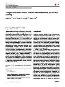
Figure 1 shows a block diagram of the hardware of the feedback loop. A scanner21 (multiplexer) allows us to read all the thermometer voltages with one voltmeter. 18 Both the scanner and the voltmeter are under the control of the microcomputer. 22 The computer calculates the radiation shield and experimental stage temperatures from the voltages, using the calibration equations. The temperature of the radiation shield is compared to the desired temperature and the difference used to adjust the heater voltage by means of a digital-to-analog (0/ A) converter 2:J which drives a programmable power supply. 24 The scanner, voltmeter, and 0/ A converter all connect to the computer via the IEEE-488 interface bus. 25 III. SOFTWARE A. General

The computer brings the radiation shield temperature to a desired value and controls it at that temperature until the experimental stage reaches that same temperature (within a given discrepancy) and remains so for a given time. Then the computer collects the experimental data, which are voltages on the other channels of the scanner (not shown in Fig. 1). During the data collection, the temperature control is suspended and the voltage to the shield heater remains constant at the last value calculated for it. The experimental stage is so isolated from the shield that the temperature drift at the experimental stage does not exceed a millikelvin during the short time of the data collection (a few minutes). The data are recorded on a cassette recorder and on a printer. Then the computer increments the temperature and repeats the procedure. B. Feedback loop

The feedback control consists of integral and proportional controP1-13 of the radiation shield temperature. The experimental stage temperature follows the shield temperature, mainly by gas conduction. We use the following symbols: To = Temperature of outer vacuum can, T[) = Desired temperature of radiation shield and experimental stage, Ts = Actual temperature of radiation shield, TE = Actual temperature of experimental stage. The "proportional" control provides the power to 1706

Rev. Sci. Instrum., Vol. 52, No. 11, November 1981

FIG. I. Digital temperature control and measurement system. Tl and T2 are resistance thermometers. RI and R2 are standard resistors. The scanner and voltmeter read the voltage drops across TI, T2, Rl, and R2. The computer calculates the temperature from the voltage drops, compares the actual temperatures to desired temperatures, then applies an appropriate voltage to the heater via the digital-toanalog converter and the programmable power supply.

attain T[) when Ts is less than T/}. The power to the heater is proportional to the square of the heater voltage. If Vi'

is the needed heater voltage, then (1)

where Ap is a constant. If we consider this contribution to be primarily the heating of the shield itself, ignoring the slow heat loss to the experimental stage, then to a first approximation

(2) where R is the heater resistance, C p is the heat capacity of the shield, and t is the time allowed for the temperature change. The "proportional gain" Ap can be initially set via Eq. (2), then adjusted by trial and error to achieve maximum gain without oscillation. 11 - 1:1 The "integral" control provides for most of the power required to the radiation shield heater to maintain a given difference between To and T[). We designate this "steady-state voltage" by V~S and write (3)

where AI is a constant. AI can be determined empirically or estimated from the calculated heat loss. The functional relationship between Vss and (Ts - To) may be more complex than Eq. (3), but Eq. (3) is an adequate first approximation. The square of the total voltage applied to the heater is therefore (4) Digital temperature control

1706


YES

TIME SET:

SET FG=I

TI=O

FlAG SET: FG=O

SET

H=TI+C YES YES

V=O

FIG. 2. Flow diagram of computer program for temperature measurement and control. The symbols are: TD, desired radiation shield temperature; N, number of do-loops which increment TD by an amount t!..T; Tl, running real time on computer clock; FG, flag to indicate when temperature first comes to desired value; T s , actual radiation shield temperature; T E , actual experimental stage temperature; V, voltage applied to heater; A, allowed difference between Ts and TE during control; B, allowed difference between TD and Ts during control; C, equilibration time interval after control is achieved; H, real time at which data are to be collected.

SEND

V

TO D/A CONVERTER

WAIT SAMPLING INTERVAL

If (TD - Ts) > 0.2 K, then V p is set at a maximum programmable voltage. If TD is less than Ts, then the V is set to zero until TD is attained. Cooling is such a slow process in this thermostat that "proportional" cooling is not necessary. Figure 2 is a flow diagram of the control program, which is written in BASIC and easily fits within the 8 K memory of the microcomputer. The keyboard input allows the operator to enter the starting value of T D, the desired temperature increments IlT, the number of increments N, and the circulating cooler temperature To. If T D < T s , then no voltage is applied to the heater. If TD> Ts , then a voltage calculated from Eqs. (1)-(4) is applied to the heater. This determination ofTs relative to T D is done repeatedly, at a sampling interval of about 20 s. The control do-loop continues as long as lTD - Ts I > B, whereB is of the order of mill ikeIvin, or ITs - TE I > A, where A is of the order of 10-100 millikelvin. TI

is the running real time from the internal clock of the microcomputer. When lTD - Tsl < B and ITs - TEl < A, then control is maintained for a time C, after which the data are collected, TD is incremented, and a new control loop begins.

1707

Digital temperature control


IV. PERFORMANCE AND DISCUSSION

The time constant of our thermostat is quite long: When To is about 10K less than T D, an increase of I K requires about 5 h and a decrease of 1 K requires about 6 h. The cooling time constant is consistent with the estimated rate of heat loss of 0.2 W. The heating time constant is consistent with the thermostat heat capacity. The control system does not seem to be particularly sensitive to any of the control parameters-the constants Al and Ap or the sampling time. Typically Al = 15 V2/deg andAp = 40 V2/deg. The typical controlled 1707


heater voltage of 12 V for (Ts - To) = 10 K is consistent with the estimated heat loss. The temperature at the radiation shield is controlled with random deviations of less than 1 mK for indefinite periods of time. The control at the experimental stage depends upon the choice of A, but a running control near the level of the thermistor resolution (0.3 mK) can be achieved. In our system the interruption of shield control for data collection limits the experimental stage control to about 1 mK. An improved control at the experimental stage could be achieved by writing the control program in such a way that the temperature control continued during the data acquisition. More precise thermometry could then be achieved using a computer-automated ratio transformer bridge to measure the thermometer resistances. 8,9,26 ACKNOWLEDGMENTS

C. T. Van Degrift was an invaluable help to us in developing this system; the thermostat design and the computer hardware configuration closely follow his designs. We thank R. W. Gammon and D. T. Jacobs for helpful discussions. J. T. Siewick and W. T. Angel assisted in the thermostat construction. This work was supported by the Office of Naval Research.

1708


D. Sarid and D. S. Cannell, Rev. Sci. Instrum. 45, 1082 (1974). J. Dratler, Rev. Sci. Instrum. 45, 1435 (1974). 3 M. Grubic and V. Wurz, J. Phys. E. 11, 692 (1978). 4 P. H. Sydenhan and G. C. Collins, J. Phys. E. 8, 311 (1975). 5 T. M. Sporton, J. Phys. E. 5, 317 (1972). 6 B. J. Thijsse, J. Chern. Phys. 74, 4678 (1981). 7 C. L. Pomernacki, Rev. Sci. Instrum. 48, 1420 (1977). 8 D. L. Martin, L. L. T. Bradley, W. J. Cazemier,and R. L. Snowdon, Rev. Sci. Instrum. 44, 675 (1973). 9 D. L. Martin and R. L. Snowdon, Rev. Sci. Instrum. 41,1869 (1973). 10 D. Metcalfe, Electron. Eng. 49, 37 (1977). 11 E. M. Forgan, Cryogenics 14, 207 (1974) gives a brief and lucid discussion of feedback loops for temperature control. 12 James A. Cadzow and Hinrich R. Martens, Discrete-Time and Computer Control Systems (Prentice-Hall, Englewood Cliffs, NJ, 1970). 13 A. J. Allen and P. Atkinson, Radio and Electron. Eng. 42, 55 (1972). 14 Low temperature compound E540-80, Parker Seal Co., Lexington, Kentucky. 15 Circulator-cooler LT-50, Neslab Instruments Inc., Portsmouth, New Hampshire. 16 Type S-I, Thermometries, Inc., Edison, New Jersey. 17 Type HP202, Vishay Resistor Products, Malvern, Pennsylvania. 18 Model 3455A, Hewlett-Packard Co., Palo Alto, California. 19 M. Sapoff, Meas. Control 14, 110 (1980). 20 H. W. Trolander, D. A. Case, and R. W. Harruff, in Temperature-Its Measurement and Control in Science and Industry: Proceedings 4, Pt. 2, (Instrument Society of America, Pittsburgh, Pennsylvania, 1972), p. 997. 21 Model 3495A, Hewlett-Packard Co., Palo Alto, California. 22 Model PET 2001, Commodore Business Machines, Inc., Palo Alto, California. 23 Model SN488-031, Kepco, Inc., Flushing, New York. 24 Model 1P-2728, Heath Co., Benton Harbor, Michigan. 25 E. Fisher and C. W. Jenson, PET and the IEEE 488 Bus (GPIB) (Osborne/McGraw-Hili, New York, 1980). 26 P. Lucas and J. A. Donnelly, Rev. Sci. Instrum. 52, 582 (1981). 1

2

Digital temperature control

1708
