Dimensioning bandwidth for elastic traffic in high-speed data networks

IEEE/ACM TRANSACTIONS ON NETWORKING, VOL. 8, NO. 5, OCTOBER 2000

643

Dimensioning Bandwidth for Elastic Traffic in High-Speed Data Networks Arthur W. Berger, Senior Member, IEEE, and Yaakov Kogan, Senior Member, IEEE

Abstract—Simple and robust engineering rules for dimensioning bandwidth for elastic data traffic are derived for a single bottleneck link via normal approximations for a closed-queueing network (CQN) model in heavy traffic. Elastic data applications adapt to available bandwidth via a feedback control such as the transmission control protocol (TCP) or the available bit rate transfer capability in asynchronous transfer mode. The dimensioning rules satisfy a performance objective based on the mean or tail probability of the per-flow bandwidth. For the mean objective, we obtain a simple expression for the effective bandwidth of an elastic source. We provide a new derivation of the normal approximation in CQNs using more accurate asymptotic expansions and give an explicit estimate of the error in the normal approximation. A CQN model was chosen to obtain the desirable property that the results depend on the distribution of the file sizes only via the mean, and not the heavy-tail characteristics. We view the exogenous “load” in terms of the file sizes and consider the resulting flow of packets as dependent on the presence of other flows and the closed-loop controls. We compare the model with simulations, examine the accuracy of the asymptotic approximations, quantify the increase in bandwidth needed to satisfy the tail-probability performance objective as compared with the mean objective, and show regimes where statistical gain can and cannot be realized. Index Terms—Asymptotic approximation, asynchronous transfer mode, closed queueing networks, computer network performance, effective bandwidths, Internet, traffic engineering, transmission control protocol.

I. INTRODUCTION

T

HIS PAPER considers the problem of dimensioning bandwidth for elastic data applications in packet-switched communication networks, such as Internet protocol (IP) or asynchronous transfer mode (ATM) networks. Elastic data applications can adapt to time-varying available bandwidth via a feedback control such as the transmission control protocol (TCP) or the available bit rate (ABR) transfer capability in ATM. Typical elastic data applications are file transfers supporting e-mail or the World Wide Web. A contribution of this paper is to derive simple, closed-form dimensioning rules that satisfy a performance objective on per-flow or per-connection bandwidth. For the particular case of an objective on the mean per-flow bandwidth, we obtain a simple expression for the effective bandwidth of an elastic traffic source. Manuscript received March 10, 1998; revised April 20, 1999 and June 7, 2000; aprroved by IEEE/ACM TRANSACTIONS ON NETWORKING Editor J. Wong. A. W. Berger was with AT&T Labs, Middletown, NJ 07748 USA. He is now with Akamai Technologies, Cambridge, MA 02139 USA (e-mail: arthur@ akamai.com). Y. Kogan is with AT&T Labs, Middletown, NJ 07748 USA (e-mail yakov@ buckaroo.mt.att.com). Publisher Item Identifier S 1063-6692(00)09122-6.

We assume that the closed-loop controls for the elastic data applications are performing well. For the present work, the key attribute of a well-performing control is that it maintains some bytes in queue at the bottleneck link with minimal packet loss. In contrast, poorly performing controls oscillate between undercontrolling (leading to excessive packet or cell loss) and overcontrolling (where, for example, TCP needlessly enters a slow-start or a time-out state). Thus, poorly performing controls limit the user’s throughput below what would have been possible, given the available bandwidth. Our assumption of well-performing controls is consistent with ongoing research efforts to improve current controls. We focus on a single bottleneck target link and obtain a simple product-form closed-queueing network (CQN) model in heavy traffic. CQN models have been used extensively for the analysis and design of computer systems and networks, see, for example, [1] or [2], and our model is one of the simplest; though the entity modeled by a “job” is nonstandard, see Section II. Our CQN model consists of one infinite server (IS) and one processorsharing (PS) server and was motivated by Heyman, Lakshman, and Neidhardt, [3], who also use a CQN model where the focus is on analyzing the performance of the closed-loop control TCP in the context of Web traffic. An important practical feature of these CQN models is their insensitivity: the distribution of the underlying random variables influences the performance only via the mean of the distribution. Thus, given the assumptions of the model, our engineering rules pertain in the topical case when the distribution of file sizes is heavy-tailed [4], though with finite mean, and thus the superposition of file transfers is long-range dependent [5]. The assumption of processor sharing in the CQN model is needed for the theoretical results, and corresponds to an assumption that the output ports of the network nodes use some type of fair queueing across the class of elastic data flows/connections; for a recent review of implementation of various fair queueing algorithms, see Varma and Stiliadis [6]. However, the model predictions do not seem particularly sensitive to this assumption, as illustrated in Section VI-A by a comparison with simulations that used a first-in-first-out (FIFO) discipline. Since forecasted demand has significant uncertainty, we believe that simple ballpark dimensioning rules are appropriate. In order to attain such closed-form rules, we use a normal approximation, which pertains in the regime of interest: heavy traffic with many flows and with high-speed links. A second contribution of the paper is new derivations of the normal approximation that in particular provide an estimate on the error of this approximation. The dimensioning problem focused on here is actually just a piece of the overall network design problem. In the present

1063–6692/00$10.00 © 2000 IEEE

644

paper, we focus on a single link and assume all of the flows/connections on the link are bottlenecked at this link. This is equivalent to the conservative procedure of sizing each link for the possibility that it can be the bottleneck for all of the connections on it. In subsequent work, we plan to extend the results to multiple links and to the overall network design problem. One aspect of this problem is the identification of bottleneck nodes in general networks; see [7] for initial results.


performance is poor and good [3]. Balakrishnan, Rahul, and Seshan propose an integrated congestion management architecture that provides feedback to the application layer and applies to user datagram protocol (UDP) as well as TCP, [21]. Thus, we view as complementary network design that assumes well-performing closed-loop controls and control implementations that make good use of the deployed bandwidth. B. Outline of Remaining Sections

A. Related Work One can view the above dimensioning problem as a variation of the well-known “capacity assignment problem” in the literature on design of computer networks, see, e.g., [8]. In the present paper, the exogenous inputs are not the offered “flows” (bits/s) but rather the file sizes, as here we consider the offered flows as dependent on the state of the network via the closed-loop control. One can also make a comparison with traditional traffic engineering of telephone networks. Traditional dimensioning for telephone circuits uses the Erlang blocking formula, and, for multirate circuits, the generalized Erlang blocking model and associated recursive solution of Kaufman [9] and Roberts [10] and asymptotic approximations of Mitra and Morrison [11]. These formulas assume constant-rate connections, which is natural for traditional circuits. More recently, the concept of effective bandwidth extends the applicability of these formulas by assigning a constant “effective” rate to variable-rate connections, see Chang and Thomas, [12], de Veciana, Kesidis and Walrand, [13], or Kelly [14] for recent summaries. Assigning an effective bandwidth is reasonable (in some parameter regions) for classes of traffic such as packet voice, packet video, frame relay, and statistical bit rate service in ATM. However, for elastic data applications that do not have an inherent transmission rate, but rather adapt to available bandwidth, the concept of effective bandwidth seems dubious. Nevertheless, for the mean performance criterion, we do find an effective bandwidth for an elastic source, and moreover, the expression is a simple harmonic mean of two rates that are indeed naturally associated with elastic data and will occur under respective limiting network conditions. Although we make the conservative assumption that the closed loop control is performing well, one should note that a topic of on-going research is the enhancement of closed-loop controls to improve the throughput that is indeed realized in various contexts. The implemented changes in TCP of congestion avoidance, fast retransmit, and fast recovery have this aim; see for example [15]. Further changes are also being proposed, such as explicit congestion notification, [16], [17]. The design of the feedback control for the ABR transfer capability in ATM received much attention at the ATM Forum, an industry forum; for a summary, see Fendick [18]. Also, of recent interest is the performance of TCP/IP over an ATM connection that is either unspecified bit rate (UBR) or ABR: significant degradation in throughput has been observed and various enhancements have been considered, see, for example, Romanov and Floyd [19], and Fang et al. [20]. The previously cited Heyman–Lakshman–Neidhardt’s model predicts behavior both when the

Section II describes the CQN model and performance objectives. Section III summarizes pertinent asymptotic approximations and presents new results that provide more accurate approximations and an estimate of the error of the normal approximation. Section IV presents the proposed dimensioning rules including the simple effective bandwidth formula. Section V considers the analogous problem of the number of sources that can be supported on a link of given bandwidth. Section VI contains numerical results on the accuracy of the model and on the implications of the dimensioning rules. Section VII contains the conclusions. II. CLOSED-QUEUEING NETWORK MODEL We use the terms “source” and “flow” to apply to an IP flow of packets, which is specified by the source and destination IP addresses, or ranges thereof, and possibly the protocol field in the IP header or port numbers in the UDP and TCP headers, and with the particular choice determined by the network operator. We also use the terms source and flow to refer to the traffic on an ATM connection, or more generally a virtual circuit in a connection-oriented packet network. We use the term “link” for the object to be dimensioned, which may indeed be an entire transmission path devoted to the elastic data traffic, or may be a portion thereof, such as a label-switched path in multiprotocol label switching, or a virtual path connection in the context of ATM. sources. Thus, for the The link is to be sized to support dimensioning step, we take the viewpoint that there is a static number of connections present, equivalently when one source terminates another begins. Each source alternates between two phases: active and idle. The important case we have in mind is where the packets in an activity period constitute the transmission of a file (or files) across a wide-area high-speed network where multiple packets are typically in transit at a given time. The fixed number of sources and their alternation between active and idle phases makes plausible the use of a CQN model with two types of servers. The first type is a processor sharing (PS) server that models the queueing and emission of packets on a chosen target link. The second type is an IS node (equivalently the number of servers equals to the number of sources) that models the sources while they are in the idle phase and also models all other relevant network components besides the target link. That is, the mean time in the infinite server (IS) node represents the mean time between the initiation of a file transfer, given that the target link has enough capacity that it imposes only negligible delay on the transfer of the file. A diagram of the CQN model is given in Fig. 1.

BERGER AND KOGAN: DIMENSIONING BANDWIDTH FOR ELASTIC TRAFFIC IN HIGH-SPEED DATA NETWORKS

Fig. 1. Closed-queueing network model.

A. CQN Model Represents Files, Not Packets The one nonstandard aspect of the CQN model is the entity represented by a “job.” A job in the CQN model represents a file (or multiple files). A job moving from the IS node to the PS node in the CQN represents the beginning of a file transfer in the actual network. This modeling assumption is intended for the following network scenario. For dimensioning or admission control at the target link, we are interested in scenarios where the link is heavily loaded. That is, we take the conservative viewpoint that the target link should satisfy a per-flow bandwidth objective (see Section II-C) even when it is heavily loaded. Moreover, we make the further conservative assumption that the target link is the limiting factor on the throughput obtained for the all of the elastic data sources. The feedback controls of TCP and ABR tend to seek out and fill up the available bandwidth. A source’s feedback control, when properly designed and functioning, will attempt to keep at least one packet queued for transmission on the bottleneck link (otherwise the control is needlessly limiting the throughput). We assume that this is the case. Thus we obtain a key simplifying assumption for the model: at an arbitrary point in time, the number of sources that are currently transferring a file across the bottleneck, target link equals the number of sources that have a packet in queue at the link. Thus, in the CQN model, the number of jobs at the PS node represents the number of sources that are currently transferring a file. As will be illustrated in Section VI-A, the CQN model begins to break down when a source’s feedback control is overconstraining, and the otherwise bottleneck node empties of packets of a source that is still in the process of transferring a file. Also, note that the CQN does not model a lightly loaded link. Note that a job in the CQN does not capture the location of all of the packets of a file transfer, since at a given moment some of these packets may have reached the destination, while other packets are in transit, and others are still at the source. In particular, the queue at the PS node in the CQN node represents the number of files currently being transferred, and does not represent the number of packets queued at the egress port. Thus, the present CQN model does not attempt to capture packet losses or packet delays. However, it does attempt to model the number of sources that are in the process of transferring a file, given the assumption of well-performing controls. And this is exactly what we need to capture the desired per-flow performance objective; see Section II-C.

645

It is worth noting what a more detailed packet-level model could capture and its advantages and disadvantages. A model that captures the flow of individual packets can be used to predict packet queue lengths and delays, and thus could be used to dimension buffer sizes and to predict packet losses due to buffer congestion. CQN models have been used in the past to examine packet-level phenomena, and in particular have modeled window flow-control schemes where the number of jobs in the CQN equals the window size [22]. Packet-level models could be used for any traffic loading, not just heavy loads. A packet-level model is not used in the present paper as it introduces more detail and complexity than is needed. In contrast, the file-level model fits well with the performance objectives, (6) and (7), and yields what we are seeking in this paper: simple closed-form engineering rules, (25) and (30), where the former provides a simple expression for the effective bandwidth of an elastic traffic source. B. Steady-State Solution to CQN Model The parameters of the CQN model are: 1) the number of ; sources, ; 2) the mean service at the PS node, denoted . The mean and 3) the mean time in the IS node, denoted service time at the PS node represents the mean time to transmit a file on the target link given no other files present. With the mean file size denoted and the capacity of the target link de. The mean time in the IS node, , noted , then represents the mean time between initiation of file transfers by a source, in the hypothetical case that the target link imposes negligible constraint on the transfer. be the number of jobs at the IS node, and let be the Let number jobs at the PS node at an arbitrary time. The steady-state and are well known, e.g., [8], and the distributions for following forms are useful for the sequel.

(1) and

(2) where

and

(3)

, As and appear in (1)–(3) only as a ratio and as the distribution of jobs at the PS node and thus the key dimensioning equations including the effective bandwidth formula depend on and only via their product. This product is the throughput of the source, in bits/s, given that the target link is imposing no restriction on the flow. A network operator could from measurement studies during peestimate the parameter riods when its network is lightly loaded.

646


C. Performance Criteria In elastic data applications, the user, and hence the network designer, is concerned with the delay in transferring a file. Thus, file transfer times are the natural performance criteria for elastic applications. (In contrast, for real-time, stream applications, such as voice, the delay and delay variation of individual packets is of concern.) Since file sizes vary greatly, a single delay objective, such as 100 ms, for all files is not sensible. Rather, the delay objective should be normalized by the file size, which yields a performance objective in units of s/bit. More conveniently, we consider the reciprocal, so that the performance objective is in terms of the bandwidth, in denote the bits/s, that an arbitrary active source obtains. Let bandwidth that an arbitrary source obtains in steady state. This bandwidth per source is defined as (4) is the conditional number where is the link bandwidth and of jobs in the PS node given that the PS node is not empty. By its definition (5) We consider performance criteria on the mean and on the tail probability of (6) or (7) for given and , where we have in mind typical values for in – bits/s and in the range of 0.01–0.1. the range of Using (5) and applying Jensen’s inequality to (6), the performance criteria (6) and (7) are satisfied, respectively, if the folpertain: lowing conditions in terms of (8) (9) In the following sections, we consider approximations in the is large and is exheavy traffic region where ponentially close to 1. III. ASYMPTOTIC APPROXIMATIONS Although the exact probability mass function (pmf) for , (1), can be used in a numerical iteration to compute exactly the bandwidth such that the performance criterion (6) or (7) is satisfied, it does not yield the simple closed-form dimensioning rules that we are seeking. These closed-form expressions yield insights, including the simple effective bandwidth formula, that on is are not evident in (1), where the dependence of obscured. In addition, even for off-line computations, such as in design tools, the closed-form expressions for can be preferred

to a numerical iteration, if the computation is to be done many times and the tool is being used interactively for what-if studies. To obtain these closed-form expressions, we use the asymptotic approximations summarized in the present section. A. Asymptotic Regime In our application, is large, and the service rate is also large and of the same order as (a regime of many sources and is constant. of high-speed links). We assume that Under these assumptions, the asymptotics of the normalization and performance measures that can be deconstant rived from it (such as queue length, moments, and utilization) is given by Ferdinand [23]. In particular [23] for

(10)

and for

(11)

. Moreover, the PS-node utilization approaches for when , while its utilization is exponentially close to 1 . Thus, when , the mean queue length and when PS-node utilization is approximately the same as in an open queueing system with Poisson arrivals, FIFO service discipline, and exponential service times (M/M/1) with offered load . In fact, the queue length distribution at the PS node converges to , there is no corresponding that of the M/M/1/ queue. For M/M/1 system. However, still can be considered as a characterization of the load at the PS node because the mean queue length increases with , as shown in (11). Note that (11) makes sense only for finite , while the M/M/1 approximation, for , is obtained as . Here we are interested only in the heavy traffic regime defined by the condition (12) Thus we consider a regime where the utilization at the target link is exponentially close to 1. This is not the usual practice. More typically, one would try to engineer the link for an occupancy qualitatively less than 1, say 80%. However, to do so, particularly for data sources, one should have some understanding of how the occupancy varies over time scales. For example, the occupancy measured over an hour might be 80%, but within the hour, the five-minute occupancies could vary significantly and with multiple scattered seconds of occupancy near 1. In which case, it may be difficult to know whether the performance objective is indeed being met. Here, we avoid this difficulty by considering a more extreme case. Effectively, we consider the target link during its busy periods. This is consistent with our modeling assumption of well-performing end-system controls that keep packets in queue at the bottleneck link. Given that the per-source bandwidth objectives are satisfied at occupancies near one, the network operator is using a conservative design. B. Asymptotic Results For the tail performance criterion, we need asymptotics for given by the right-hand tail of the distribution for . An asymptotic for the general product-form


CQN has been derived by Pittel [24, Lemma 1]. For our simple CQN, this asymptotic can be written in the following form:

647

where has a normal distribution with mean zero and variance 1. where is constant, and Lemma 2: Let , and

(13)

(20)

where where is a constant independent of

. Then

(14) and (15) (21) Here (16) and

where

has the property that (22) as

Thus, the asymptotic (13) is logarithmic in the sense that as Equation (13) implies that converges to in probability , as shown in Pittel [24, Theorem 2]. as is known as a quasipotential in the theory The function of large deviations, and it can be formally obtained as a solution of a nonlinear differential equation, [25]. By approximating by its second order Taylor expansion about , one obtains with mean and variance a normal approximation for . This result is proved by Pittel [24] for general CQNs. The following two lemmas provide more accurate approximations and , and from which the normal for the distributions of approximation easily follows. Moreover, the second lemma provides an explicit estimate for the error in the normal approximation. The proofs are provided in the Appendix. and , defined in (3) has Lemma 1: For the following asymptotic expansion: (17) is the quasipotential, and where negative, and

given in (16), is

(18) is asymptotically Poisson with parameter . In the Thus, sequel, we call this approximation the “ -Poisson” approximation. can be considered A Poisson distribution with parameter as the distribution of the sum of independent random variables . The applieach with Poisson distribution with parameter cation of the central limit theorem results in: Corollary 1: Under the conditions of Lemma 1 as

(19)

, which is the quasipotential, and are given where in (14) and (16) respectively. Lemma 2 provides a numerically convenient and accurate calin the region of interest. culation of the tail probabilities of This can be used in an iterative calculation for the bandwidth that satisfies the performance criterion. To derive the normal approximation from (21), we consider only the first term, which provides (23) where has a normal distribution with mean zero and variance is given by (22). If we in turn approximate 1, and by expanding the log in (22) to second order [i.e., ], we obtain , which results in Corollary 2: Under the conditions of Lemma 2 (24) Remark 1: In contrast with (13), asymptotic approximations (18) and (21) are exact in the sense that the ratio of the left-hand . side to the first term in the right-hand side tends to 1 as Remark 2: In Lemma 2 in condition (20), note that if and only if , i.e., the quantile is if greater than the asymptotic mean. Also, , and thus the difference and only if . between the quantile and the asymptotic mean is Remark 3: Asymptotic expansion (21) is obtained using the uniform asymptotic approximation for the partition function, which was initially derived in [26], see also [27]. A new element in (21) is dependence of the lower integration limit on , which can be viewed as a variable. the parameter Remark 4: Asymptotic expansion (21) reveals two sources of inaccuracy of the normal approximation. First, we take only the first term in the expansion (21). Then, we approximate the by the second-order Taylor expansion. Nuquasipotential merical results in Section VI-B show that in our application the inaccuracy of the normal approximation is mainly caused by the

648


second step, however, when is relatively small, both steps affect the accuracy. Remark 5: Asymptotic approximation (21) can be similarly derived for the multiclass Erlang and Engset models where the uniform asymptotic expansion for the partition function is also available [27], [28]. Moreover, the form of (21), where the lower integration limit is explicitly expressed in (22) through the quasipotential, suggests its generalization for product-form multiclass CQNs and loss networks, by taking advantage of explicit expressions for the quasipotential that are available in many important particular cases (see, e.g., [7], [29]). IV. DIMENSIONING RULES In this section we use the asymptotic approximations to derive engineering rules for dimensioning the bandwidth. The dimensioning problem is simply stated as Minimize such that the chosen performance criterion (6) or (7) is satisfied.

(P)

A. Mean Criterion and Effective Bandwidth , we obtain From the asymptotic limit (13)–(15), where the approximate solution to (P) for the mean performance criteis conrion. In this asymptotic limit, the distribution of (and ) is apcentrated at a single point mass . Thus, , which equals , proximately and (8) and (6) are satisfied if where

(25)

Equation (25) is a simple approximate solution to (P). Equation (25) has the classic effective-bandwidth form where each source has an effective rate of . As mentioned in the Introduction, the concept of effective bandwidths seems unlikely to be suitable for elastic data traffic as the inherent objects are the file sizes, and not the rates that packets traverse network. However, the parameter is the harmonic mean of two rates that are indeed naturally associated with elastic data and will occur under respective limiting network conditions. Suppose the sources have a lot to send and for a given bandwidth the link is significantly restraining on the potential throughput, such that (and all sources have a job at the PS node almost surely, and ) equals , and from (4), . Given that the thus mean performance criterion (6) holds as an equality, then each source would be obtaining the average rate . At the other extreme, suppose the target link, or the given service provider’s network, is very lightly loaded and imposes no constraint on the traffic from the sources. This occurs when other factors limit the flow, such as other networks or the time to transfer a file is negligible compared to the user’s think time. Then each source would be transmitting at an average rate of .

over for the smallest value that satisfies (7), where for a given , the tail probability of is computed and the inequality (9) is tested. For this iteration, the asymptotic approximation (15) provides a numerically stable method to compute the pmf when is large. Start at , set of and iteratively compute the log of the numerators in (1), incrementing up from and down from , and then normalize the terms to sum to 1. If the computation is to be done many times as part of a larger design problem, one could increase the speed by using the standard error function and Lemma 1 above. One can also express the exact solution, implicitly, , (3). Since in terms of the partition function , from (3) we have that the tail performance criterion (7) is satisfied if (26) that satisfies (26). Thus, the solution to (P) is the smallest However, this is not just a simple iteration over the argument of as the terms in the sum depend on , which in turn depends on the unknown . A more explicit solution uses the asymptotic approximation equal to 1, note that (7) is sat(23), and setting Prob isfied if (27) is the -quantile of a Normal (mean , where ) random variable, i.e., for variance distributed Normal (0,1). Substituting in the expression for , (22), we have that (7) is satisfied if (28) Thus, one can numerically solve for the where (28) holds as an equality, and hence determine , since . If we make the further approximation of expanding the log to is second order, and use the normal approximation (24), i.e., and variance , we obtain that Normal with mean (7) is satisfied if (29) The minimum

that satisfies (29) is (30)

where C. Summary of Dimensioning Rules

Summarizing, we have Proposition 1: An approximate solution to (P) is (31)

B. Tail Criterion and Increase in Dimensioned Bandwidth Now consider the performance criterion based on quantiles: , (7). Note that one can numerically compute the exact solution to (P) by various methods. One could iterate

.

given the mean performance criterion (6) and (32)


649

Equation (31) gives directly for the mean performance criterion (6). For the tail performance criterion (7) solving (32) yields or (29) for

given the tail performance criterion (7) where

(36)

and

and where the input parameters are such that (33) Note that when is chosen by the mean criterion, then and we have the self-consistency that , and thus the asymptotic approximation and the CQN model apply. However, is chosen by the tail-criterion guideline (32) without when restrictions on the possible input parameters, then one can have and the asymptotic apthe inconsistent outcome where proximation does not apply. However, if the possible input parameters are restricted by (33), then the desired self-consistency is pertains. Note also that (33) holds in cases of interest, as ; for a discussion of the magnitude of the ratio O(1) and , see Section VI-D. Proposition 1 is our proposed dimensioning rule. It provides explicit simple closed-form expressions for the dimensioned bandwidth. It is, of course, less accurate than an exact calculation, or the asymptotic approximation (28), but given the uncertainty in the forecasted input parameters, greater accuracy does not seem needed. (We use the more accurate calculations in the next section to obtain a perspective on the inaccuracy of the normal approximation.) An illuminating form for (31) and (32) is to normalize by what would have been a full allocation of capacity, namely times the number of sources. (34) given the mean performance criterion (6), and (35) given the tail performance criterion (7). V. SELECTING NUMBER OF SOURCES FOR GIVEN BANDWIDTH In the previous section, the bandwidth is determined given the number of sources . One might be interested in the reverse viewpoint: determining given . A topical example would be an edge router with a link to a core router, or enterprise LAN switch or router with a link to a router of an internet service provider. Suppose the bandwidth of the up link is given, say an OC-3 or OC-12. In terms of the CQN model, let “a source” represent the aggregate traffic on an access line (or an LAN), that is routed to the up link. The task is to determine the maximum number of sources (equivalently, that can be supported by access line cards or Ethernet ports) the given bandwidth of the up link.

is the integer part of . The stricter performance critewhere rion reduces the number of sources that could be supported, but this reduction is relatively small for the pertinent case of a large , is link bandwidth where the standard deviation of , relatively small compared with its mean. Once a network is in service, the network operator may exercise no connection/flow admission control (CAC), as is the case in the present best-effort-service IP-based networks. In which case, the performance objectives (6) and (7) should be viewed as design objectives. The network operator could advertise that the network has been designed based on such objectives. However, since the realized traffic will differ from the forecast, it could be imprudent for the network operator to offer a per-flow service commitment to individual users. If such a service commitment is desired as part of a business strategy, the network operator would likely wish to exercise a CAC policy on the realized traffic. If each TCP session represents a source, then the CAC could be based on denial of TCP synchronization (SYN) packets. In a simple implementation, a counter could track the current number of established TCP sessions by incrementing and decrementing with each establishment (SYN) and tear-down (finish, FIN packet). When the counter , TCP SYN packets could be discarded, equals a threshold, and possibly a RESET packet could be generated. VI. NUMERICAL EXAMPLES A. Comparison of CQN Model to Simulation of TCP/IP Sessions In this section we compare the simple CQN model, (1), with simulations of file transfers control by TCP. Heyman et al. [3] also compare their more detailed “TCP-modified Engset” model with simulations of TCP transfers, and they have kindly shared their simulation results with us. Heyman et al. simulate sources that transfer files across access links and then across a shared T1 link of 1.5 Mb/s. A source alternates between an idle state and an active state, where during the latter the source transfers a file using TCP/IP. The TCP code used in the simulations closely parallels the prevalent Tahoe with fast recovery and Reno implementations. One of the outputs from the simulation is the number of sources that are in the active state at an arbitrary time. In cases where the TCP control is working well, then the number of active sources equals the number of sources that have packets queued at the T1 link, and thus would equal the number of jobs at the processor sharing node in the CQN model. Thus in this case, should equal . However, in cases where the TCP control is not working as well, and packet losses are causing the sources to enter the slow-start phase, or to time-out, then there would be intervals where the number of the active sources (the number of sources presently attempting to transfer a file) would be greater than the number of sources that have packets queued at the bottleneck link; in which case, the random variable

650


TABLE I COMPARISON OF EXACT AND APPROXIMATE CALCULATIONS OF (1)

Fig. 2.

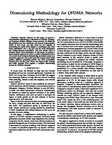
Comparison of CQN model with simulation.

would be greater than , in some sense such as the mean. Of course, by design the CQN does not distinguish between these two cases, and assumes that the former pertains. Thus, it is of interest to compare the CQN model with simulated scenarios where the TCP is working well and where it is not. is For all of the simulations in [3], the mean idle time assumed to be 5 s, and the mean file size (including overhead) is 200 K bytes. Thus, in the CQN model, the mean service time is 1.0667 s ( divided by the link speed of at the PS node 1.5 Mb/s). The number of sources is either 25 or 50. This then in the CQN model (1). Further specifies the distribution for pertinent aspects of the simulation include the assumption that the buffer feeding the T1 links is served FIFO and the choice of buffer management strategy; when the buffer is full and an additional packet arrives, discard: 1) the new packet; or 2) the oldest packet, i.e., the packet at the front of the queue. Heyman et al. also consider different distributions for the idle times and the file sizes, including the Pareto distribution. The simulations show that these distributions influence the distribution of only via their means, as predicted by their Engset models, as well as the CQN herein. Fig. 2 shows the pmf for five of the scenarios in the CQN considered in [3], as well as the prediction for model. The five scenarios have various combinations of deterministic, exponential, and Pareto distributions for the file sizes and idle times, as well as discard policies of drop-from-front and drop-from-tail, and they all have 50 sources. Note that the prediction from the CQN model is close to three of the scenarios. These three scenarios have a TCP degradation factor of between 0.95–0.99, where this factor in the Heyman et al.model captures “the performance impairment due to TCP not accurately tracking the bottleneck link rate,” and whose ideal value is 1. Thus, in these three scenarios, TCP is working excellently, and the match to the CQN model is surprisingly good. In contrast, the two remaining scenarios consider TCP/IP running over ATM and the TCP degradation factor is 0.80. As expected, the number of active sources increases (the distribution shifts to the right) and the CQN model is no longer a good match. Note however that from the viewpoint of dimensioning, since there are more active sources than there are sources with bytes queued at the bottleneck link, those sources that do have bytes queued will still be receiving (better than) the bandwidth objective for which

the link was dimensioned. Of course, some users are nevertheless obtaining a degraded goodput, but the cause is primarily the interaction of TCP with ATM and buffer size and buffer management policy. This degradation in throughput ought to be corrected by improvements in TCP and/or in ATM layer controls. B. Accuracy of Asymptotic Approximations Table I illustrates the accuracy of the “ -Poisson” approximation, the asymptotic approximation (21), the first term of (21), and the normal approximation. For various numbers of sources , and for chosen so that the PS node is relatively heavily loaded, the quantile was then chosen so that the exact tail probability is around 0.01. Note that although is greater is finite; see Section III for than 1, the CQN is stable since further discussion. Table I gives the percent error in the approxi), as compared with the exact calmate calculation of Pr( for culation. The “ -Poisson” approximation uses the partition function H(N), (3), and is clearly the most accurate approximation of the four listed. The asymptotic approximation for and in addition approximates (21) also uses the summation in (1). Table I shows that the asymptotic approximation (21) is qualitatively closer to the exact calculation than is the first-term alone of the asymptotic approximation (21). The normal approximation gives a rather poor estimate of the tail probability for these parameter values, although, as illustrated in Fig. 3, the overall match to the pmf appears reasonable, even . In any case, as shown and discussed for the case of in the subsequent sections, the bandwidth dimensioned via the normal approximation is rather close to the correct value. Fig. 4(a) and (b) illustrate the relative accuracy of the approximations for two of the cases in Table I. For a relatively few , Fig. 4(a) visually shows that the correction sources, term (the second term) in (21) significantly adds to the accuracy , of the approximation. For a larger number of sources, Fig. 4(b) shows that the asymptotic approximation is accurate to . tail probabilities as small as C. Impact of Choice of Performance Criterion As compared with the mean criterion, the increased tightness of the tail criterion impacts the dimensioning rule (32) via the parameter , which in turn depends on , the (1– )-quantile of a Normal(0, 1) random variable. Note that in the case of the normal approximation, the mean performance criterion


651

Fig. 3. Probability mass function for # at PS node, and associated normal 25, = = 10. approximation.

N=

TABLE II REQUIRED BANDWIDTH, FOR GIVEN NUMBER OF SOURCES N , WHERE f = b = 100 Kb/s. THE PERCENTS NOT-IN-PARENTHESES ARE FROM THE EXACT CALCULATION OF BANDWIDTH, WHILE THE PERCENTS IN PARENTHESES ARE FROM THE NORMAL APPROXIMATION, PROPOSITION 1, (31) AND (32)

is given by the 50% quantile, i.e., when is zero. Table II illustrates the increase in the required bandwidth as decreases. The key observation is that although tighter performance criteria (smaller values of ) increase the required bandwidth the percentage increase is relatively minor for the relevant cases of a few hundred sources. This is evident from (32) where and the square-root term is dominated by the linear term of , for large . Heuristically, one would expect this, since the is fairly concentrated around the mean; see Fig. 2. pmf for and Moreover, in the asymptotic limit where (many sources and fast service at the PS node), the becomes a single point mass. Thus, the distribution of model suggests that a network operator can design for a rather strong-sounding objective—with 99% probability the per-flow throughput is greater than a threshold—without requiring the deployment of much more bandwidth than for an objective on

(a)

(b) Fig. 4. (a) Comparison of asymptotic approximations with exact calculation, for N = 25, = 2:5. (b) Comparison of asymptotic approximations with exact calculation, for N = 100, = 3:33.

the mean. If the network operator also implements a connection admission control (see Section V), then the design objective could be strengthened to be a service objective. Also note that the percentage increase based on the normal approximation is close to that from the exact calculation. This is due to the fact that the normal approximation describes devi. ations from the mean of the order of If a network operator would like to use the tail performance criterion, but would prefer a simpler dimensioning rule than (32), then the dimensioning rule for the mean criterion could

652


TABLE III RATIO OF FULL ALLOCATION TO ENGINEERED BANDWIDTH, N 1000, AND = 0:01

=

N b=B , FOR

again be used with a larger value of the effective bandwidth parameter , where this increase is chosen to bound the percentage increases for parameter values of interest, such as in Table II. D. Comparison to Full Allocation of Bandwidth It is instructive to compare the engineered bandwidth with what would have been required if a full allocation of the sources. per-flow objective were provided for each of the , the equation (35) becomes Setting (37) . As is typically small, is roughly a simple hyperbola in . For an analogous viewpoint, one can define the “statistical gain” to be the ratio of the full allocation of bandwidth to the engineered bandwidth, . For the mean performance criterion, is approx. For a numerical example, Table III shows imately the statistical gain, given the tail performance criterion with and , for various values of and . For the given parameter values, is greater than one, and the normal approximation pertains. For comparison, the engineered bandwidth is computed both iteratively using (1) and via the normal approximation (32). As shown in Table III, the normal approximation is quite close to the exact numerical computation. Also, is small, but is the statistical gain is minor when the ratio . significant when is the throughput a source would obtain asRecall that suming the target link is not constraining the flow. Note that is determined by the constraints of other network components and includes the idle times at the source, whereas the per-flow bandwidth objective applies only during active periods of file transfers. Thus, a service provider could reasonably choose a bandwidth objective that is equal to or greater than . When is larger than , the service provider can realize significant savings in the engineered bandwidth as compared with the full allocation. where

VII. CONCLUSION We have derived simple and robust engineering rules for dimensioning bandwidth for elastic data traffic for a single bottleneck link. The derivation is based on normal approximations

for a CQN model in heavy traffic. For a mean performance criterion, we obtain the effective bandwidth of an elastic data source. We believe that simple ballpark dimensioning rules are appropriate because of the uncertainty in the forecasts of the traffic demands. The robustness of the dimensioning rules follows from the insensitivity property of the CQN model, whereby the distribution of the underlying random variables is pertinent only via the mean, and of particular interest, the mean of the file-sizes, and not their heavy-tail characteristics. We compared our CQN with simulations of file transfers regulated by TCP. Despite the simplicity of our CQN model, it accurately predicted the distribution for number of active sources at the bottleneck link, given the condition that the feedback control was performing well. The dimensioning rules satisfy a performance measure based on the mean or the tail-probability of the per-source bandwidth. In the case of the mean performance measure, the dimensioning rule has the linear effective-bandwidth form. For the tail performance measure, the dimensioning rule is still in closed-form, though no longer linear in the number of sources. If the network designer wishes to use a linear rule for the sake of simplicity, then the dimensioning rule for the mean criterion could again be used with an increased value of the effective bandwidth parameter, where the increase is estimated for parameter values of most interest. The dimensioning rules are easily inverted to obtain the number of sources that can be supported on a link of given bandwidth. We illustrated the increase in bandwidth needed to satisfy the tail performance objective as compared with the mean objective. The key observation is that although tighter performance criteria increases the required bandwidth, the percentage increase is relatively minor, particularly for the relevant case of at least a few hundred sources. This occurs since the pmf of is rather concentrated around the mean. Thus, the model suggests that a network operator can design for a rather strong-sounding objective—with 99% probability the per-source throughput is greater than a threshold—without requiring the deployment of much more bandwidth than for an objective on the mean. We also showed regimes where statistical gain can and cannot be realized. We provide a new derivation of the normal approximation in CQNs using more accurate uniform asymptotic approximations and give an explicit estimate of the error in the normal approximation. For the region of applicability, the uniform asymptotic expansion is accurate to within a few percentage points, and the “ -Poisson” approximation is accurate to within a tenth of a percentage point. Although the normal approximation is less accurate than the other approximations, the bandwidth dimensioned based on this approximation is rather close to the correct value in the region of interest of some hundreds of sources, as , is then relatively the pmf for the number of active sources, concentrated around the mean. The present work has focused on a single bottleneck link and a single class of traffic. The generalization to multiple classes is examined in [30] and [31]. In future work, we intend to extend the results to derive dimensioning methods for general network topologies and multiple classes of elastic traffic. The methods will depend on additional asymptotic results.


where

APPENDIX PROOF OF LEMMAS Proof of Lemma 1: The idea of the proof is to determine , (3), and then use the an asymptotic approximation for relation (A.1) is given in (3) and . For , where is a particular case of the asymptotic approximation for (16) in [27]. To apply (16) of [27], note that the -transform of is , and from the inverse Cauchy forcan be expressed as mula,

In the notation of [27], , . From (16) in [27], for and

653

where and

(A.6) , denoted , is , and the nonzero The saddle point of . From the condition of pole of the integrand in (A.4) is for some constant Lemma 2 that , we know that the saddle point is less than the pole 1, and becomes small for large . Thus we that the difference need the uniform asymptotic approximation given by (17) in the preliminaries of [27]; from which one obtains

(A.7)

, and

(A.5)

and

where (A.2)

(A.8)

, which is negative for and where in (16). Lemma 1 follows from (A.2) and (A.1). equals , (1), and for Proof of Lemma 2: From the pmf for

equals the right-hand From (14), (15) note that side of (A.8). Substituting (A.7) into (A.3) yields (21) of Lemma 2. ACKNOWLEDGMENT The authors would like to thank D. Heyman for the simulation results from his joint studies with T. Lakshman and A. Neidhardt. They also would like to thank W. Whitt for his thoughtful comments on a prior draft of this paper, and to the anonymous reviewers for their constructive suggestions. REFERENCES

where and

is given in (3). From the conditions of Lemma 2 that , can be replaced with (A.2) yielding (A.3)

The remainder of the proof is to obtain the uniform asymptotic . The -transform of the parapproximation for is tition function

Following [27], and using the inverse Cauchy formula, we have

(A.4)

[1] S. Lavenberg, Ed., Computer Performance Modeling Handbook. New York, NY: Academic, 1983. [2] I. Mitrani and E. Gelenbe, Analysis and Synthesis of Computer Systems. New York, NY: Academic, 1980. [3] D. P. Heyman, T. V. Lakshman, and A. L. Neidhardt, “A new method for analyzing feedback-based protocols with applications to engineering web traffic over the internet,” in Proc. ACM SIGMETRICS’97, Performance Evaluation Rev., vol. 25, 1997, pp. 24–38. [4] V. Paxson and S. Floyd, “Wide-area traffic: The failure of Poisson modeling,” IEEE/ACM Trans. Networking, vol. 3, pp. 226–244, 1995. [5] W. Willinger, M. S. Taqqu, R. Sherman, and D. V. Wilson, “Self-similarity through high variability: statistical analysis of ethernet LAN traffic at the source level,” IEEE/ACM Trans. Networking, vol. 5, pp. 71–86, 1997. [6] A. Varma and D. Stiliadis, “Hardware implementation of fair queueing algorithms for ATM networks,” IEEE Commun. Mag., vol. 35, pp. 54–68, Dec. 1997. [7] A. Berger, L. Bregman, and Y. Kogan, “Bottleneck analysis in multiclass closed queueing networks and its application,” Queueing Systems, vol. 31, pp. 217–237, 1999. [8] D. Bertsekas and R. Gallager, Data Networks, 2nd ed. Englewood Cliffs, NJ: Prentice Hall, 1992. [9] J. S. Kaufman, “Blocking in a shared resource environment,” IEEE Trans. Commun., vol. 29, pp. 1474–1481, 1981. [10] J. W. Roberts, “A service system with heterogeneous user requirements,” in Performance of Data Communications Systems and Their Applications, G. Pujolle, Ed. Amsterdam, The Netherlands: North Holland, 1981, pp. 423–431.

654

[11] D. Mitra and J. Morrison, “Erlang capacity and uniform approximations for shared unbuffered resources,” IEEE/ACM Trans. Networking, vol. 2, pp. 581–587, 1994. [12] C.-S. Chang and J. A. Thomas, “Effective bandwidth in high-speed digital networks,” IEEE J. Select. Areas Commun., vol. 13, pp. 1091–1100, Aug. 1995. [13] G. de Veciana, G. Kesidis, and J. Walrand, “Resource management in wide-area ATM networks using effective bandwidths,” IEEE J. Select. Areas Commun., vol. 13, pp. 1081–1090, Aug. 1995. [14] F. P. Kelly, “Notes on effective bandwidths,” in Stochastic Networks. Oxford, U.K.: Clarendon, 1996, pp. 141–168. [15] W. R. Stevens, TCP/IP Illustrated, Volume 1, The Protocols. Reading, MA: Addison-Wesley, 1994. [16] S. Floyd, “TCP and explicit congestion notification,” ACM Comput. Commun. Rev., vol. 24, pp. 10–23, Oct. 1994. [17] K. Ramakrishnan and S. Floyd, “A proposal to add explicit congestion notification (ECN) to IP,” Internet Engineering Task Force, Request for Comments 2481, Jan. 1999. [18] K. W. Fendick, “Evolution of controls for the Available Bit Rate service,” IEEE Commun. Mag., vol. 34, pp. 35–39, Nov. 1996. [19] A. Romanov and S. Floyd, “Dynamics of TCP traffic over ATM networks,” IEEE J. Select. Areas Commun., vol. 13, pp. 641–633, 1995. [20] C. Fang, H. Chen, and J. Hutchins, “A simulation study of TCP performance in ATM networks,” in Proc. IEEE Globecom’94, Nov. 1994, pp. 1217–1223. [21] H. Balakrishnan, H. Rahul, and S. Seshan, “An integrated congestion management architecture for internet hosts,” in ACM SIGCOMM’99, Cambridge, MA, 1999, pp. 175–187. [22] M. Schwartz, Telecommunication Networks: Protocol, Modeling, and Analysis. Reading, MA: Addison-Wesley, 1986. [23] A. E. Ferdinand, “An analysis of the machine interference model,” IBM Syst. J., vol. 10, pp. 129–142, 1971. [24] B. Pittel, “Closed exponential networks of queues with saturation: The Jackson-type stationary distribution and its asymptotic analysis,” Math. Oper. Res., vol. 4, pp. 357–378, 1979. [25] M. Friedlin and A. Wentzell, Random Perturbations of Dynamical Systems. New York, NY: Springer-Verlag, 1984. [26] A. Birman and Y. Kogan, “Asymptotic evaluation of closed queueing networks with many stations,” Commun. Statistics, Stochastic Models, vol. 8, pp. 543–564, 1992. , “Error bounds for asymptotic approximations of the partition [27] function,” Queueing Syst., vol. 23, pp. 217–234, 1996. [28] Y. Kogan and M. Shenfild, “Asymptotic solutions of generalized multiclass Engset model,” in Proc. 14th Int. Teletraffic Cong.—The Fundamental Role Teletraffic in the Evolution of Telecommunications Networks, J. Labetoule and J. W. Roberts, Eds, 1994, pp. 1239–1249.


[29] F. P. Kelly, “Loss networks,” Ann. Appl. Probability, vol. 1, pp. 319–378, 1991. [30] A. W. Berger and Y. Kogan, “Multiclass elastic data traffic: Bandwidth engineering using asymptotic approximations,” in Proc. 16th Int. Teletraffic Cong.—Teletraffic Engineering in a Competitive World, P. Key and D. Smith, Eds, 1999, pp. 77–86. , “Distribution of processor-sharing customers for a large closed [31] system with multiple classes,” SIAM J. Appl. Math., vol. 60, pp. 1330–1339, 2000.

Arthur W. Berger (S’82–M’83–SM’97) received the Ph.D. degree in applied mathematics from Harvard University, Cambridge, MA, in 1983. He joined AT&T Bell Laboratories and subsequently AT&T Labs in 1996 and Lucent Bell Labs in 1998. Currently, he is a Senior Research Scientist with Akamai Technologies, Cambridge. His research interests include: content delivery over the Internet, predicting Internet performance, design and performance of high-speed data networks and equipment, quality of service in the Internet, IP over optical transport networks, traffic engineering, congestion controls, stochastic models.

Yaakov Kogan (SM’91) received the Candidate of Sciences (the Soviet equivalent of the Ph.D. degree) and Doctor of Sciences degrees from the U.S.S.R. Academy of Sciences in 1968 and 1987, respectively. He is a Principal Technical Staff Member at AT&T Labs, Middletown, NJ, where he works in the Network Design and Performance Analysis Department. After receiving the Ph.D., he worked on performance analysis of computer and communication systems and developed nonparametric and asymptotic methods for solving stochastic models of large dimension. His recent activities include performance and reliability analysis of corporate IP backbone networks. Dr. Kogan is a member of IFIP Working Group on Computer System Modeling.