Direct simulations and modelling of basic three ... - CiteSeerX

c 2004 Cambridge University Press J. Fluid Mech. (2004), vol. 519, pp. 1–32.
DOI: 10.1017/S0022112004000606 Printed in the United Kingdom

1

Direct simulations and modelling of basic three-dimensional bifurcating tube flows By M. T A D J F A R1,2 1

AND

F. T. S M I T H3

Advanced Computing Center, Institute of Physical and Chemical Research (RIKEN), 2-1, Hirosawa, Wako-shi, Saitama, 351-0198, Japan 2 Department of Aerospace Engineering, Amir-Kabir University, Tehran, Iran 3 Department of Mathematics, University College London, Gower Street, London WC1E 6BT, UK

(Received 5 February 2003 and in revised form 5 May 2004)

Three-dimensional bifurcating internal flow is studied for a single mother tube branching into two equal but diverging daughter tubes. The mother tube is straight and of circular cross-section, containing a fully developed incident motion, while the diverging daughters are straight and of semi-circular cross-section. This basic configuration is treated first by direct numerical simulation and secondly by slenderflow modelling, for a variety of Reynolds numbers and angles of divergence. The direct simulations and modelling highlight different forms of three-dimensional separation or flow reversal as well as enhanced upstream and downstream influence and pressure loss induced by the bifurcations especially at increased divergence angles. Comparisons between the results from the simulations and those from the slender-flow modelling show relatively close agreement at medium values of Reynolds number. In particular, as the angle of divergence increases for a given Reynolds number, there is generally first an increase in flow attachment on to the inner divider wall(s) and then, at higher angles, an increasing trend to flow reversal at the corners formed by the junctions of the outer wall with the divider; longitudinal vortex motion is also enhanced then. The agreement persists over a surprisingly wide range of divergence angles.

1. Introduction The most common cases of internal-flow branching studied theoretically, computationally, experimentally and observed in reality are those of one-to-two branching, where one mother tube flow feeds into two daughter tube flows downstream. In three-dimensional motion, which is the major practical concern for biomedical flows in particular (Pedley 1980; Caro et al. 1996, for example), theoretical studies include those by Pedley, Schroter & Sudlow (1970, 1977), Smith (1976a, 1977), Bennett (1987), Blyth & Mestel (1999), Smith & Jones (2000). In two-dimensional branching channel models, Smith (1976b), Badr et al. (1985), Brotherton-Ratcliffe (1987) and Smith et al. (2003b) are among the theoretical works. Most such investigations adopt approximations or asymptotic analyses appropriate to relatively high flow rates, whereas Tutty (1988) considers low flow rates. More realistic models with various degrees of accuracy for aortic or carotid branchings are examined by Roach, Scott & Ferguson (1972), Motimoya & Karino (1984), Fisher & Fieman (1990) (see also Augst 2003) and for early generation branches of the cardiovascular and lung systems by Lighthill (1972). A wide scatter of branching-flow conditions is covered by theory and, especially recently, by direct numerical simulations. Simulations include those of Roach et al.,

2

M. Tadjfar and F. T. Smith

Motimoya & Karino, Fisher & Fieman above, as well as Bramley & Dennis (1984), Gatlin et al. (1995), Zhao, Brunskill & Lieber (1997), Corieri et al. (1991), Lei, Kleinstreuer & Archie (1997), Comer, Kleinstreuer & Zhang (2001). In particular, Comer et al. address three-dimensional steady laminar branching motion of incompressible fluid through two successive bifurcations in a rigid smooth tube. Planar branching motion is examined by Bramley & Dennis and Wilquem & Degrez (1997), the latter for two successive symmetric bifurcations. Tadjfar & Himeno (2002a) have developed a time-accurate solver to study the flow into branches. The solver is capable of handling moving grids and boundaries in complex three-dimensional geometries. The code has been validated by performing a series of numerical simulations. The results of these simulations, representative of typical biological flows, compare favourably with theoretical and experimental results according to Tadjfar, Yamaguchi & Himeno (2000) and Tadjfar & Himeno (2001). The width of coverage by theory and simulations reflects the prevalence of branchings in the human body and the variety of haemodynamic conditions, for example, in terms of Reynolds number, wall compliance, branching non-symmetry and unsteadiness. Networks of successive one-to-two branchings have also been studied, as is clear from some of the papers above. Network studies to date tend to simplify the flow at individual branchings or restrict attention to a small number of generations. Another type of network in effect is provided by one-to-many branchings, studied by Hademonos, Massoud & Vinuela (1996), Gao et al. (1997), Smith & Jones (2000, 2003) and motivated by the haemodynamics of arteriovenous malformations in the brain. Such a one-to-many network may itself form a significant part of a larger intracranial network, however. Other related basic aspects of branching here are to be found in Pedley (1977, 1980), Snyder, Dantzker & Jaeger (1981) and Corieri et al. (1991). Again, aspects of the work by Pedley and Pedley et al. (1977) are incorporated in models for lung airways assuming symmetric branchings: see also the Weibel model, Wilquem & Degrez (1997), Comer et al. (2001). The typical Reynolds numbers of interest are of medium value, in the hundreds or low thousands at most, with branching flows usually remaining laminar (see e.g. Pedley 1977; Pedley et al. 1977). Quasi-steadiness and the interplay between inviscid and viscous effects acting over different length scales are also estimated by Pedley (1977, 1980) and Smith & Jones (2000, 2003). Comparisons in recent studies show that in many branching configurations there is fairly strong agreement between slender-flow theory and direct numerical simulations, either in a quantitative sense for medium flow rates or qualitative at lower flow rates. Thus, the local theory in Smith & Jones (2000) for multi-branching in the presence of small pressure differences agrees with the direct simulations of Wilquem & Degrez (1997) in the special case of two successive one-to-two branchings over a range of Reynolds numbers from 200 to 1200. The local-global theory in Smith and et al. (2003b) and Smith (2002) for side-branching agrees with direct simulations at Reynolds numbers of about 200 or above, explaining the pressure-jump phenomena found in the simulations, a jump which is different dynamically from others identified earlier. The theory in Smith & Jones (2003) of multi-branching using multiple nonlinear recurrence relations, but with sizeable pressure differences, agrees quite well quantitatively with subsequent direct simulations (Smith et al. 2003a; Bowles et al. 2004) for Reynolds numbers beyond 50. Results from slender-flow theory in Smith et al. (2003a) for three-dimensional straight bifurcations agree with simulations at Reynolds numbers of 20 and beyond. These cover various one-to-two or one-to-many branchings, in two-dimensional and three-dimensional configurations. The divergence

Direct simulations and modelling of bifurcating tube flows (a)

3

(b) u z y, n s α

z β α n

z

β

y s x

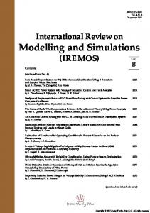
Figure 1. (a) Diagram of mother tube with circular cross-section bifurcating into semicircular daughter tubes, diverging at angles α, β, and of coordinates x, y, z, s, n used. (b) Top view.

angles observed in the respiratory, cardiovascular and cranial systems of the body vary considerably, from zero to 180◦ approximately, over the wide range of sites present, while the typical Reynolds numbers also vary, but up to a maximum value of a few thousand. It seems clear, then, that both theoretical modelling and direct simulations can be beneficial here. Rather complex fluid dynamics is involved, especially with threedimensional effects active at a bifurcation, and considerable insight is needed, which can often be provided by comparisons between direct simulations and theoretical modelling. In addition, the coverage of parameter space by simulations and by theoretical approaches is wide but patchy so far, with simulations to date being unable to handle accurately more than a few generations of branching, so that modelling seems necessary or at least of potential help, while questions remain on how well modelling or approximation works in realistic configurations. Coverage over a range of parameters with benchmark results on basic branching problems is felt to be desirable. Present formulation Three-dimensional laminar steady flow of incompressible viscous fluid through a straight mother tube bifurcating into two straight but divergent daughters tubes is to be considered here. The mother is of circular cross-section with radius aD and the daughters, after a local adjustment near the bifurcation point, are of semi-circular cross-section. The angle between the longitudinal axis of one daughter (the right-hand one) and the mother axis is prescribed as α and between the other daughter axis and the mother axis is β, the three axes being coplanar. Our interest throughout this paper is in the basic case of α, β being equal, so that α then represents half the angle of divergence, and in left–right flow symmetry (see figure 1). Fully developed flow with a given mass flux is assumed sufficiently far upstream in the mother. Non-dimensional velocity components u ≡ (u, v, w,), corresponding to Cartesian coordinates (x, y, z) (with x longitudinal and y, z cross-sectional in the mother), and pressure p are used, respectively, based on a characteristic velocity scale uD , on aD and on ρD u2D where ρD is the fluid density. Hence, the continuity and Navier–Stokes equations take the form ∇ · u = 0, (1.1a) (u · ∇)u = −∇p + Re−1 ∇2 u.

(1.1b)

4

M. Tadjfar and F. T. Smith

Here, ∇ denotes the operator (∂x , ∂y , ∂z ), while Re ≡ uD aD /νD is the Reynolds number with νD denoting the kinematic viscosity of the fluid. The geometry of the bifurcating tube may be specified in terms of x, y, z or associated polar coordinates. Flow solutions for this basic configuration are obtained below by means of direct numerical simulation and slender-flow modelling, accompanied by comparisons between the two. Sections 2 and 3 describe in turn the direct numerical simulations which are based on a finite-volume approach and the slender-flow treatment which is based on the three-dimensional flow response over the longer length scales where full viscous–inviscid balances apply. The results are presented and compared quantitatively and qualitatively in § 4 over a range of Reynolds number Re and half divergence angles α. Shorter-scale behaviour, upstream and downstream influence, flow reversal (separation) and increased flow attachment are also examined. The final section, § 5, provides further discussion of the work. 2. Direct numerical simulations The unsteady version of the three-dimensional incompressible continuity and Navier–Stokes equations (1.1a, b) was solved using a parallel time-accurate finitevolume solver. The solver is capable of dealing with moving boundaries, moving grids and complex three-dimensional vascular systems. The computational domain is divided into multiple block subdomains. At each cross-section, the plane is divided into twelve sub-zones to allow flexibility for handling complex geometries and, if needed, appropriate parallel data partitioning. A second-order in time and third-order upwind finite-volume method for solving time-accurate incompressible flows based on pseudo-compressibility and a dual time-stepping technique is used. Performing a series of numerical simulations validated this code. The results of these simulations, representative of typical biological flows, have been compared previously with theoretical and experimental results, showing favourable agreement. In the numerical method, the equations in strong conservative form are written in a generalized curvilinear coordinate such that
system,

∂ q¯ ∂ ¯ v g ) · nˆ dS = 0, ¯ dV + ( f¯ − Q¯ (2.1) dV + Q ∂τ ∂t V (t)

V (t)

S(t)

¯+G ¯ v, H ¯+H ¯ v ) and ¯+F ¯v, G where f¯ = ( F       2  u u u +p     v   v  ¯  uv   ¯ ¯ Q =  , q =  , F =  ,    w w uw     0 p βu         wu vu    2  wv + p u      ¯ ¯  , , H=  2 G=      vw w +p   βw βv     2ux vx + uy    1 1 u + v 2vy       y x ¯ ¯ Fv = −   , G v = − ,  Re uz + wx Re vz + wy      0 0       wx + uz    1 w + v    y z  ¯ Hv = −   2w .   Re z  0

(2.2)

Direct simulations and modelling of bifurcating tube flows

5

Here, t denotes the real physical time, τ is the pseudo-time, and β is the pseudocompressibility coefficient, while V (t) is the time-varying volume of the cell, S(t) denotes the surface of the control volume and nˆ is the outward unit normal vector at the surface of the control volume, where v¯g is the local velocity of the moving control surface. The term q¯ associated with the pseudo-time is designed for an inner subiteration at each physical time step and vanishes when the divergence of velocity is driven to zero so as to satisfy the equation of continuity. For a structured boundary-fitted computational coordinate system (ξ, η, ζ ) and a cell-centred finitevolume formulation, we can write (2.1) in a semi-discrete form for each cell centred at points (i, j, k), ∂ ¯ ij k + R ¯ ij k + StVij k ∂ q¯ = 0. (2.3) St [V Q] ∂t ∂τ ij k Here, the steady-state residual is given by ˜+G ˜ v )i,j +1/2,k ¯ ij k = ( F˜ + F˜ v )i+1/2,j,k − ( F˜ + F˜ v )i−1/2,j,k + ( G R ˜+G ˜ ) ˜ ˜ ˜ ˜ − (G v i,j −1/2,k + ( H + H v )i,j,k+1/2 − ( H + H v )i,j,k−1/2 .

(2.4)

Also, the modified flux terms are defined as

 ¯ v¯g ) · ¯Sξ ,  F˜ + F˜ v = ( f¯ − St Q n   η ˜ ¯ ˜ ¯ ¯ G + G v = ( f − St Q v¯g ) · Sn ,   ζ  ˜+H ˜ = ( f¯ − St Q ¯ ¯ ¯ H v ) · S . v g n

The normal-area vector in the ξ -direction is   ¯Sξ = S ξ , S ξ , S ξ . nx ny nz n

(2.5)

(2.6)

In the above formulation, the flow Strouhal number is defined as St = D/(Uref tref ). The physical time derivatives are differenced using the second-order trapezoidal implicit method, while first-order Euler implicit differencing is used on the pseudotime derivatives. The inviscid fluxes are differenced using third-order upwind implementation of Roe’s flux-difference split averaging technique. Second-order central differencing is used on the viscous fluxes. To maintain second-order spatial accuracy, a special treatment at the boundaries is required. Boundary conditions At the inlet of the mother tube, a parabolic profile is assumed for the velocities, u = 1−(y 2 +z2 ), v = w = 0, with the reference velocity taken as the central (maximum) velocity, and ∂ss(p) = 0 is imposed on the pressure. Here, s is the local streamwise direction along the centreline of each tube. In the mother tube, s is the same as x, and in the daughter tubes, is along the angles α and β off the x-axis (see figure 1a); the bifurcation occurs at a station s = s0 , x = x0 , say. To fix the role of wall curvature on the issue of geometric transition between the daughter tubes and the mother tube, a very simple transition is considered. In this model, the daughter-tube radius is equal to that of the mother tube. Hence, we can envisage a circle with the radius of the mother tube, at the z = 0 cross-section, with the centre located along the apex of the bifurcation (see the dotted line in figure 1b). The outer walls of the right daughter tube intersect the outer walls of the mother tube along the half-angle line, α/2 (the large dashed line). The mother tube at the apex of the bifurcation is ten radii in

6

M. Tadjfar and F. T. Smith

Figure 2. Computational grid for the branch model with α = β = π/8.

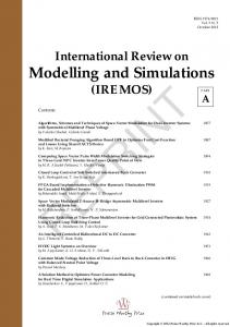
length, and at the outermost walls at y = 1 is shorter by aD tan(α/2). Since interesting physics may occur near the bifurcation region, we chose the cross-section along the large dashed line as our main point of reference with s(= s0 ) = 10. So as we move upstream along the centreline of the mother tube towards the entrance, we reach it at s = 0. Similarly, as we move downstream along the dividing plate in the inner walls of the daughter tubes, we reach the outlet at s = 20. We also define a local normal direction n which is defined as positive inwardly normal to the walls in all the tubes. This definition helps in evaluating the wall shear values at the tube walls. Therefore, n is always perpendicular to s. Both s and n are non-dimensionalized by the mother tube radius, of course. At the outlet of each daughter tube, the pressure is imposed as p = 0, while for the velocities ∂ss(u, v, w) = 0, a condition which is appropriate for the present pseudo-compressibility method. Along the rigid walls, the no-slip condition (u, v, w) = 0 is assumed. Grid independence Based on the branch model chosen here, numerical grids are generated that extend 10 main tube radii upstream and downstream from the bifurcation. Four grids of different grid density comprising 68 832, 113 616, 132 528, and 212 508 cells were considered. The high-density grid for the case with α = β = π/8 is shown in figure 2. The results were close in all cases for most of the flow, but in the peak values occurring near the bifurcation region they differed. The maximum difference in the peak values of the wall shear and wall pressure between the two highest-density grids considered here was less than 2%. Either grid produces grid-independent numerical results. However, for the aesthetic reason of presenting smooth graphs, the highestdensity grid was chosen for this study. In the mother tube, we use a 38 × 51 × 16 grid, which implies using 38 cells in the tube axial direction with 51 cells in the azimuthal direction and 16 cells in the radial direction at each cross-section of the tube. Similarly, in each of the daughter tubes, we use a 55 × 75 × 22 grid. Appropriate grid stretching near the walls in the radial direction and near the bifurcation region in the axial direction is implemented. For more detail on other aspects of the numerical technique see Tadjfar et al. (2000) and Tadjfar & Himeno (2001, 2002a, b). The results, denoted DNS, are presented in figures 3–12 and will be discussed in § 4 and compared there with those from the slender-flow model (SFM) which is considered next.

Direct simulations and modelling of bifurcating tube flows

7

3. Slender-flow model The slender-flow model is strictly for large Re values and mainly takes a long streamwise length scale |x − x0 | much greater than the cross-sectional ones (|y|, |z| of order unity), specifically a |x − x0 | scale of order Re. Shorter length scales which include upstream influence are considered later, particularly in Appendix A. On the present long length scale, the viscous filling of the tube flow takes place along with nonlinear inertial-viscous balancing, since then |u|, |y|, |z| are all of O(1), so provoking streamwise inertial forces (u∂u/∂x for example) and viscous forces (Re−1 ∂ 2 u/∂y 2 for example) of comparable order Re−1 . It follows that the typical angles of divergence of the bifurcation are assumed small and of order Re−1 , from the typical ratio of the |y|, |x − x0 | length scales. The flow solution then expands in the form ¯ + ..., (u, v, w) = (¯ u, Re−1 v¯, Re−1 w) −2 p = p¯ + Re p˜ + . . . ,

(3.1a) (3.1b)

with x − x0 = ReX. The coordinates X, y ,z are of order unity, as are the velocity and ¯, v¯, w, ¯ p. ˜ The velocity scalings stem from the continuity ¯ p, pressure contributions u ¯ balance, given the small angles present. The pressure contribution at leading order, p, likewise stems from the streamwise momentum scales, where the inertial and viscous terms are both of order Re−1 . The cross-sectional momentum balances, however, show ¯ ¯ that ∂ p/∂y, ∂ p/∂z must be zero, leaving ¯ p¯ = p(X),

(3.2)

an unknown function of X only. In consequence, the correction term p˜ must also be addressed. Here, p˜ remains dependent on y, z as well as X, since the cross-sectional inertial force is of characteristic size |u∂w/∂x| ∼ Re−2 , comparable with the pressure ˜ gradient |∂p/∂z| ∼ Re−2 (∂ p/∂z). Further, viscous diffusion is dominated by the y, z variation because the x variation is relatively small. Substitution of (3.1a, b),(3.2) into the continuity and Navier–Stokes equations (1.1) yields the controlling equations here as ¯X + v¯y + w ¯ z = 0, u

(3.3a)

¯ 2u ¯y + w¯ ¯, ¯u ¯X + v¯u ¯ uz = −p¯ (X) + ∇ u 2 ¯ v¯, ¯v¯X + v¯v¯y + w¯ ¯ vz = −p˜y + ∇ u

(3.3b)

¯ 2 w, ¯y + w ¯w ¯ z = −p˜z + ∇ ¯ ¯w ¯ X + v¯w w

(3.3d)

(3.3c)

¯ 2 denotes the dominant viscous operator (∂ 2 + ∂ 2 ), for the slender flow. Here, ∇ y z in line with the negligible influence of longitudinal diffusion. There is a clear nonlinear interplay of inertial, pressure-gradient and viscous forces coupled with vortex stretching mechanisms through the three-dimensional system. The system also contains a classical form of inviscid theory and classical lubrication theory as extremes, corresponding to inertial forces being relatively large or small, respectively. The appropriate boundary conditions on (3.3a)–(3.3d) are for no slip at the daughter tube walls in X > 0 and for the starting condition at X = 0. Here, X = 0 is the bifurcation point. Thus ¯ = v¯ = w ¯ X, ¯ = 0 at y = α ¯ X + (1 − z2 )1/2 and at y = α u

(3.4a)

¯ 0 ) at X = 0+, ¯ = (¯ (¯ u, v¯, w) u0 , v¯0 , w

(3.4b)

8

M. Tadjfar and F. T. Smith

¯ with the scaled angle α ¯ being of O(1). respectively, for −1 6 z 6 1. Here, α = Re−1 α ¯0 , v¯0 , w ¯ 0 are prescribed functions of y, z. The starting profiles u The starting position is just downstream of the bifurcation at X = 0+ for the ¯ > 0. Also, the total mass flux following reasons. The system is parabolic locally if u ¯ profile at an upstream station there is parabolicity is set; hence, given the input u globally as well. Upstream influence is absent on the present length scale provided that symmetry (equality) of the flows in the two daughters is maintained, in contrast with the effects of non-symmetry such as in Smith et al. (2003b). We then take it that there is no alteration to the tubewall circular cross-section, and hence no alteration to the original fully developed solution, ahead of the bifurcation point. Therefore, that ¯0 _ (1 − y 2 − z2 ), v¯0 = w ¯ 0 = 0 then. These solution holds for all X < 0. Moreover, u properties should be compared with those in Smith et al. (2003b) and elsewhere on global upstream influence. Finally here, the present long scale overlooks shorter length scales, principally x ∼ 1, where the flow solution has a mainly inviscid core and thin wall layers and exhibits upstream influence: see references in § 1. While short-distance analysis is helpful (see later) and lubrication limits may also be valuable at least in other contexts, the central slender-flow problem (3.3a)–(3.4b) is nonlinear and must, in general, be solved numerically. The numerical method used for (3.3a)–(3.3d) and (3.4a), (3.4b) is based on a Cartesian gridding approach to allow for general tube shapes and is described in Smith et al. (2003a). The wall conditions (3.4a) are transferred to the nearest grid point. The method overall can thereby be kept comparatively simple in terms of its differencing, but flexible in that many different cross-sections can be accommodated. With most streamwise varying cross-sections there is bound to be a degree of bumpiness within the numerical solution in the streamwise direction as some boundary points jump in or out of the domain from X station to X station, as well as in the cross-section itself. The major test on the influence of such bumpiness lies in examining the effects of grid refinement, and the influence is found to be small for the grids deployed in the present work. See further details below. The accuracy has also been checked in numerical terms by means of comparisons with fully developed and entry flows through tubes with circular or elliptic cross-sections, as well as in the approximation sense by comparisons with simulations in Smith et al. (2003a). Another feature is that analytical transformations are included in order to allow the centre of the grid to vary with X where necessary and the outer boundary of the grid to be expanded or contracted where appropriate, as X increases. In the present context, the ¯ X = y¯ , and velocity components transformation to (X, y¯ , z) coordinates, where y − α ¯, w) ¯u ¯ leaves in effect (3.4a) still holding, but at the walls and divider (¯ u, v¯ − α given by y¯2 + z2 = 1,

y¯ = 0,

(3.5a)

in turn, while the profiles in (3.4b) become ¯ 0 ) = (1, −¯ α , 0)(1 − y¯2 − z2 ). (¯ u0 , v¯0 , w

(3.5b)

Compare with Ahmad (1996). The governing equations remain (3.3a)–(3.3d) effectively ˜ ¯ y¯p¯ (X) instead of p. on use of p˜ − α The starting profiles (3.5b) are set at the station X = 0, then, on the grid, with p¯ set as zero at that station without loss of generality. At the next X station, the solution subject to semi-implicit differencing with uniform grid sizes X, ¯ y , z is obtained ¯ in the whole iteratively. First, p¯ is guessed; (3.3b) in difference form is solved for u

Direct simulations and modelling of bifurcating tube flows interior; the total mass flux

9



¯ d¯ u y dz

(3.6)

thus produced in difference form, integrated over the cross-section, is compared with the prescribed flux value (imposed by (3.5b)); and p¯ is adjusted to make ¯ in (3.4a),(3.5d) are incorporated the fluxes equal. The boundary conditions on u within the above iteration procedure. Secondly, (3.3a), (3.3c,) and (3.3d) are treated in a secondary-vorticity–velocity formulation. From those three equations and the ¯ y¯), we obtain the three equations definition ζ ≡ (∂¯ v /∂z − ∂ w/∂ ¯ 2 ζ − (¯ ¯z v¯X − u ¯y w ¯X , ¯ z) = u ¯X − ζu uζX + v¯ζy + wζ (3.7a) Re−1 ∇ ¯ 2 v¯ = ζz − u ¯Xy , ∇ ¯ 2w ¯Xz . ¯ = −ζy − u ∇

(3.7b) (3.7c)

¯ principally, but coupled through These are treated in turn as equations for ζ, v¯, w iteration. Differencing on (3.7a)–(3.7c) and successive solution throughout the interior of the grid is performed as for (3.3b). The boundary conditions on ζ are derived from ¯ y¯ , whereas those on v¯, w ¯ follow directly from the latest updated values of ∂¯ v /∂z, ∂ w/∂ (3.4a) with (3.5a). The iterations on (3.7a)–(3.7c) are continued until a convergence ¯ criterion on the maximum absolute differences between successive iterates for ζ, v¯, w is met. The approach overall is second-order accurate in the (¯ y , z)-cross-section apart from the wall-fitting effect. It is also made second-order accurate in the longitudinal direction by means of the double-stepping procedure described in Smith & Timoshin ¯ and so (1996). Further iteration involving use of (3.7a)–(3.7c) to update (3.3b) for u on can also be adopted. The procedure is repeated at each subsequent X station in marching fashion, with steps X. The typical grids used for SFM calculations have 121 × 121 points in the y¯ , z cross-plane and a step length X of 0.00001 (see also checks on the grid effects in the next section), although this varies from case to case: extra refinement proved necessary at the increased divergence angles referred to later. The results, denoted SFM, are presented in figures 3–9 where comparisons with direct simulations are also made, and these will be discussed in § 4, while Appendix B describes the asymptotes far downstream which are common to both the full and the slender-flow modelling and to all divergence angles. These asymptotes are (p, τ1 , τ2 ) ∼ (−10.56x/Re, 4.48, 3.84),

(3.8)

¯/∂ y¯ evaluated at z = 0 for y¯ = 0, 1 with τ1 , τ2 denoting the scaled wall shear stress ±∂ u in turn. 4. Results and comparisons Results from the simulations (DNS) and from the modelling (SFM), and comparisons, are presented together below. We are particularly interested in effects from increasing the divergence angles or the Reynolds number. The DNS computations were performed mainly for opening angles of α = β = 0, π/8, π/4, and π/3 at Re = 500. Several lines along the axial direction in the tubes are chosen to present the data; the centreline in the mother tube along the x-axis at y = z = 0, the outer wall in the mother tube defined as the line along the x-axis at y = 1 and z = 0, the outer wall of the right daughter tube (RDT) defined as the line along the axial direction (s-axis) at n = 1 and z = 0, and the inner wall of the right

10

M. Tadjfar and F. T. Smith

(a) (i) 0.6 Re = 500

0.5

Centreline MT

0.3

0

Outer wall RDT

0.2

Outer wall MT

p– – p– (0)

Pressure

0.4

Inner wall RDT

0.1

0

–0.1

–0.2

asy

–0.3 0

2

4

6

8

10

12

14

16

18

20

10

20 s

s (ii)

SFM o DNS, Re = 100 × DNS, Re = 500

40

downstream asymptote τ1

20

×

×O O

0

×

O

0.02 x

Figure 3(a). For caption see facing page.

daughter tube defined as the line along the axial direction (s-axis) at n = 0 and z = 0. Also, the corresponding values of αRe and (s − s0 )/Re, respectively, in the DNS runs ¯ and the X range in the parabolic SFM calculations, were used for the values of α which yield a predicted dominant pressure contribution p¯ and the two wall shear

11

Direct simulations and modelling of bifurcating tube flows (b) 1.2 Re = 500

1.0

0.6

Centreline MT

–0.1

Inner wall RDT p – p (0)

Pressure

0.8

0.4

0.2

–0.2 –0.3

Outer wall MT

asy Outer wall RDT

–0.4

0

10

15 s

0

2

4

6

8

10 s

12

14

16

18

20

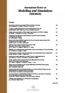
Figure 3. DNS and SFM results. (a) α = β = 0: (i) pressure distributions at Re = 500 (left DNS, right SFM) and (ii) wall shear at 100, 500 along the branched tube. (b) α = β = π/4, pressure at Re = 500 : DNS and SFM on left and right, respectively.

variations, τ1 , τ2 , along the centrelines of the divider and the semi-circular outer wall, as well as velocity profiles. The DNS and SFM results, with comparisons The pressure distributions along the axial direction according to DNS results are presented for the cases α = 0 and α = π/4 at Re = 500 in figures 3(a) and 3(b), respectively. The divider plane starts at s = s0 = 10 in all our cases. The non-axial variations in pressure are limited to the region near the bifurcation for the zero angle case. However, for the α = π/4 case, a small radial pressure gradient persists downstream owing to the (well known) existence of secondary flow generated by the bending of the axial streamlines. Also included in figure 3(a) for zero angle are the SFM results in the right daughter tube for pressure at Re of 500 and the wall shear stress (τ1 ) at Re of 100, 500, from both DNS and SFM, together with the downstream asymptotes. (We remark that here and below, the SFM and DNS results are usually shown with their axis scales being close if not quite identical; also ‘asy’ denotes the asymptote from (3.8)). In fact τ1 is plotted against X rather than s − s0 , and the DNS results at Re = 100, 500 are then seen to collapse well onto the unique SFM curve. The agreement is close overall in figure 3(a) and the approach to the downstream asymptote is relatively fast. In figure 3(b), which includes the SFM pressure for comparison at the increased angle π/4(¯ α = 125π), the agreement is reduced, as might ¯ value, but still remains remarkably close. The figure, in be expected at such a large α addition, shows grid effects (in the SFM pressure results from three different grids), which are seen to be quite small and indeed are barely discernible in the figure. The downstream asymptote is approached only slowly at the higher angle. The axial velocity profiles in the middle of the divider plate, z = 0, at different axial stations along the right daughter tube for α = 0 at Re = 100 are presented in figure 4(a) according to both DNS and SFM. Initially, we see the development of

12

M. Tadjfar and F. T. Smith (a) 1.0

1 s = 10.02 10.2 12.0 14.0 19.0

0.8

Re = 100

14.0

α=β=0

n 0.6

asy y

s = 10.2

0.4

0.2

0

0.5

1.0

1.5

0.4

0

Vaxial

0.8 u

1.2

1

(b) 1.0 s = 10.02 10.2 12.0 14.0 19.0

0.8

Re = 500 α = β = π/4

0.6

s = 12

y

n

14 19

0.4

asy

0.2

0

0.5

1.0

1.5

Vaxial

0

(c) 1

0.4

1 z=0

z=0

0

0.2

z=0

y

0.96

0.4

0.6 u

0.8

1.0 0

asy

s = 19

y

z = 0.96

1.2

1

s = 12

y

0.8 u

0.2

0.95

0.4

0.6 u

0.8

1.0 0

0.2

0.4

0.6

0.8

1.0

u

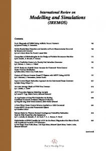
Figure 4. The axial velocity profiles (from DNS on left and SFM on right) in the centre of the divider plate of the right daughter tube with (a) α = β = 0 and Re = 100, (b) α = β = π/4 and Re = 500. Also shown in (c) are off-central as well as central profiles, from SFM for case (b), with s = 12, 19, asy.

a new boundary layer on the divider plane near the bifurcation at s = 10.02 and s = 10.2. For this Reynolds number, even at s = 12 the flow is close to the fully developed state, the profiles at stations s = 14 and s = 19 being almost identical. The DNS velocity profile data presented here are not at the actual grid nodes, but are

Direct simulations and modelling of bifurcating tube flows

13

the trilinear interpolation of the neighbouring cell centres. Hence the profiles are not as smooth as one would obtain from the actual computational nodes. Results from DNS and SFM nonetheless compare very favourably here. For the case with α = π/4 at Re = 500 in figure 4(b), again with DNS and SFM results, the flow never fully develops in our computational domain and we see the strong influence of the secondary flow in these axial velocity profiles. The secondary motion and its influence is gradually dissipated by the action of viscosity as the fluid moves downstream. The stations at s = 10.02 and s = 10.2 are very close to the bifurcation junction and a profile along the normal direction n would enter the mother tube rather than reaching the outer walls of the right daughter tube. This may well account for the differences in DNS and SFM velocities seen in parts of the profiles at some stations s, although the behaviour near the walls and near the maximum centreline velocities are clearly very ¯ = 125π, includes similar. Figure 4(c), which is likewise for α = π/4, Re = 500, giving α SFM velocity profiles for non-zero (off-central) z values at three stations s = 12, 19, ∞ in effect, this last being from the asymptote given in Appendix B. Each of the three plots has z values equi-spaced between z = 0 and 0.96 or, in the asymptotic case, 0.95, the slight difference being due to the grid methodology described in § 3. The methodology also explains why some neighbouring velocity profiles reach identical ¯ is zero at the curved outer wall. The profiles at s = 12, 19 along y¯ values where u with a comparison with the asymptotic profiles indicate the effective loss of mass flux near the centre which is counterbalanced, however, by significant gains (longitudinal vortex motions) in the off-central and near-corner flows. In contrast with the case of ¯ value is reduced and, in zero angle, moreover, in the π/4 case, the maximum u or u fact, two maximal positions occur, on either side of the symmetry plane, owing to the enhanced longitudinal vortices. The wall shear on the divider remains high, but the positions of maximum u at each z location are shifted away from the divider wall in ¯ (and those at the comparison with those upstream for the same divergence angle α ¯ ). The flow at s = 12, 19 is far from being fully developed. same distance but smaller α The Reynolds number influence on this can be observed in figures 5(a) and 5(b). At s = 19, far from the bifurcation, the fully developed state is delayed when Re is increased, as would be expected. However, at s = 10.02, near the bifurcation junction, the velocity profiles seem to converge as Re is increased. From these figures, we see that the influence of Reynolds number on the flow near the wall is far less than in the interior. We can also see a mild increase in the axial wall shear stress as Re is increased in figure 6 for the case with α = π/8. Concerning more detail of what happens as the bifurcation angles α and β are increased, the pressure distributions (DNS) along the centreline of the mother tube, presented in figure 7(a), demonstrate the upstream influence, where, in particular, the inlet pressure is increased as the bifurcation angle is widened: here α = β = 0, then π/8, π/4, π/3, following the direction of the arrow in this and subsequent figures Since the outlet pressure is kept at a constant value of p = 0 in both daughter tubes, this is just a manifestation of the higher pressure gradient required to drive the flow at constant Re = 500. This higher pressure gradient has to balance the higher energy losses in the more complicated flow in the bifurcation region and the further dissipation of the stronger secondary flow downstream from it. Pressure distributions along the inner wall of the right daughter tube, downstream of the bifurcation junction, are given in figure 7(b) from DNS and SFM. At this moderate Reynolds number, the nonlinear pressure gradient region looks limited fairly close to the bifurcation and for much of the tube we observe an almost linear pressure gradient even for relatively high values of α. The pressure drop, or loss, increases

14

M. Tadjfar and F. T. Smith (a) 1.0 Re = 20 100 255 500 764

0.8

s = 10.02 α = β = π/8 0.6 n 0.4

0.2

0

0.5

1.0

1.5

(b) 1.0 Re = 20 100 255 500 764

0.8

s = 19 α = β = π/8 0.6 n 0.4

0.2

0

0.5

1.0

1.5

Vaxial

Figure 5. For varying Re, the axial velocity profiles in the middle of the divider plate of the right daughter tube, from DNS, with (a) α = β = π/8 and s = 10.02, (b) α = β = π/8 and s = 19.

monotonically and significantly with α, however, and so does the typical downstream influence distance, as comparisons with the common asymptote indicate. We note that the SFM pressure curves are shown equated at the exit of the daughter, for the sake of comparison, and the DNS and SFM results broadly agree again. Further, higher Re values elongate the nonlinear region. We also examine the gradient of the axial velocity at the wall in the surface normal direction, ∂Vaxial /∂n (≡ τ1 ), which represents the normalized axial wall shear. This parameter is important both biologically, where many theories on the formation of vascular diseases are related to it, and physically since, as the velocities at the rigid

15

Direct simulations and modelling of bifurcating tube flows 50 Re = 20 100 255 500 764

40

dVaxi/dn

30 Inner wall RDT 20

10

0 10

11

12

13

14

15 s

16

17

18

19

20

Figure 6. The axial wall shear profiles along a line in the middle of the divider plate of the right daughter tube, from DNS, with α = β = π/8.

wall are zero, a negative value for wall shear indicates a region of back flow at that location. The axial wall shear distributions along the inner wall of the right daughter tube for different bifurcation angles at Re = 500 are presented in figure 8(a), from DNS and SFM again. Away from the bifurcation in the far downstream region, s & 13, we see a higher value of the axial wall shear as α is increased. This is due to the presence of a stronger secondary flow and its slower dissipation downstream. The enhanced downstream influence is re-emphasized here as α increases, whereas at low α, the approach to the downstream asymptote is quite rapid. Grid effects on τ1 (and on τ2 which varies much less than τ1 in general) obtained from the original first-order ¯ value of 125π associated with α = π/4, Re = 500, marching scheme, at the high α ¯ values, while are also shown in the figure to indicate the accuracy at such high α the DNS–SFM favourable comparison is broadly continued. The secondary flow action referred to above is even stronger in the near downstream region where the enhancement of axial wall shear owing to increasing α is even greater. However, an interesting feature occurs in the approach (upstream) to the leading edge of the divider plane. In figure 8(b), as α is increased, the axial wall shear actually decreases during the approach to s = 10. This suggests a trend to flow separation there in the case of α > π/2 say, that is, for a reversing bifurcation. Concentrating more on the axial wall shear along the outer wall of the right daughter tube as α is increased, these axial wall shear distributions (∂Vaxi /∂n and τ2 ) are presented in figure 9(a) from both DNS and SFM. The results are of the same order of magnitude throughout and although there are certainly differences in detail as the divergence angle is varied, the results confirm the lowness of the variation of τ2 compared with that of τ1 , especially away from the bifurcation. In the far downstream

16

M. Tadjfar and F. T. Smith (a) 0.9

0.8 Re = 500

Pressure

0.7

0.6

0.5

0.4

0.3

0.2 0

1

(b) 1.2 1.1 1.0 0.9 0.8 0.7 0.6 0.5 0.4 0.3 0.2 0.1 0

2

3

4

5 s

8

9

10

p – p (end)

0.5

0.1

10 11 12 13 14 15 16 17 18 19 20

7

0.9

Re = 500

Pressure

6

asy 10

s

20

s

Figure 7. For various α. (a) The pressure distributions along the centreline of the mother tube with Re = 500, from DNS. (b) The wall pressure distribution along a line in the middle of the divider plate of the right daughter tube with Re = 500: left DNS, right SFM.

region, the DNS axial wall shear is initially decreased as α is increased. However, this trend is reversed as the induced secondary flow becomes stronger at higher values of α. In the near bifurcation region, the decrease in axial wall shear continues into the formation of a separation bubble as the bifurcation angle is further increased. Similarly to the behaviour at the inner wall, the decreasing trend in axial wall shear values upstream is reversed during the approach to the bifurcation region, s = 10, as shown in figure 9(b). A cross-sectional shape of the separation bubble on the outer walls of the right daughter tube can be seen in the axial velocity contour distributions given in figure 10 for α = π/3 at Re = 500 and s = 10.3, just after the bifurcation.

Direct simulations and modelling of bifurcating tube flows (a) (i) 70

17

70

60 Re = 500

dVaxi/dn

50 40 τ1 30 20 10 0 10 11 12

13 14 15 s

16 17

18 19

20

0 10

20

s

(ii) 80

60

40

τ1 20

τ2

0

X

0.01

Figure 8(a). For caption see next page.

As the mother tube is being split into two daughter tubes, a dividing surface (wall) is created in the middle of the mother tube, the wall consisting of the straight divider planes in the simple model used here. The upstream influence from this wall is most keenly felt close to the top and bottom walls of the mother tube just before the bifurcation region. We can examine that upstream influence numerically by means of the axial wall shear distribution along a line in the middle of the upper wall of the mother tube which is the line in the x-direction at z = 1 and y = 0. (Analytically the upstream influence is described in Appendix A.) This axial wall shear distribution at Re = 500 is presented in figure 11. As the bifurcation angle is increased, the magnitude of the axial wall shear is decreased. The trend is accelerated nonlinearly by further increases in α and results in a strong backflow region at higher values of α. Again,

18

M. Tadjfar and F. T. Smith (b) 70

60

Re = 500

dVaxi/dn

50

40

30

20

10

0 10.0

10.1 s

10.2

Figure 8. (a) The axial wall shear profiles ((i) DNS–SFM comparison, (ii) SFM τ1 and τ2 versus X) along a line in the middle of the divider plate of the right daughter tube with Re = 500, for various α. (b) Close-up (DNS).

a cross-sectional shape of the separation region on the upper and lower walls of the mother tube just ahead of the bifurcation can be seen in the axial velocity contour distributions given in figure 12 for α = π/3 at Re = 500 and s = 9.9. Follow-up comments Reviewing the results of figures 3–12 as a whole, the major features as the divergence angle increases up to π/4 or π/3, apart from the qualitative or quantitative DNS–SFM comparisons, are the increasing downstream influence, the strengthening longitudinal vortices formed as the secondary flow increases, the axial velocity profiles becoming more complex, the short-scale effects growing, the rise of the wall shear stress τ1 and the increase in the pressure loss. This is especially so in each daughter tube. The increase of downstream influence and related features are seen first in comparing zero or low α results with the high α ones. At zero α (in figures 3a, 4a, 7, 8a, 9a), the development length is seen to be relatively short, as the flow is not far from fully developed at the X value of 0.02 corresponding to s − s0 = 10 for an Re of 500. (Although our prime concern is with non-zero α and/or with nonlinear effects, the good qualitative agreement with Blyth & Mestel’s (1999) analysis on linear effects holding for zero α over shorter length scales should also be mentioned here.) It is noticable from the velocity profiles that the wall shear is nevertheless relatively high on the inner divider, as it is indeed at smaller X, particularly just after the Blasius-like start at X = 0+, and also that there are reduced velocities near the corners. With α increased, overall the maximum u velocities at each z location are slightly decreased. The centreline velocity profile itself develops a double peak which is similar to those

19

Direct simulations and modelling of bifurcating tube flows (a) 10

10

8

8 Re = 500

dVaxi/dn

6

6

α = π/3

τ2 4

4

2

2

0

0

–2 10

11

12

13

14 15 s

16 17

18

19

20

π/4 π/8

asy

0

10

20

s

(b) 10

8 Re = 500

dVaxi/dn

6

4

2

0

–2 10.0

10.1 s

10.2

Figure 9. (a) The axial wall shear profiles (left DNS, right SFM) along a line in the middle of the outer wall of the right daughter tube with Re = 500, for various α. (b) Close-up (DNS).

observed experimentally by Schroter & Sudlow (1969). There is an increase in the divider wall shear generally, and the position of the maximum u tends to be shifted towards the divider wall, especially at z locations which are nearly central. The overall maximum value of u is altered little, however, and still occurs at the symmetry plane z = 0. The flow is far from being fully developed and it is clear the development length is enlarged substantially. At any α, the irregular behaviour anticipated just after the bifurcation is apparent in the wall shear figures, while the pressure is monotonic decreasing with X, approaching the linear form characteristic of fully developed motion sufficiently far downstream. At angle π/4, a much longer downstream influence is seen, in keeping with this enlarged angle of divergence. The divider wall shear τ1 remains much higher for

20

M. Tadjfar and F. T. Smith

Vaxi 0.90 0.85 0.80 0.75 0.70 0.65 0.60 0.55 0.50 0.45 0.40 0.35 0.30 0.25 0.20 0.15 0.10 0.05 0.00 –0.05 –0.10 –0.15

Figure 10. The axial velocity contour distribution in a cross section of the right daughter tube at s = 10.3 with α = β = π/3 and Re = 500, from DNS.

longer compared with the results at smaller angles, while the outer wall shear τ2 is somewhat lower. The pressure curve generally remains below the curves found for smaller angles, thus yielding a more favourable pressure gradient, before settling towards the fully developed linear decrease downstream. At angle π/3, the divider shear τ1 is again raised relative to the values for lower angles for a significant distance after the bifurcation and exhibits noticeable changes in sign of its curvature despite decreasing monotonically with distance throughout. The wall shears τ1 , τ2 eventually tend to the same values far downstream as in all the remaining of the cases. The pressure-gradient response is reduced significantly, i.e. is more favourable, at this higher value of divergence angle, prior to the fully developed state far downstream. Comparing low α and high α further, quantitatively the pressure fall predicted by the modelling from s = 11 to s = 20 is perhaps 10% or so larger than in the simulations, in the π/4 case. On wall shear, the trends are again in quite good agreement as α increases to π/4. The modelled π/4 result (downstream of the bifurcation) is at a significantly higher level than the modelled low α results, before approaching the common value relatively far downstream. The simulations agree with this. Quantitatively, the modelling results at most locations are on average well within about 5% of the simulation results, at all angles. The agreement is better

21

Direct simulations and modelling of bifurcating tube flows 4

2

dVaxi/dn

0

Re = 500

–2

–4

–6

–8

–10

5

6

7

8

9

10

s

Figure 11. The axial wall shear profiles from DNS, along a line in the middle of the top wall of the mother tube with Re = 500, for varying α(= β).

Vaxi 0.90 0.85 0.80 0.75 0.70 0.65 0.60 0.55 0.50 0.45 0.40 0.35 0.30 0.25 0.20 0.15 0.10 0.05 0.00 –0.05 –0.10 –0.15

Figure 12. The axial velocity contour distribution, from DNS, in a cross-section of the mother tube at s = 9.9 with α = β = π/3 and Re = 500.

for s − s0 > 0.25 approximately, possibly because the simulations (correctly) pick up effects on the O(1) streamwise length scale. The latter scale gives only a slight origin shift in the long-scale modelling approach. The agreement is also slightly better for

22

M. Tadjfar and F. T. Smith

low α than for π/4 and π/3: again that is felt to be due to the modelling approach omitting certain features, specifically non-small angles in the case of π/4 and π/3. Altogether, the agreement is encouraging. Further, in those high α cases, the results and their comparisons raise the issue of flow reversal both near the centreline of the outer wall and near the corners, an issue which is addressed later. At α = π/3, the increased shear τ1 values and decreased shear τ2 here make good physical sense: immediately after the bifurcation, there is a tendency towards departure or separation from the outer wall and increased attachment on to the divider, mostly owing to the incident momentum direction. See discussion of flow reversal later. Likewise, the increased favourable pressure gradient required to maintain total flux is sensible physically. In particular, the shear on the divider wall at a distance s − 10 of 1 is about 15% higher than for the π/4 case, according to the modelling. The pressure difference at the same distance s − 10 in the modelling results is also higher, by about 12%, where the difference is measured between the pressure at s = 10 and that at the value of s which marks the downstream end of the direct simulation range. Both of these changes are in line with the simulation results as the divergence angle is increased from π/4 to π/3. Thus again, the agreement, while being far from perfect at such high divergence angles, remains fairly encouraging. Shorter length scales Concerning shorter streamwise length scales, we must comment on the direct simulation results, the theory for shorter length scales x of O(1), the theory for large ¯ based on the long-scale balance of § 3, and added comparisons. The simulations α clearly show some significant flow adjustments taking place relatively close to the bifurcation as well as beyond, adjustments which become more pronounced as the divergence angle α increases. ¯ is O(1) as supposed in § 3, Theoretically, if the angle α is of order Re−1 , so that α then on the O(1) length scale in x the flow adjustment remains linear in the sense that although the thin-layer flow on the divider wall is essentially of nonlinear Blasius form (Smith 1977; Bennett 1987; Blyth & Mestel 1999; Smith & Jones 2000) the core motion and the thin outer wall layers are governed by only linear dynamics. The local solution over that length scale is addressed in Appendix A. ¯ grows The flow response over the longer length scale becomes more involved as α large, however. The first new stage encountered then occurs where X is small, of ¯ −2 , order α ¯ −2 . X∼α

(4.1)

¯ and the typical slope This scale is from a balance of the geometric wall slope α X−1/2 of the O(X1/2 ) thick Blasius-like fluid layer on the divider wall. Although the wall shape can be accommodated by a Prandtl shift as far as the Blasius-like layer is concerned, nevertheless that wall shape alters the lateral efflux velocity from the ¯ and X−1/2 are comparable. Hence, the inviscid core and Blasius-like layer when α the small slip velocity induced at the outer wall are altered, thus affecting the small correction to uniform shear flow in the O(X1/3 ) thick outer wall viscous layer, cf. ¯ −2 Appendix A. The effect is still small in the core and in the wall layer at this X ∼ α stage. The next new stage after that seems at first sight to occur where the outer ¯ comes into balance with the characteristic slope of the outer wall wall slope α viscous layer, a slope which from above is O(X−2/3 ), i.e. the next new stage would ¯ −2 stage. So then the ¯ −3/2 , downstream of the previous α seem to be where X ∼ α

Direct simulations and modelling of bifurcating tube flows

23

corrections/perturbations to the uniform shear flow in the outer viscous layer are no longer small and the outer viscous layer formally becomes nonlinear then. On closer inspection, however, prior to that stage we see that effectively the logarithmic slip effect of the corners described in Smith & Jones (2000) (see their (6.2)) enters play within the present longer viscous length scales, owing to the core response in the cross-plane. This implies that the next stage, in fact, occurs where ¯ −3/2 / ln α ¯. X∼α

(4.2)

Altogether, the flow structure thus has an interesting multi-scaled form. This multi-scaled form clearly is connected in numerical terms with the earlier ¯ is increased, as seen in the behaviour of τ1 , τ2 in the modelling results as α or α ¯ = 125π, 167π in the figures (α = π/4, π/3 at Re = 500). The scales agree cases α qualitatively with the results as well as with the expressed need for grid refinement at increased angles. Suppose now that α is increased further, to values greater than O(Re−1 ). The above reasoning then corresponds to a first critical α value of order Re−1/2 being ¯ encountered, since when x is O(1) the coordinate X becomes O(Re−1 ) and hence α becomes O(Re1/2 ) from (4.1). The viscous outer wall layer here remains linear as a small correction to uniform shear flow and the inviscid core is also linear. At this first critical value, (4.3) α ∼ Re−1/2 , there is an increasingly attached effect in the motion along the inner divider, as in the previous paragraph. This feature of increased attachment being encountered first is perhaps surprising. The nonlinear viscous layer on the divider changes significantly because it becomes affected by the wall displacement ∼ Re−1/2 , when (4.3) holds. At even higher α values, however, the motions in the vicinities of the corners (cf. (4.2)) become nonlinear, leading to possible flow reversal there. Specifically, the case α ∼ Re−1/3 / ln Re

(4.4)

applies, analogous with that of Smith & Jones (2000), and it represents a second critical angle of divergence. This behaviour is due mathematically to local logarithmic behaviour, while physically this case yields strong corner vortices along with flow reversal. The successive critical angles in (4.3) and (4.4) holding as the divergence angle α increases and the opposing trends that they represent (attachment to the divider, then corner vortices and reversal) are again of interest theoretically, while their existence appears to reflect well the numerical findings in the direct simulations. 5. Further discussion We comment first on the direct simulations. The computations result in physically sensible variations in the flow parameters as the bifurcation angle is changed, for the simple bifurcation model used in the study. Even though the code is capable of using realistic arterial branch geometries taken from advanced imaging techniques (see Tadjfar & Himeno 2002b), the choice of the present basic simple bifurcation model was intentional, as described in § 1, granted that the wall curvature and other local details of geometry can influence the local flow significantly. Systematic variation of the bifurcation angle in a realistic geometry can be problematic, whereas, in the simple model used here, the variation of bifurcation angle is straightforward, allowing concerted study on the influence of this parameter. However, relative to

24

M. Tadjfar and F. T. Smith

many biomedical applications, the flow separation in the mother tube just upstream of the divider plane is probably exaggerated owing to the comparatively strong upstream influence of the present particular model. Nevertheless, similar tendencies to flow separation upstream of bifurcation can be seen in the Tadjfar & Himeno (2002b) case, although it is difficult to isolate the source of the separation because of the bending and geometrical details present in a real arterial branch. Another issue in using the present basic model lies in the simple symmetric upstream flow that approaches the bifurcation, since non-symmetry in the upstream flow profile coming into an otherwise symmetric branch may drastically change the flow interaction in the bifurcation region. The second main aspect of the study concerns the modelling side, based on both long-scale and shorter-scale effects. It is perhaps somewhat surprising to find that predictions from the former scale (in § 3) work well qualitatively and to a large extent quantitatively even for divergence half-angles (see figure 1) as large as π/4 or π/3 corresponding to 90◦ changes in the tube divergence(s) or more. This is in spite of the long-scale modelling being valid at first only for angles of order Re−1 , where Re is the representative Reynolds number. Also, the modelling theory works well at moderate Reynolds numbers, a feature found in other internal-flow contexts recently (see § 1). The long-scale model of § 3 as such overlooks the shorter range of O(1) streamwise distances from the bifurcation, but the latter distances, which include upstream influence, are considered in Appendix A, and, in any case, the long-scale, i.e. slender-flow, model does predict the wall shear stresses at the inner divider and outer walls as well as the dominant axial pressure gradient and velocity profiles. For nominally low angles of the daughter divergence, the major flow adjustments take place on the longer length scale anyway, and so the point above about ‘working well’ applies for a fairly wide range of conditions. (Although there is no doubt that greatly increasing the Reynolds number with the divergence angle kept fixed may well lead eventually to extremely complex dynamics, that is not the case for the present range of realistic Reynolds numbers and angles.) Likewise, the flow responses near the corners at the junctions of the inner divider and the outer wall observed in the direct simulations are in line with the predictions in the Smith & Jones (2000) modelling, but on the shorter length scale as described towards the end of the previous section. The short-scale analysis might in principle be used to improve the slender flow predictions by providing a new starting condition at X = 0 +. Thirdly, comparisons between the simulations and the modelling tend to show fairly good agreement, as anticipated in the last paragraph. The agreement, which is discussed in detail in § 4 (further signs of agreement are evident in Appendix A), is both quantitative and qualitative, although each of the two distinct length scales present in the modelling must be taken into account in the complete comparison. Flow separation, for example, taking place on the outside bend at increased angles of divergence is as expected physically and is due in large measure to short-scale effects, before longer-scale recovery occurs further downstream; the agreement concerning the critical angles given in (4.1) and (4.2) is only qualitative so far, by the way. The main nonlinear comparisons nevertheless tend to emphasize increased downstream influence (although we note that the downstream development lengths are still relatively small, see figures 4a–c) and other longer-scale features including the earlier noted comparison with Schroter & Sudlow’s (1969) experiments. A prime feature on which the direct simulations and the modelling agree to a greater or lesser degree is the dual opposing trends as the divergence angle increases, i.e. enhanced flow attachment on the divider and enhanced flow detachment elsewhere,

Direct simulations and modelling of bifurcating tube flows

25

specifically near the corners. This feature has been predicted previously in twodimensional branching by Smith & Jones but with the detachment occurring on the outer wall(s), in their modelling. Now it is seen clearly, however, in the direct simulations together with the model in three dimensions. The feature can also be observed in other two- and three-dimensional branching studies, e.g. Wilquem & Degrez (1977), Comer et al. (2001), and indeed there is qualitative agreement with Pedley et al. (1977) as well; the present results on the influence of divergence angle may also be useful for the inclusion of branching effects in one-dimensional model approximations such as in Formaggia, Lamponi & Quarteroni (2003). Further, the present results for wall shear stress, i.e. low on the outer wall and high on the divider, tie in with the likely sites for development of arterial disease generally, despite the neglect of unsteadiness and non-symmetry in the study. Altogether, this prime feature and the other extra insights, on downstream influence, secondary flow, complex velocity profiles, short-scale effects, wall shear stress and pressure loss, stand next to the potentially benchmark results and comparisons of § 4 as the dominant points here. The work should be extended to include unsteadiness, non-symmetry in branching, and other basic or realistic configurations. Meanwhile, it is felt that the work adds further support to the use of direct simulations combined with modelling in raising understanding of branching tube flows, whether in two or three dimensions, and whether locally or globally as in a branching network. The referees’ very helpful comments are gratefully acknowledged. Appendix A. Properties on the short scale (x ∼ 1) For bifurcation angles α below the second critical value (4.4), theoretically the incoming unidirectional flow is only slightly perturbed in the core, with the velocities ¯ + α˜ ¯ is (1 − r 2 ), on the short length scale |x| ∼ 1. ˜ where u becoming u u, α˜ v, αw ˜ the linearized inviscid Consequently from (1.1), and with a pressure perturbation α p, system ¯ , 0, 0) = −∇p˜ ¯∂x (˜ ˜ + (˜ ˜ = 0, u u, v˜, w) vu (A 1) ∇ · (˜ u, v˜, w) applies and so p˜ is controlled by ∇2 p˜ = 2¯ u. u p˜r /¯

(A 2)

Here, (z, y) = r(cos θ, sin θ) in polar coordinates, with ∇2 now denoting the operator (∂x2 + ∂r2 + ¯r 1 ∂r + r −2 ∂θ2 ) and (A 2) holding for 0 < r < 1, all x of order unity and θ between 0, π: thus y > 0. Symmetry about the plane y = 0 (θ = 0, π) is assumed and there is also a symmetry plane at θ = π/2. The boundary conditions are u2 fxx p˜y = −¯

at

y = 0+,

(A 3)

p˜ → 0

as

x → −∞,

(A 4)

p˜ → 0

as

r → 1−,

(A 5)

(see e.g. Smith & Jones 2000). Here, (A 3) stems from the requirement of tangential flow on the divider which is given by y = f (x) for x > 0 with f (x) being zero for x < 0, in effect, and the station x0 being taken as zero. We restrict attention here to angles above the first critical value of (4.3), so that the viscous Blasius-like thickness is negligible. The condition (A 4) is for the pressure match upstream, to within an

26

M. Tadjfar and F. T. Smith

additive constant in pressure, while (A 5) is necessary to match with the attached viscous outer wall layer: see also § 4. Since in our case of diverging daughters f (x) = xH (x), it is convenient to work with the integrated pressure q defined as
x q= p˜ dx.

(A 6)

(A 7)

−∞

˜ but, in addition, fxx Then, (A 2)–(A 5) still apply on integration with q replacing p, in (A 3) is then replaced by H (x), the Heaviside step function. The solution takes the form ˆ θ)H (x) ∓ q = q(r,

∞ 

cos(2nθ)

n=0

∞ 

Cnm exp(∓γmn x)qnm (r)

(A 8)

m=1

for x ? 0. The eigenfunctions here satisfy, from (A 2),



1 2¯ 4n2 u   2 − q + γ − 2 q, L(qnm , γnm ) = 0, L(q, γ ) ≡ q + ¯ r r u

(A 9)

with conditions of finiteness at r = 0 and of qnm being zero at r = 1, which serve to determine the sequence of ordered positive eigenvalues γnm for each n. The first few eigenvalues for n = 0 are found to be 3.8317, 7.0156, 10.174, 13.324 (m = 1 to 4), for n = 1 are 6.7344, 9.9792, 13.175, 16.350 and for n = 2 are 9.3399, 12.705, 15.976, 19.203, to five significant figures. The coefficients Cnm remain to be found, however. Also, in ˆ is independent of x and satisfies (A 2) without (A 8), the remnant far downstream, q, ˆ the ∂x2 contribution, together with ∂ q/∂y = −¯ u2 at y = 0+, but otherwise homogeneous boundary conditions, and accordingly can be written in Fourier-series style qˆ =

∞ 

¯2 sin θ. cos(2nθ)fn (r) − r u

(A 10)

n=0

Here, the symmetry conditions lead to the forced equation ¯ − r u ¯2 + r u ¯u ¯ )/[π(4n2 − 1)], uu L(fn , 0) = −8(2¯

(A 11)

which fixes each function fn , subject to fn being finite at r = 0 and zero at r = 1. The signs in (A 8) ensure that ∂q/∂x is continuous across x = 0. Imposing continuity of q itself then requires the double summation in (A 8) evaluated at x = 0 to be ˆ for all r with θ between 0, π, and hence requires identical with q/2

π

∞  m=1

Cnm qnm (r) =

¯2 1 2r u + πfn , 2 (4n − 1) 2

(A 12)

in view of (A 10). The orthogonality of the qnm functions then allows the coefficients to be determined, from 
1  
1 2  qnm r qnm r πCnm = (RHS) 2 dr dr , (A 13) ¯ ¯2 u u 0 0 where RHS signifies the right-hand side of (A 12). The streamwise variation of the core pressure p˜ calculated according to (A 7)– (A 13) is presented in figure 13. The upstream influence of the bifurcation tends to be

Direct simulations and modelling of bifurcating tube flows

27

(a) 1.0

0.8

0.6 ~ p 0.4

0.2

0 –1.2

–0.8

–0.4

0

0.4

0.8

x (b) 0.5

0.4 θ = π/20

0.3 ~ p π/10 0.2 3π/20 0.1 π/2 0 –1.2

–0.8

–0.4

0

0.4

0.8

x

Figure 13. On shorter length scales, showing upstream influence, the scaled pressure p˜ against x (from Appendix A). (a) at y = z = 0; (b) at r = 1/2, for azimuthal angles θ between π/20 and π/2.

dominated by the axisymmetric contribution throughout. Clearly, p˜ peaks at the start of the bifurcation and tends monotonically to zero far upstream and downstream. The present response over the shorter length scale agrees qualitatively with the direct simulation results for pressure discussed in § 4. In quantitative terms, the pressure rise

28

M. Tadjfar and F. T. Smith

p at the bifurcation is predicted to be approximately α, from figure 13, implying, for example, a simulation pressure rise of about π/4 in the high-angle case of α equal to π/4. This value of the pressure rise and the predicted values for other angles α are within the range of the simulation results shown in the main text, despite the wide variety of angles covered and despite the question of where the zero in the pressure should be measured from, while the linear dependence of the bifurcation pressure rise on the bifurcation angle is also consistent at low angles and possibly more. Again, the relatively fast spatial decay from the peak pressure is associated with the relatively high values (recorded just after (A 9)) of the eigenvalues in the theory. Results for the induced scaled slip velocity of the core at r = 1−, u = α˜ uW say, are ˜W /∂x 2 =−(∂ 3 p/∂r ˜ 3 )/4 shown in figure 14. The results follow from (A 1) which gives ∂ 2 u ˜W increases monotonically with x throughout, evaluated at r = 1. It is interesting that u and indeed far downstream x ∂ 2 qˆ (at r = 1) (A 14) 4 ∂r 2 is linear in x, from the use of (A 7) with (A 8) (see figure 14a). Further, the streamwise integrated effect of the bifurcation in (A 14) confirms the logarithmic behaviour near the corner, as quoted in § 4, since local analysis of (A 10) combined with (A 14) yields 8 ˜W /x ∼ − ln θ (A 15) u π ˜W ∼ − u

as θ → 0+. This behaviour is also shown in figure 14(b) and agrees with the trend of the numerical solution. The latter demonstrates in addition the influence of increasing ˜W combined with the the number of terms in the series solution. The slip velocity u outer wall shape which is likewise proportional to αx drives the O(Re−1/3 ) viscous outer-wall-layer flow. The latter remains linear at this stage, i.e. below the critical τ angle of (4.4), and gives the scaled wall shear responding in the form 1 + Re1/3 α˜ where τ˜ is zero at upstream infinity, but grows proportionally to x 2/3 far downstream, from (A 14). This growth along with (A 14) and (A 15) joins to the onset of the longer-scale model of § § 3 and 4, as well as tying in with the estimates of critical distances and angles in (4.2) and (4.4). The symmetry of the predicted pressure p˜ in the streamwise direction is consistent also with the simulation results. The fall of p˜ ˜W confirm on the divider itself and the accompanying rise in effective slip velocity u the trend of increasing flow attachment at low bifurcation angles. Appendix B. The downstream asymptotes Far downstream in the daughter tube, fully developed motion ensues, so that there ¯ satisfying ¯, p¯ become independent of X, while v¯, w ¯ tend to zero, leaving u u ¯ 2u ¯ = p¯ (∞), ∇

(B 1)

from (3.3a)–(3.3d). Here, p¯ (∞) is an unknown constant, since the total mass flux is ¯ 2 will now be written as ∂ 2 +r −1 ∂r +r −2 ∂ 2 using the same coordinates prescribed, and ∇ r θ effectively as in Appendix A. ¯/∂θ ¯ vanishing at θ = 0, π and by symmetry ∂ u The solution of (B 1) subject to u vanishing at θ = π/2 can then be expressed as ¯= u

∞  L=0

AL (r) sin(2L + 1)θ.

(B 2)

Direct simulations and modelling of bifurcating tube flows

29

(a) 3

θ = π/80 2 9π/80 ~ u 17π/80 25π/80 π/2

1

0 –1.0

–0.5

0 x

0.5

1.0

(b) 2.8

2.4

(asymptote for small θ)

2.0 u~ 1.6

from 7, 14, 21 terms

1.2

0.8 0

0.4

0.8 θ

1.2

1.6

˜ at r = 1−: (a) versus x, for θ between π/80 and Figure 14. Core slip velocity (Appendix A) u π/2; (b) versus θ, at x = 0.8, showing also the effects of varying the number of terms in the series solution, together with the asymptote which is shown dotted.

30

M. Tadjfar and F. T. Smith

Substitution into (B 1) shows that the coefficients are governed by 1 (2L + 1)2 4p¯ (∞) AL = , AL + AL − 2 r r π(2L + 1)

(B 3)

¯ at r = 1 and AL (0) be finite to with the requirements that AL (1) = 0 to ensure zero u avoid an unrealistic singularity at r = 0. Hence, AL =

4p¯ (∞)γL 2L+1 (r − r 2 ), π(2L + 1)3

(B 4)

where ((2L + 1)2 − 4)γL = (2L + 1)2 defines the constants γL for L > 0. The total mass flux, however, is prescribed by the incident half-Poiseuille motion (3.5b) at the daughter mouth to be π/4. In consequence, (B 2) and (B 4) give the value  2   ∞ π (2L − 1)γL  (B 5) p¯ (∞) = − 8 (2L + 3)(2L + 1)4 L=0 ¯/∂r for the scaled pressure gradient. The wall shears τ1 , τ2 then follow from the ±∂ u at θ = π/2 evaluated at r = 0, 1 in turn, yielding τ1 = 4p¯ (∞)γ0 /π, (1 − 2L)γL 4p¯ (∞)  (±1)L . π L=0 (2L + 1)3

(B 6)

∞

τ2 =

(B 7)

Evaluation of (B 5)–(B 7) gives the asymptotes quoted in (3.8), while (B 2) gives the velocity profiles marked ‘asy’ shown in figure 4.

REFERENCES Ahmad, R. 1996 Three-dimensional vortex flows in distorted pipes: theory and computation. PhD thesis, University College, London. Augst, A. D. 2003 Haemodynamics in human carotid artery bifurcations: a combined CFD and 3D ultrasound study. PhD thesis, Dept of Chem. Engng and Chem. Technnal, Imperial College, London. Badr, H., Dennis, S. C. R., Bates, S. & Smith, F. T. 1985 Numerical and asymptotic solutions for merging flow through a channel with an upstream splitter plate. J. Fluid Mech. 156, 63–81. Bennett, J. 1987 Theoretical properties of three-dimensional interactive boundary layers. PhD thesis, University College, London. Blyth, M. G. & Mestel, A. J. 1999 Steady flow in a dividing pipe. J. Fluid Mech. 401, 339–364. Bowles, R. I., Dennis, S. C. R., Purvis, R. & Smith, F. T. 2004 Multi-branching flows from one mother tube to many daughters or to a network. Phil. Trans. R. Soc. Lond. A (in press). Bramley, J. S. & Dennis, S. C. R. 1984 The numerical solution of two-dimensional flow in a branching channel. Computers Fluids 12, 339–355. Brotherton-Ratcliffe, R. V. 1987 Boundary layer effects in liquid layer flows. PhD thesis, University College, London. Caro, C. G., Doorly, D. J., Tarnawski, M., Scott, K. T., Loy Q. & Dumoulin, C. L. 1996 Nonplanar curvature and branching of arteries and non-planar type flow. Proc. R. Soc. Lond. A 452, 185–197. Comer, J. K., Kleinstreuer, C. & Zhang, Z. 2001 Flow structures and particle deposition patterns in double-bifurcation airway models. Part 1. Air flow fields. J. Fluid Mech. 435, 25–54.

Direct simulations and modelling of bifurcating tube flows

31

Corieri, P., Benocci, C., Paiva, A. C. M. & Riethmuller, G. 1991 NATO ASI Series, Numerical and Experimental Investigation of Lung Bifurcation Flows. Plenum. Fisher, M. & Fieman, S. 1990 Geometric factors of the bifurcation in carotid atherogenesis. Stroke 21, 267–271. Formaggia, L., Lamponi, D. & Quarteroni, A. 2003 One-dimensional models for blood flow in arteries. J. Engng Maths 47, 251–276. Gao, E., Young, W. L., Pile-Spellman, J., Joshi, S., Duong, H., Stieg, P. E. & Ma, Q. 1997 Cerebral arteriovenous malformation feeding artery aneurysms; a theoretical model of intravascular pressure changes after treatment. Neurosurgery 41, 1345–1358. Gatlin, B., Cuichi, C., Hammersley, J., Olson, D., Reddy, R. & Burnside, G. 1995 Computational simulation of steady and oscillating flow in branching tubes. Bio-Med. Fluids Engng ASME FED 212, 1–8. Hademonos, G. J., Massoud, T. F. & Vinuela, F. 1996 A biomathematical model of intracranial arteriovenous malformations based on electrical network analysis: theory and hemodynamics. Neurosurgery 38, 1005–1015. Lei, M., Kleinstreuer, C. & Archie, J. P. 1997 Hemodynamic simulations and computer-aided designs of graft-artery junctions. J. Biomech. Engng 119, 343–348. Lighthill, M. J. 1972 Physiological fluid dynamics: a survey. J. Fluid Mech. 52, 475–497. Motimoya, M. & Karino, T. 1984 Flow patterns in the human carotid artery bifurcation. Stroke 15, 50–55. Pedley, T. J. 1977 Pulmonary fluid dynamics. Annu. Rev. Fluid Mech. 9, 229–274. Pedley, T. J. 1980 The Fluid Mechanics of Large Blood Vessels, chap. 5, Flow patterns and wall shear stress in arteries, III, Branched tubes and flow instability. Cambridge University Press. Pedley, T. J., Schroter, R. C. & Sudlow, M. F. 1970 The prediction of pressure drop and variation of resistance within the human bronchial airways. Resp. Physiol. 9, 387–405. Pedley, T. J., Schroter, R. C. & Sudlow, M. F. 1977 In Bioengineering Aspects of the Lung (ed. J. B. West), pp. 163–265. Dekker, New York. Roach, M. R., Scott, S. & Ferguson, G. G. 1972 The hemodynamic importance of the geometry of birfurcations in the circle of Willis glass model studies. Stroke 3, 255–267. Schroter, R. C. & Sudlow, M. F. 1969 Flow patterns in models of the human bronchial airways. Resp. Physiol. 7, 341–355. Smith, F. T. 1976a Pipeflows distorted by nonsymmetric indentation branching. Mathematika 23, 62–83. Smith, F. T. 1976b On entry-flow effects in bifurcating, blocked constricted tubes. J. Fluid Mech. 78, 709–736. Smith, F. T. 1977 Steady flow through a branching tube. Proc. R. Soc. Lond. A 355, 167–187. Smith, F. T. 2002 On flow through bends and branchings. Biorheology 39, 373–378. Smith, F. T., Dennis, S. C. R., Jones, M. A., Ovenden, N. C., Purvis, R. & Tadjfar, M. 2003a Fluid flow through various branching tubes. J. Engng Maths. 47, 277–298. Smith, F. T. & Jones, M. A. 2000 One-to-few and one-to-many branching tube flows. J. Fluid Mech. 423, 1–31. Smith, F. T. & Jones, M. A. 2003 AVM modelling by multi-branching tube flow: large flow rates and dual solutions. IMA J. Math. Med. Biol. 20, 183–204. Smith, F. T., Ovenden, N. C., Franke, P. & Doorly, D. J. 2003b What happens to pressure when a flow enters a side branch? J. Fluid Mech. 479, 231–258. Smith, F. T. & Timoshin, S. N. 1996 Planar flows past thin multi-blade configurations. J. Fluid Mech. 324, 355–377. Snyder, B., Dantzker, D. R. & Jaeger, M. J. 1981 Flow partitioning in symmetric cascades of branches. J. Appl. Physiol. 51, 598–606. Tadjfar, M. & Himeno, R. 2001 Parallel, multi-zone, multi-block solver to study arterial branches in the human vascular system. FED-24967, Proc. ASME Conf. IMECE-2001. Tadjfar, M. & Himeno, R. 2002a Time-accurate, parallel, multi-zone, multi-block solver to study the human cardio-vascular system. Biorheology 39, 379–384. Tadjfar, M. & Himeno, R. 2002b Outlet pressure influence on flow through an arterial branch. IMECE2002-32133 , Proc. ASME Conf. IMECE-2002.

32

M. Tadjfar and F. T. Smith

Tadjfar, M., Yamaguchi, T. & Himeno, R. 2000 Parallel solver for blood flow in the human vascular system. Proc. ASME Conf. IMECE-2000. Tutty, O. R. 1988 Flow in a tube with a small side branch. J. Fluid Mech. 191, 79–109. Wilquem, F. & Degrez, G. 1997 Numerical modelling of steady inspiratory airflow through a three-generation model of the human centre airways. ASME J. Biomech. Engng 119, 59–65. Zhao, Y., Brunskill, C. T. & Lieber, B. B. 1997 Inspiratory and expiratory steady flow analysis in a model symmetrically bifurcating airway. Trans. ASME J. Biomech. Engng 119, 52–58.