Discrete Fourier Transform Filters as Business Cycle Extraction ... - Core

1

Discrete Fourier Transform Filters as Business Cycle Extraction Tools: An Investigation of Cycle Extraction Properties and Applicability of ‘Gibbs’ Effect By Melvin. J. Hinich Applied Research Laboratories, University of Texas at Austin, Austin, TX 78712-1087 Phone: +1 512 232 7270 Email: [email protected]

John Foster School of Economics, University of Queensland, St Lucia, QLD, 4072, Australia Phone: +61 7 3365 6780 Email: [email protected]

and

Phillip Wild* School of Economics and ACCS, University of Queensland, St Lucia, QLD, 4072, Australia Phone: +61 7 3346 9258 Email: [email protected]

* Address all correspondence to Phillip Wild, School of Economics, University of Queensland, St Lucia, QLD, 4072, Australia; Email:[email protected], Phone: +61 7 3346 9258.

2

ABSTRACT The purpose of this article is to investigate the ability of an assortment of frequency domain bandpass filters proposed in the economics literature to extract a known periodicity.

The specific bandpass filters

investigated include a conventional Discrete Fourier Transform filter, together with the filter recently proposed in Iacobucci-Noullez (2004, 2005). We employ simulation methods whereby the above-mentioned filters are applied to artificial data in order to investigate their cycle extraction

properties.

We

also

investigate

the

implications

and

complications that may arise from the Gibbs Effect in practical settings that typically confront applied macroeconomists.

Keywords: business cycles, bandpass filter, cycle extraction, Discrete Fourier Transform (DFT), Gibbs Effect.

3

1

INTRODUCTION

There has been considerable attention paid to designing various filters to extract business cycle components from macroeconomic time series. In economics, some of the best-known filters are the Hodrick-Prescott (HP) and Baxter-King (BK) filters – see Hodrick and Prescott (1997) and Baxter and King (1999), respectively. In the economics literature, however, much less prominence has been given to the design and implementation of frequency domain filters based on Fourier Transform methods. This outcome contrasts with the situation in mathematical statistics and signal processing where frequency domain concepts underpin filter theory and design. While much attention has been given in the economics literature to establishing the properties of particularly the two above-mentioned filters, much less attention has been generally given to investigations of the capacity of all the filters to successfully extract cyclical components. This issue was addressed in Hinich, Foster and Wild (2007). An objective of this particular article is to investigate this issue as it relates to the ability of certain frequency domain filters to extract a known deterministic periodicity while requiring the filter to pass over another periodicity, deliberately designed to fall outside the passband. This is a simple task that we would reasonably expect any filtering algorithm to be able to successfully accomplish. We investigate this

4 capability when the periodicity is purely deterministic and when it is embedded in stationary noise. We will also examine the nature and role that the Gibbs Effect might play in practical attempts at business cycle extraction undertaken in an environment similar to that facing applied macroeconomists – namely, where the filters are applied to single realizations of small to moderate length samples of discrete-time macroeconomic data.

Such situations

are a long way from the mathematical environment that is assumed to underpin theoretical representations of the Gibbs Effect. A key question we seek to investigate in this article is whether the theoretical implications of the Gibbs Effect adversely impact on filtering exercises that are conducted in and constrained by the actual environment confronting applied macroeconomists. In the next section, we will outline the role that the Fourier Transform plays in designing bandpass filters. We will also clarify the role that the Gibbs Effect might be expected to play in practical business cycle extraction exercises. In Section 3, we will outline the simulation model to be used in the article. In Sections 4 and 5, key results from the simulations will be presented. Finally, Section 6 contains concluding comments.

5 2

FOURIER TRANSFORMS AND BANDPASS FILTERS

Any discussion of linear filters should begin with the definition of a filter in continuous frequency acting on a deterministic input signal. To simplify the exposition of bandpass filters we will begin with the simplest bandpass linear filter, an ideal lowpass filter. Linear filtering is a convolution operation. The output of a linear filter acting on a discrete-time input signal x ( tn ) where tn = nτ , τ sampling

interval,

is

the

is the

y ( tn ) = ∑ k =−∞ h ( tk ) x ( tn− k ) . ∞

convolution

The

function h ( tn ) is called the impulse response of the filter (assuming that the sum is finite). The filter’s transfer function is the discrete-time/continuous frequency Fourier

transform

∞

H ( f ) = ∑ n =−∞ h ( tn ) exp ( −i 2π ftn )

where

exp ( i 2π ftn ) = cos ( 2π ftn ) + i sin ( 2π ftn ) and i = −1 . Since h ( tn ) is a real function, transform

H ( − f ) is the complex conjugate of of

the

output

H ( f ) . The Fourier

Ay ( f ) = ∑ n=−∞ y ( tn ) exp ( −i 2π ftn ) ∞

is

then

Ay ( f ) = H ( f ) Ax ( f ) where Ax ( f ) = ∑ n =−∞ x ( tn ) exp ( −i 2π ftn ) is the Fourier ∞

transform of the input. The filter is an ideal lowpass filter with a bandlimit frequency f o if H ( f ) = 1 for − f o ≤ f ≤ f o and H ( f ) = 0 for f o < f .

Since

by

Fourier

6

theory

∞

h ( t ) = ∫ H ( f ) exp(i 2π ft )df −∞

then it follows that the impulse

response of this ideal bandpass filter is

h (t ) =

sin ( 2π f otn ) , π tn

(1)

which is called the sinc function in the signal processing literature. It oscillates with a period of 1/ f o and decays to zero of order 1/ tn . Yet all observed signals have a finite duration. Suppose that we observe a discrete-time series x ( tn ) for a duration T = Nτ . In the discussion below we set the first observation index to zero. For a finite sample of a discrete-time series the appropriate Fourier Transform is the Discrete Fourier Transform (DFT). The DFT maps a sequence of N data points

{ x ( 0 ) , x (1) ,… , x ( N − 1)}

in the time domain to a set of N equally spaced

ordinates in the frequency domain at the frequency values f k =

k termed T

Fourier or harmonic frequencies. The (time to frequency) DFT is the vector of complex variables { Ax ( 0 ) , Ax (1) ,… , Ax ( N / 2 )} defined by N −1

Ax ( k ) = ∑ x ( tn ) exp ( −i 2π f k tn ) .

(2)

n =0

Since the observations are real variables Ax ( N − k ) = Ax ( −k ) = A* x ( k ) . The highest harmonic frequency index is

[ N / 2] = ( N − 1) / 2

[ N / 2] = N / 2

if N is even and

if N is odd. The DFT values are efficiently computed

7 using the mixed radix Fast Fourier Transform (FFT) as long as N is not a large prime number. The inverse (frequency to time) DFT is N −1

x ( tn ) = N −1 ∑ Ax ( k ) exp ( i 2π f k tn ) .

(3)

k =0

The complex amplitudes Ax ( k ) contain all the information about the finite record of the time series. The fundamental limit to resolving amplitudes is T, the length of the record whose associated frequency

f1 =

1 is called the fundamental frequency. It is impossible to compute T

the true values of Ax ( f ) for frequencies less than the fundamental frequency and in between the higher harmonic frequencies. The Fourier transform of the output of a linear filter is a product of the complex transfer function of the filter and the Fourier transform of the observed input series x ( tn ) based upon the Fourier amplitudes. Suppose we wish to analyze the periodic nature of the time series in the passband

(f

k1

)

, f k2 . We therefore want to filter out the Fourier amplitudes whose

indices are less than k1 and greater than k2 . This can be accomplished using the FFT by ‘zeroing out’ all the complex FFT values outside the passband. This is accomplished by applying the ideal bandpass filter whose

discrete-frequency

transfer

function

is

8

H ( f k ) = 1 for k1 ≤ k ≤ k2 , -k2 ≤ −k ≤ −k1 and zero otherwise. Then the filtered time series is y ( tn ) =

N − k1  1  k2 A f i π f t + Ax ( f k ) exp ( i 2π f k tn )  . exp 2 ( ) ( ) ∑ x k ∑ k n N  k = k1 k = N − k2 

The complex amplitudes of the time series in the passband

(4)

(f

k1

, f k2

)

and

their complex conjugates are exactly the same as for the original time series. The time domain representation of filter coefficients is the inverse Discrete Fourier Transform to the discrete-frequency transfer function, which is

h ( tn ) =

(

)

(

sin 2π f k2 tn − sin 2π f k1 tn sin (π tn )

).

(5)

Note that when f k1 = 0 , which is the lowpass version of the ideal bandpass

filter, the impulse response is

h ( tn ) =

(

sin 2π f k2 tn sin (π tn )

).

This function of

discrete-time is called the Dirichlet kernel. Its shape is similar to (1) but it is periodic with period T. The periods outside the principle domain n = 0,1,⋯ , N − 1 are called the periodic extensions of the function.

The bandpass filter literature in economics confuses the Dirichlet kernel ideal filter with the sinc function filter. The implied ideal bandpass filter for a finite length sample is the Dirichlet kernel and not the sinc

9 function. Due to this confusion between filters the common practice has been to truncate the doubly infinite ideal filter coefficient sequence retaining only a limited number of its central elements and then convolving this truncated filter with the data to bandpass the series in the time domain. This truncation process generates a partial sum approximation of the ideal filter’s frequency response that generates two related and undesirable effects. First, a ripple effect termed the Gibbs effect is produced whereby the gain of the filter’s frequency response fluctuates within both the stopband and passband, producing deviations from the desired ideal frequency response for continuous time filtering. Second, there are leakage effects whereby the truncated filter passes elements from the stopband that should have been blocked. Window methods have been conventionally applied to minimize this leakage effect (see Priestley (1981, pp.561-562)). The leakage and rippling do not directly apply for the use of the DFT representation to filter a finite sample of a time series. It is our contention that none of the problems associated with the Gibbs effect need affect the filtering of a finite data series using the DFT filter method. The issue is essentially a ‘one of omission’ outcome and reflects

10 unavoidable inherent limitations associated with the use of finite length discrete-time data series that confronts applied macroeconomists.1 In particular, we will show that the ideal frequency response can be synthesized

at

the

discrete

set

of

Fourier

frequency

ordinates.

Furthermore, this set of frequency ordinates is the only frequency concept identifiable using the DFT scheme outlined in (2)-(3). However, because of the nature of the finite length discrete-time data typically used, this set of frequency ordinates strictly constitutes a discrete set of frequency ordinates – it is not possible to synthesize a continuous frequency set in the interval

(− π , π )

associated with the discrete-time

Fourier Transform underpinning the derivation of (1), for example. As a result, it is not possible to identify or preserve all components in this (continuous)

interval

when

applying

the

DFT

to

‘real

world’

macroeconomic data. The ideal frequency response function of the simple DFT bandpass method yields zero values only at the Fourier frequencies in the stopband and have values equal to unity at all Fourier frequencies falling within the passband. This result can be formally demonstrated by applying the above

1

DFT

filter

algorithm

to

a

unit

impulse

sequence

We do not make recourse to ‘fictitious’ theoretical arguments based on periodic extensions that have been used to asymptotically link the FFT to the discrete-time Fourier Transform. While such arguments might be mathematically appealing and valid theoretically, they bear no relation to the actual situation confronting applied macroeconomists who have to apply these filters to a single realization of a small to moderate length discrete-time data series.

11

{x(0), x(1), x(2),..., x(N − 1)}

= {1,0,0,...,0}.

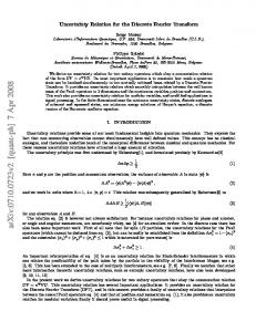
We adopted a sample size of 120

observations corresponding, for example, to 30 years of quarterly data and adopted the passband of (6,1.5) years or equivalently (24,6) quarters. In terms of frequency (or inverted period), the passband is given by (1/24,1/6) = (0.042,0.167). The frequency response is depicted in Figure 1 and is derived by applying (2) to the unit impulse series and applying the ideal frequency response at the Fourier frequency ordinates (defined by the ‘dot’ points in Figure 1). This operation is implemented in the frequency domain. It is evident from inspection of Figure 1 that the ideal frequency response is synthesized at the Fourier frequency ordinates. It should be noted that while the curve in Figure 1 appears to be continuous, the frequency response function is only strictly defined at the discrete Fourier frequency ordinates themselves. As such, it is not a continuous function of frequency. Thus, while the ‘ripples’ associated with the Gibbs Effect have not disappeared in the context of the discrete-time Fourier Transform representation, these ‘ripples’ are not observable when using the DFT. Specifically, the ‘ripple effect’ associated with the discrete-time Fourier Transform representation of the Gibbs phenomena would arise in the continuous frequency domain at ‘frequency points’ in the continuum that lie between the discrete set of Fourier frequency ordinates associated

12 with the DFT representation.

However, this continuum of frequency

points lying between the discrete Fourier frequency ordinates is not observable or identifiable when using the DFT – the so-called ‘omission’ aspect associated with this outcome that was mentioned above.

This

result is unavoidable given the finite length of the data confronting macroeconomists. However, at each observable or identifiable Fourier frequency ordinate associated with the DFT, it is possible to synthesize an ideal frequency response as shown in Figure 1, which, in aggregate, can be strictly defined across the discrete set of Fourier frequency ordinates. Figure 1 about here.

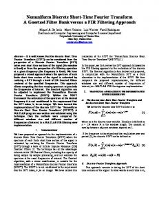
The application of the inverse DFT (3) to the discrete ideal frequency response outlined in Figure 1 is documented in Figure 2. This figure contains a plot of the resulting Dirichlet function which is symmetrical about N/2, i.e. data point 60 in Figure 2. Once again, this function is strictly defined only at the discrete data points represented by the ‘dots’ in Figure 2. It is not a continuous function in time. Moreover, because the Dirichlet function is the inverse DFT of (discrete) ideal frequency response function displayed in Figure 1, it can be viewed as depicting a discrete finite symmetrical set of (time-domain) filter coefficients. Furthermore, because of the finite extent of this set of filter coefficients, the inverse DFT has naturally and automatically imposed a truncation process on the sequence of filter coefficients.

13 Figure 2 about here.

The space between adjacent Fourier frequency ordinates is determined by the fundamental frequency f 1 =

1 , which is the upper limit for N

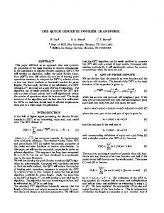
resolving cycles in the finite segment of the time series. The larger is the sample size N, the finer will be the grid resolution of Fourier frequency ordinates and the smaller will be the difference between neighbouring Fourier frequency ordinates themselves. This can be seen in Figure 3 which displays the frequency response function for a unit impulse sequence of 240 observations. It is apparent from inspection of Figures 3 and 1 that the grid ‘mesh’ of the frequency response function outlined in Figure 3 is of a much finer resolution when compared with that displayed in Figure 1. Note further that the discrete ideal frequency response continues to be synthesized in Figure 3 at a finer grid resolution – each Fourier frequency in the passband continues to display a value of unity while each Fourier frequency outside the passband continues to have a value of zero. Moreover, the frequency response function continues to be strictly defined only at the Fourier frequency ordinates themselves.

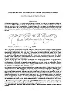
Figure 3 about here. The inverse DFT (or Dirichlet function) of the ideal frequency response displayed in Figure 3 is outlined in Figure 4. Recall that this function is symmetrical about N/2, i.e. data point 120 in Figure 4 and is only strictly defined at the discrete points represented by the ‘dots’ points in

14 Figure 4. It also represents a set of finite symmetrical discrete (timedomain) filter coefficients. It is apparent from inspections of Figures 4 and 2 that fluctuations in the Dirichlet function have become smoother (i.e. smaller in absolute value) as the sample size N has been increased.

Figure 4 about here. From the perspective of understanding and combating the effects of the Gibbs phenomena, the key determinant of this effect has been demonstrated to be the finite truncation associated with the imposition of the ideal frequency response. The key aspect of the truncation process is the resulting discontinuity that is imposed by the ‘0-1’ step function that is imposed at the ‘stopband-passband’ transition [see Papoulis (1962, pp.30-31), Kufner and Kadlec (1971, pp. 225-228), Bracewell (1978, 209-211), Priestley (1981, p.561)]. In fact, the application of the discrete-time Fourier Transform at the point of discontinuity directly produces the ripple phenomenon associated with the Gibbs Effect. One way to reduce any impact of the Gibbs Effect is to smooth the transition between the stopband and bandpass cutoffs, thus reducing the size of the point of discontinuity alluded to above. A proposal to this effect has been recently advocated in Iacobucci-Noullez (2004, 2005) who proposed the use of a convolved windowed Bandpass DFT Filter Algorithm. This algorithm involves smoothing the ‘0-1’ transition at the stopband-passband cutoffs by using a taper that is linked to specific

15 spectral windows. In this article, we use the ‘Hamming’ spectral window recommended in Iacobucci and Noullez (2004, p.6).

This involves

applying the following smoothing scheme

Vx ( k ) = ( 0.23* H k −1 + 0.54* H k + 0.23* H k +1 ) * Ax ( k ) .

(6)

In the above equation, Ax ( k ) is derived from (2) – that is, by applying the DFT to the input data series x ( tn ) and H k is based upon the discrete ideal

frequency

response

H ( f k ) = 1 for k1 ≤ k ≤ k2 , -k2 ≤ −k ≤ −k1 ,

otherwise zero. As such, the smoothing occurs in the frequency domain. The Filtering operation outlined in (4) can then be represented as

yɶ ( tn ) =

1  k2 kn  N − k1 kn     exp 2 V f i π ( ) ∑ k   + ∑ V ( f k ) exp  i 2π   , N  k = k1 N  k = N − k2 N   

(7)

where V ( f k ) is equal to V x (k ) in (6) and where f k =

k is the Fourier N

frequency corresponding to frequency index k. The frequency response function for the Iacobucci-Noullez filter is documented in Figure 5. In this figure, the frequency response associated with the conventional DFT algorithm is included as a point of reference (for sample size of 120 observations).

The main point of

difference is that the Iacobucci-Noullez filter has a smoother (tapered) transition from the stopband to passband region involving the following response pattern (from the low frequency end) of {0.0,0.23,0.7,1.0,1.0} while the conventional DFT filter has transition response pattern of

16 {0.0,0.0,1.0,1.0,1.0}. It is evident from the above patterns that the ‘0-1’ transition has been smoothed by invoking smaller incremental changes – that is from 0-0.23, 0.23-0.7 and 0.7-1, thereby reducing the size of the conventional ‘0-1’ discontinuity at the ‘stopband-passband’ transition to a series of smaller incremental steps. However, this smoothing process allows for the possibility of increased leakage from components in the stopband to the bandpass filtered data. In particular, components in the stopband region that are very close to the ‘stopband-passband’ transition could be incorrectly passed to the bandpass filtered data. For example, a weight of 0.23 would be assigned to the low frequency component falling immediately before the passband transition and this component would be included in the derivation of the bandpass filtered data series. Therefore if this low frequency component has a non-zero value, then some contribution from this component would be passed to the bandpass filtered data series even though this component clearly falls in the stopband, thus producing some ‘contamination’ of the filtered data series obtained from the Iacobucci-Noullez filter.

Figure 5 about here. In Figure 6, we display the Dirichlet function (inverse DFT) of the frequency response functions outlined in Figure 5.

The main effect of

tapering associated with the Iacobucci-Noullez filter is to dampen out the fluctuations in the Dirichlet function when compared with that associated with conventional DFT.

As such, the set of discrete filter

17 coefficients associated with the Iacobucci-Noullez filter are closer to zero in absolute value for a large band of data points (i.e. lagged filter coefficient values) displayed in Figure 6. It should also be recognized that the theory underpinning Fourier analysis is based on the concept of stationary time series. Therefore, it is crucial to establish what mechanism (deterministic or stochastic) is generating the trend and propose actions to remove the trend prior to performing any DFT based filtering operations. Unless stated otherwise, we assume that the data has been rendered stationary. However, if the data series has not been de-trended or has been inappropriately de-trended, then either the prominent low frequency components or other spurious structure (generated from inappropriately applied de-trending methods) will be capable of generating leakage effects capable of distorting the bandpass filtered data series obtained from the filters. Tapering, in this case, however, is not the appropriate remedial action.

The correct remedy, instead, is to de-trend the data series

correctly, possibly utilizing some theoretical model explaining the longrun behaviour that is encapsulated in the trend properties of the underlying data series.

3

SIMULATION MODEL

We wrote a FORTRAN 95 program to conduct the reported simulations. In general terms, the artificial data model can be viewed as a periodic

18 process that can be deterministic or embedded in stationary Gaussian noise. The ‘complete’ periodicity is defined as the sum of two orthogonal periodicities. The first is a low frequency periodicity that is deliberately designed to fall outside the passband of interest, while the second periodicity is deliberately designed to fall within the passband. Unless stated otherwise, we adopt the same parameter settings that were outlined in relation to Figure 1 in the previous section. Formally, we define the low frequency periodicity as

xl (t ) = amp1 * sin (2πf 1 * (t + 10)) ,

(8)

and the ‘bandpass’ periodicity is defined as

xb (t ) = amp 2 * cos(2πf 2 * (t − 4 )) ,

(9)

where amp1 and amp2 are amplitude parameters while f1 and f 2 are frequency parameters. In all simulations reported in this article, we adopt the following parameter settings for the ' amp' variables: amp1 = 5.0 and amp 2 = 1.0 . The complete periodicity can be represented by

x(t ) = xl (t ) + xb (t ) + ε (t ) ,

(10)

where ε (t ) is a stationary random process. In this article ε (t ) can take the following forms:

ε (t ) = 0

(11)a

where xl ( t ) , xb ( t ) and x ( t ) are purely deterministic periodic processes; or

19

ε (t ) = u (t ) ,

(11)b

where u (t ) (and ε (t ) ) is a stationary Gaussian noise process, x ( t ) is a stochastic periodic process while both xl ( t ) and xb ( t ) are deterministic periodic processes.

Both plots and detailed discussion of these data

series can be found in Hinich, Foster and Wild (2007). In relation to that discussion, we wish to stress the following points. First, the true low frequency periodicity given by f 1 = 0.025 is perfectly synchronized with the Fourier frequency ordinate 0.025 in the low frequency region of the stopband. Second, the main difference in parameter settings adopted in (9) for the true ‘bandpass’ periodicity reflects our desire to examine the implications on filtering of two specific circumstances.

The first corresponds to the situation when the true

‘bandpass’ periodicity is perfectly synchronized with a Fourier frequency ordinate in the passband. In this case, the f 2 parameter is set to 0.0667. The second circumstance is when the true ‘bandpass’ periodicity lies between two adjacent Fourier frequency ordinates in the passband. This ‘unsynchronized’ case corresponds to a parameter setting for

f 2 of

0.0625. The data generated by deterministic model [(10)-(11)a] and stochastic model [(10)-(11)b] represents the ‘input’ data series x(t n ) that the time to frequency DFT in (2) is applied to. The specific data series generated by

20 (9) for various f 2 parameter settings are the respective targets of the bandpass filtering operations of both DFT filters.

4

RESULTS ASSOCIATED WITH THE DETERMINSTIC PERIODIC

MODEL (10)-(11)A - EQ (9): F2 = 0.0667 AND EQ (9): F2 = 0.0625 In this section, we investigate the ability of the various bandpass filters to extract the deterministic ‘bandpass’ cycle which is (and is not) perfectly synchronized with a Fourier frequency ordinate in the passband. bandpass

The basis of the testing procedure is to apply the various filters

to

the

artificial

data

series

generated

by

the

deterministic periodic model [[10)-(11)a]. Our objective is to examine the comparative performance of both DFT filters in tracking the target data series generated by (9). Figure 7 contains a plot of the results from application of both DFT filter algorithms to the synchronized deterministic model [(10)-(11)a] with

f 2 = 0.0667 in (9). In this figure, the artificial data series associated with the true ‘bandpass’ periodicity determined by (9) and the bandpass filtered data series from both DFT filters are displayed together.

It is

evident from inspection of this figure that both filters produce data series that perfectly track the true target ‘bandpass’ periodicity – the ‘actual’ data series displayed in Figure 7. Therefore, both filter algorithms successfully

and

completely

extracted

the

deterministic

corresponding to the synchronized ‘bandpass’ periodicity.

cycle

21

Figure 7 about here. In order to confirm that the DFT filter operations have ignored the low frequency periodicity contained in (10) [subsequently generated by (8)], we make use of the periodogram of the bandpass filtered data series. The periodogram of the data series is calculated as the squared modulus of the complex variable Ax (k ) determined from (2) for each Fourier frequency k divided by the number of sample points N . If the low frequency cycle has been removed from the filtered data series, then there should be no ‘power’ (i.e. no non-zero value) evident at the low frequency ordinate (0.025) in the periodogram of the filtered series. The periodograms of both DFT filtered data series are displayed in Figure 8. Examination of Figure 8 indicates that the low frequency component has been successfully expunged from the filtered data series of both bandpass filters – there is no power corresponding to Fourier frequency ordinate 0.025. In both cases, the only power corresponds to the spike at

Fourier

frequency

ordinate

0.0667

reflecting

the

perfect

synchronization with the true ‘bandpass’ periodicity generated by (9). The exact correspondence between the two filtered data series can be seen from the fact that both filters display the exact same power at Fourier frequency ordinate 0.0667 in Figure 8.

Figure 8 about here.

22 We also investigated the ability of the two DFT filters to extract the true deterministic ’bandpass’ cycle which is not synchronized with any Fourier frequency ordinate in the passband.

In this case, the true

‘bandpass’ periodicity using (9) corresponds to the ‘unsynchronized’ case with associated value for parameter f 2 of 0.0625 which was designed to fall half way between the adjacent Fourier frequency ordinates 0.0583 and 0.0667. In Hinich, Foster and Wild (2007), it was demonstrated that in this case, the true periodicity would be ‘smeared’ or ‘spread’ between the adjacent Fourier frequency ordinates that border the true periodicity. Figure 9 contains a plot of the periodograms of the filtered data obtained from application of the DFT filters to the unsynchronized data series.

The first thing to note from inspection of Figure 9 is that the

spike associated with the synchronized case outlined in Figure 8 at frequency 0.0667 has disappeared.

Instead, the true periodicity has

been spread over the neighbouring frequency ordinates 0.0583 and 0.0667. Moreover, there is also some power spread to other adjacent Fourier frequency ordinates in the passband region, although at a diminishing rate. It is also apparent from inspection of Figure 9 that the pattern of dispersion of the ‘unsynchronized’ true bandpass periodicity about neighbouring Fourier frequency ordinates is both qualitatively and quantitatively similar for both DFT filters. The tapering associated with the Iacobucci-Noullez filter does not seem to affect the dispersion pattern.

23

Figure 9 about here. The other major feature is that the low frequency component has been successfully removed from the bandpass filtered data series – there is no power corresponding to Fourier frequency ordinate 0.025. In fact, there is no power discernible outside of the passband. The bandpass filtered data series obtained from application of both DFT filters has successfully expunged all ‘stopband’ components from the filtered data series. A key question relates to the nature of possible distortions that the observed smearing of the true ‘bandpass’ periodicity by the DFT filters may exert on the ability of the filtered data series to replicate the true ‘bandpass’ periodicity.

The nature of the distortions can be discerned

from Figure 10 which contains plots of the DFT filtered data series against the unsynchronized true ‘bandpass’ periodicity.

Figure 10 about here. It is apparent from inspection of Figure 10 that, apart from some noticeable albeit minor deviations at both endpoints, the filtered data series seems to track the true ‘bandpass’ periodicity remarkably well. Upon closer inspection, there is some slight differences between the three series – the ‘dot points’ for these series do not coincide exactly although they are typically quite close to each other except at the endpoints. Figure 11 contains a plot of the two bandpass filtered data series. It is evident from inspection of this figure that the two filtered data series

24 track each other extremely closely. Therefore, the deviations apparent in Figure 10 principally reflect deviations between the true ‘bandpass’ periodicity and both filtered data series more generally, particularly at the endpoints.

Figure 11 about here. To summarize, the most striking result to emerge is the marked ability of both DFT filters to extract the true target ‘bandpass’ periodicities. Extraction was exact in the case of the ‘synchronized’ bandpass periodicity. In the case of the ‘unsynchronized’ bandpass periodicity, the DFT filters continue to come close to extracting the true target periodicity, provided that we ignore some minor distortions at the endpoints of the filtered data series. These distortions have been introduced because of the smearing of the true periodicity associated with the filtering operation, but for the most part (i.e. away from the endpoints), these distortions appear to be very small in magnitude. Furthermore, the results for both DFT filters almost coincide exactly – the actual nature of the observed deviations more accurately and generally reflect deviation between the true target ‘bandpass’ periodicity and both filtered data series. Finally, the tapering operation implied in (6) seems to have no noticeable effect when compared with the results produced by the conventional DFT filter. Thus, the possibility of adverse affects attributable to the Gibbs phenomena did not appear to emerge.

25 The results cited in the current section are obtained for an underlying deterministic periodic data series. We now investigate whether these broad conclusions continue to hold when the deterministic ‘bandpass’ periodicity is embedded in a stationary Gaussian noise process.

5

RESULTS ASSOCIATED WITH THE STOCHASTIC STATIONARY

GAUSSIAN PERIODIC MODEL (10)-(11)B In this section, we investigate the ability of the DFT filters to extract the ‘bandpass’ periodicity when the deterministic periodicities (8)-(9) are embedded in a stationary Gaussian noise process according to the stochastic model (10)–(11)b. The basis of the testing procedure employed in this section will be to apply the various bandpass filters to the artificial data series generated by (10) and assess the extent to which the properties of the deterministic ‘bandpass’ periodic data generated by (9) appear to be reflected in the respective filtered data series. Examination of filter performance will be based on standard summary measures of goodness of fit in order to ascertain how ‘close’ the filtered series approximates the target ‘bandpass’ periodicities. However, an important additional consideration will center upon whether the filtering operations have generated data series in which the low frequency periodicity associated with (8) has been successfully expunged from the filtered data series. In order to confirm that both DFT filter operations have ignored the low frequency periodicity generated by (10), we inspect

26 the periodograms of both filtered data series which are documented in Figures 12 and 13 respectively.

Figure 12 about here. Examination of Figure 12 relating to the synchronized model indicates that the low frequency component has been successfully expunged from both filtered data series – there is no power corresponding to Fourier frequency ordinate 0.025. For this particular case and both filters, the main power in the filtered series occurs at Fourier frequency ordinate 0.0667 and 0.1583 respectively.

The first ordinate is the Fourier

frequency ordinate that is synchronized with the f 2 value of 0.0667 used in (9).

Figure 13 displays the results for the unsynchronized case

corresponding to parameter setting of

f 2 = 0.0625 in (9).

In this

particular case, the ‘true’ periodicity of 0.0625 has been spread over the neighbouring frequency ordinates 0.0583 and 0.0667. identified

at

Fourier

frequency

0.1583

is

also

The power

evident

in

the

unsynchronized case as well.

Figure 13 about here. It is also apparent from inspection of Figures 12 and 13 that the pattern of

dispersion

for

both

the

‘synchronized’

and

‘unsynchronized’

periodicities about neighbouring Fourier frequency ordinates is both qualitatively and quantitatively similar for both DFT filters.

Thus, the

observation made in the previous section about the tapering associated

27 with the Iacobucci-Noullez filter appearing not to affect the observed periodiogram dispersion patterns continue to hold. In Hinich, Foster and Wild (2007), it was argued that the observed power at the second Fourier frequency ordinate 0.1583 was most probably an artifact of the noise process which when combined with the deterministic periodicity produced a harmonic effect. Whatever the cause, these two frequencies are clearly in the passband range. It should also be noted that for both cases, the noise process more generally produced small amounts of power at all Fourier frequencies in the passband

although

this

outcome

was

more

noticeable

in

the

‘unsynchronized’ case represented in Figure 13. This contrasts with the lack of ‘power’ outside of the passband, thus clearly encapsulating the desired ideal frequency response in the stopband region. In order to get some idea of how closely the DFT filtered data series track each other, comparative plots of the filtered data series are displayed in Figures 14 and 15 for the synchronized and unsynchronized models respectively. It is apparent from inspection of both figures that the two DFT filters produce data series that track each other very closely.

Figure 14 about here. Figure 15 about here. Because of the apparent amplitude and phase variation in the filtered data generated by the two filters considered in the article when compared

28 to deterministic ‘target’ periodicities generated by (9), we must resort to conventional

goodness-of–fit

measures

to

get

some

idea

comparative performance of the two different DFT filters.

of

the

In this

approach, the target periodicity is viewed heuristically as the dependent variable in a regression model while the filtered data series from the various filters is treated as the predicted value from the regression model itself. In this context, the filter that produces the best fit according to the standard goodness-of-fit criteria would be judged the best. The goodness-of-fit results for the synchronized case are outlined in Table 1. It should be noted that the first two rows of the Table relating to the mean and standard deviation are applied to a calculated residual series, determined as the difference between the filtered data series and the respective true ‘bandpass’ periodicity.

All the other statistics are

calculated directly from the two respective data series. 2 It is apparent from inspection of the second and third columns of Table 1 that the Iacobucci-Noullez filter has marginally better ‘goodness-of-fit’ statistics – the tapering of the ‘stopband-passband’ edges seems to improve the fit marginally in the synchronized case.

2 All statistics are calculated using the following worksheet functions in Excel – ‘AVERAGE’, ‘STDEV’, ‘CORREL’, ‘RSQ’ and ‘STEYX’.

29 The results for the unsynchronized data are listed in Table 2.

It is

evident from inspection of Table 2 that the conclusions made about the DFT filters immediately above should now be reversed - the conventional DFT filter appears to be marginally ‘superior’ to the Iacobucci-Noullez filter on all statistical counts. Overall, the results cited in Tables 1 and 2 and displayed in Figures 12 - 15 continue to support the broad substantive conclusions made in the previous section in relation to the two DFT filters. In particular, the role of the tapering operation in (6) seems to produce no noticeable difference in simulation results, thus calling into question, the pervasiveness of the Gibbs effect associated with the ‘0-1’ ‘stopband-passband’ transition implied in conventional DFT filter algorithm.

6

CONCLUSIONS

In this article, we examined the nature and role of the effects that could potentially be exerted upon business cycle extraction attempts from the Gibbs Effect. Our objective was to examine this issue from the perspective

of

the

actual

environment

that

confronts

applied

macroeconomists – namely, situations involving a single realization of a small to moderate sized sample of discrete-time macroeconomic data. We argued that the nature of the data confronting macroeconomists meant that the appropriate Fourier Transform concept was the Discrete

30 Fourier Transform. In contrast, theoretical representations of the Gibbs Effect are derived from the discrete-time Fourier Transform. However, we argued that these theoretical results could be misleading in practice when using the DFT. Our general conclusion was that none of the problems associated with the Gibbs Effect will affect the filtering of a finite length data series using the DFT although this result carried a caveat of ‘omission’. Essentially, the Gibbs Effect was not observable or identifiable at the frequency ordinates associated with the DFT. More particularly, we showed that the ideal frequency response could be synthesized at the discrete set of Fourier frequency ordinates – the only frequency ordinates identifiable using the DFT. The ‘ripple effect’ associated with the Gibbs phenomena could be interpreted as arising in the ‘continuous’ frequency domain at points in the continuum that lie between the discrete set of Fourier frequency ordinates associated with the DFT – these frequency points, however, were not observable or identifiable using the DFT. It was shown that one way to reduce any impact of the Gibbs effect would be to smooth the transition between the stopband and bandpass cutoffs. Recently Iacobucci-Noullez (2004, 2005) proposed this action and advocated the use of a convolved windowed DFT Filter Algorithm. In order to gauge the possible importance of the Gibbs Effect, we assessed

31 the comparative performance of conventional DFT filter with the filter proposed by Iacobucci-Noullez that utilized the Hamming window. In order to investigate the cycle extraction properties of the filters more generally, we conducted simulations involving artificial data generated from a model of a periodic process that could be potentially deterministic or embedded in stationary Gaussian noise. The ‘complete’ periodicity was defined as the sum of two orthogonal periodicities. The first was a low frequency periodicity that was deliberately designed to fall outside the passband of interest, while the second periodicity was deliberately designed to fall within the passband. We also distinguished between the cases where the true ‘bandpass’ periodicity was synchronized with a Fourier frequency ordinate in the passband. It was established that under this particular circumstance, the DFT filters would work optimally.

The second case was when the

true periodicity was not synchronized with a Fourier frequency ordinate. In this case, it was demonstrated that the true periodicity would be smeared between the Fourier frequency ordinates bordering it which was capable of producing distortions between the true periodicity and the filtered data series especially at the start and end points of the filtered data series. However, apart from the endpoints, the distortions appeared to be very small in magnitude and were both qualitatively and quantitatively the same for both filters considered and also across all simulation models utilized.

32 More generally, the qualitative and quantitative similarity of the results obtained for both DFT filters across the range of simulations called into question the practical implications of the Gibbs Effect.

The tapering

associated with the Iacobucci-Noullez filter produced no qualitative or quantitative differences from the results obtained from the conventional DFT filter.

If the Gibbs Effect had a significant practical role to play,

then we would expect the tapering associated with the Iacobucci-Noullez filter to generate results that were different from those associated with the conventional DFT filter.

33

Table 1.

Summary Statistics of Goodness of Fit of Synchronized

Deterministic Target Bandpass Periodicity [Eq (10)-(11)a: f 2 = 0.0667 ] and Filtered Data Obtained From Various DFT Bandpass Filters DFT

IAC_Ham

Mean

0.0000

0.0000

Std Dev

0.6182

0.6175

Correlation

0.7276

0.7280

R Squared

0.5294

0.5300

Std Error

0.4891

0.4889

Table 2. Summary Statistics of Goodness of Fit of Unsynchronized Deterministic Target Bandpass Periodicity [Eq (10)-(11)b: f 2 = 0.0625 ] and Filtered Data Obtained From Various DFT Bandpass Filters DFT

IAC_Ham

Mean

-0.0419

-0.0419

Std Dev

0.6346

0.6360

Correlation

0.6496

0.6465

R Squared

0.4220

0.4179

Std Error

0.5412

0.5431

34

REFERENCES Baxter, M. and R. G. King (1999) Measuring business cycles: approximate band-pass filters for economic time series. The Review of Economics and Statistics 81, 575-593. Bracewell, R. N. (1978) The Fourier Transform and its Applications. Second Edition. New York: McGraw-Hill. Hinich, M. J., Foster, J. and P. Wild (2007) An Investigation of the Cycle Extraction Properties of Several Bandpass Filters used to Identify Business Cycles. School of Economics, University of Queensland, February 2007, Mimeo. Hodrick, R. J. and E. C. Prescott (1997) Postwar U.S. business cycles: an empirical investigation. Journal of Money, Credit, and Banking 29, 1-16. Iacobucci, A. and A. Noullez (2004) A frequency selective filter for shortlength time series. OFCE Working paper N 2004-5. (Available at:http://repec.org/sce2004/up.4113.1077726997.pdf). Iacobucci, A. and A. Noullez (2005) A frequency selective filter for shortlength time series. Computational Economics 25, 75-102. Kufner, A. and J. Kadlec. (1971) Fourier Series. Prague: Academia. Papoulis, A. (1962) The Fourier Integral and Its Applications. New York: McGraw-Hall. Priestley, M. B. (1981) Special Analysis and Time Series. London: Academic Press.

35

Figure 1. Plot of Frequency Response of Bandpass Filter for Unit Impulse - Sample Size = 120, Passband = (0.042,0.167) 1.2000

1.0000

Value

0.8000

0.6000

freq resp

0.4000

0.2000

0. 00 0 0. 0 01 6 0. 7 03 3 0. 3 05 0 0. 0 06 6 0. 7 08 3 0. 3 10 0 0. 0 11 6 0. 7 13 3 0. 3 15 0 0. 0 16 6 0. 7 18 3 0. 3 20 0 0. 0 21 6 0. 7 23 3 0. 3 25 0 0. 0 26 6 0. 7 28 3 0. 3 30 0 0. 0 31 6 0. 7 33 3 0. 3 35 0 0. 0 36 6 0. 7 38 3 0. 3 40 0 0. 0 41 6 0. 7 43 3 0. 3 45 0 0. 0 46 6 0. 7 48 3 0. 3 50 00

0.0000

Frequency

Figure 2. Plot of Inverse DFT (Dirichlet Function) of Bandpass Filter for Unit Impulse - Sample Size=120, Passband = (0.042,0.167) 0.3000 0.2500 0.2000 0.1500

0.0500

dirichlet

-0.0500 -0.1000 -0.1500 -0.2000 Data Points

3

9

7 11

11

10

1

5 10

97

10

93

89

85

81

77

73

69

65

61

57

53

49

45

41

37

33

29

25

21

17

9

13

5

0.0000

1

Values

0.1000

36

Figure 3. Plot of Frequency Response of Bandpass Filter for Unit Impulse - Sample Size = 240, Passband = (0.042,0.167) 1.2000

1.0000

Value

0.8000

0.6000

freq resp

0.4000

0.2000

0. 00 0 0. 0 01 6 0. 7 03 3 0. 3 05 0 0. 0 06 67 0. 08 3 0. 3 10 0 0. 0 11 6 0. 7 13 3 0. 3 15 0 0. 0 16 6 0. 7 18 3 0. 3 20 0 0. 0 21 6 0. 7 23 3 0. 3 25 0 0. 0 26 6 0. 7 28 3 0. 3 30 0 0. 0 31 6 0. 7 33 33 0. 35 0 0. 0 36 6 0. 7 38 3 0. 3 40 0 0. 0 41 6 0. 7 43 3 0. 3 45 0 0. 0 46 6 0. 7 48 3 0. 3 50 00

0.0000

Frequency

Figure 4. Plot of Inverse DFT (Dirichlet Function) of Bandpass Filter for Unit Impulse - Sample Size=240, Passband = (0.042,0.167) 0.3000 0.2500 0.2000 0.1500

0.0500

dirichlet

-0.0500 -0.1000 -0.1500 -0.2000 Data Points

239

232

225

218

211

204

197

190

183

176

169

162

155

148

141

134

127

120

113

99

106

92

85

78

71

64

57

50

43

36

29

22

8

15

0.0000

1

Values

0.1000

37

Figure 5. Plot of Frequency Response of Selected DFT Bandpassed Filters for Unit Impulse - Sample Size = 120, Passband = (0.042,0.167) 1.2000

1.0000

Value

0.8000

Conv DFT Iac_Ham

0.6000

0.4000

0.2000

0. 00 0 0. 0 01 6 0. 7 03 3 0. 3 05 0 0. 0 06 6 0. 7 08 3 0. 3 10 0 0. 0 11 6 0. 7 13 3 0. 3 15 0 0. 0 16 6 0. 7 18 3 0. 3 20 0 0. 0 21 6 0. 7 23 3 0. 3 25 0 0. 0 26 6 0. 7 28 3 0. 3 30 0 0. 0 31 6 0. 7 33 0. 33 35 0 0. 0 36 6 0. 7 38 3 0. 3 40 0 0. 0 41 6 0. 7 43 3 0. 3 45 0. 00 46 6 0. 7 48 3 0. 3 50 00

0.0000

Frequency

Figure 6. Plot of Inverse DFT (Dirichlet Function) of Selected DFT Bandpass Filters for Unit Impulse Sample Size=120, Passband = (0.042,0.167) 0.3000 0.2500 0.2000 0.1500

Conv DFT Iac_Ham

0.0500

-0.0500 -0.1000 -0.1500 -0.2000 Data Points

97 10 1 10 5 10 9 11 3 11 7

93

89

85

81

77

73

69

65

61

57

53

49

45

41

37

33

29

25

21

17

9 13

5

0.0000

1

Values

0.1000

38

Figure 7. Comparison of DFT Filtered Data Series From Deterministic Model [Eq (10) and Eq (11)a] and Actual (Target) Synchronized Bandpass Periodicity Data [Eq (9): f2 = 0.0667] - Sample Size = 120 1.5000

1.0000

3

7 11

11

5

1

9 10

10

97

10

93

89

85

81

77

73

69

65

61

57

53

49

45

41

37

33

29

25

21

17

9

13

5

0.0000

1

Values

0.5000

DFT filter actual IAC_Ham

-0.5000

-1.0000

-1.5000 Data Points

Figure 8. Plots of Periodograms of DFT Filtered Data Series Derived From Synchronized Deterministic Model [Eq (10) - Eq (11)a, Eq(9): f2=0.0667]: DFT and IAC_Hamming Filters - Sample Size=120, Passband = (0.042,0.167) 35.0000

30.0000

25.0000

Value

20.0000 DFT IAC_Ham 15.0000

10.0000

5.0000

0. 00 0. 00 01 0. 67 03 3 0. 3 05 0. 00 06 6 0. 7 08 0. 33 10 0. 00 11 6 0. 7 13 3 0. 3 15 0 0. 0 16 6 0. 7 18 0. 33 20 0 0. 0 21 6 0. 7 23 3 0. 3 25 0. 00 26 6 0. 7 28 3 0. 3 30 0 0. 0 31 0. 67 33 0. 33 35 0 0. 0 36 6 0. 7 38 33 0. 40 0. 00 41 0. 67 43 3 0. 3 45 0. 00 46 6 0. 7 48 0. 33 50 00

0.0000

Frequency

39

Figure 9. Plots of Periodograms of DFT Filtered Data Series Derived From Unsynchronized Deterministic Model [Eq (10)- Eq (11)a, Eq(9): f2=0.0625]: DFT and IAC_Hamming Filters - Sample Size=120, Passband = (0.042,0.167) 14.0000

12.0000

10.0000

Value

8.0000 DFT IAC_Ham 6.0000

4.0000

2.0000

0. 00 0. 00 01 0. 67 03 3 0. 3 05 0. 00 06 6 0. 7 08 0. 33 10 0. 00 11 6 0. 7 13 3 0. 3 15 0 0. 0 16 6 0. 7 18 0. 33 20 0 0. 0 21 6 0. 7 23 3 0. 3 25 0. 00 26 6 0. 7 28 3 0. 3 30 0 0. 0 31 0. 67 33 0. 33 35 0 0. 0 36 6 0. 7 38 33 0. 40 0. 00 41 0. 67 43 3 0. 3 45 0. 00 46 6 0. 7 48 0. 33 50 00

0.0000

Frequency

Figure 10. Comparison of DFT Filtered Data Series From Deterministic Model [Eq (10) - Eq (11)a] and Actual (Target) Unsynchronized Bandpass Periodicity Data [Eq (9): f2=0.0625] - Sample Size = 120 1.5000

1.0000

-0.5000

-1.0000

-1.5000 Data Points

97 10 1 10 5 10 9 11 3 11 7

93

89

85

81

77

73

69

65

61

57

53

49

45

41

37

33

29

25

21

17

9

13

5

0.0000

1

Values

0.5000

DFT filter actual IAC_Ham

40

Figure 11. Comparison of DFT Filtered Data Series From Deterministic Model [Eq (10) - Eq (11)a] for Unsynchronized Periodicity Data [Eq (9): f2=0.0625] - Sample Size = 120 1.5000

1.0000

DFT filter IAC_Ham

3

9

5

1

7 11

11

10

10

97

10

93

89

85

81

77

73

69

65

61

57

53

49

45

41

37

33

29

25

21

17

9

13

5

0.0000

1

Values

0.5000

-0.5000

-1.0000

-1.5000 Data Points

Figure 12. Plot of Periodograms of DFT Filtered Data Series Derived From Synchronized Stochastic "I(0)" Model [Eq (10) Eq (11)b, Eq(9): f2 = 0.0667]: DFT and IAC_Hamming Filters - Sample Size = 120, Passband = (0.042,0.167) 30.0000

25.0000

DFT

15.0000

IAC_Ham

10.0000

5.0000

0.0000 0. 00 00 0. 01 67 0. 03 33 0. 05 00 0. 06 67 0. 08 33 0. 10 00 0. 11 67 0. 13 33 0. 15 00 0. 16 67 0. 18 33 0. 20 00 0. 21 67 0. 23 33 0. 25 00 0. 26 67 0. 28 33 0. 30 00 0. 31 67 0. 33 33 0. 35 00 0. 36 67 0. 38 33 0. 40 00 0. 41 67 0. 43 33 0. 45 00 0. 46 67 0. 48 33 0. 50 00

Value

20.0000

Frequency

41

Figure 13. Plot of Periodograms of DFT Filtered Data Series for Unsynchronized Stochastic "I(0)" Model [Eq (10)- Eq (11)b, Eq(9): f2=0.0625]: DFT and IAC_Hamming Filters - Sample Size = 120, Passband = (0.042,0.167)

10.0000

9.0000

8.0000

7.0000

Value

6.0000 DFT

5.0000

IAC_Ham

4.0000

3.0000

2.0000

1.0000

0. 00 00 0. 01 67 0. 03 33 0. 05 00 0. 06 67 0. 08 33 0. 10 00 0. 11 67 0. 13 33 0. 15 00 0. 16 67 0. 18 33 0. 20 00 0. 21 67 0. 23 33 0. 25 00 0. 26 67 0. 28 33 0. 30 00 0. 31 67 0. 33 33 0. 35 00 0. 36 67 0. 38 33 0. 40 00 0. 41 67 0. 43 33 0. 45 00 0. 46 67 0. 48 33 0. 50 00

0.0000

Frequency

Figure 14. Comparison of DFT Filtered Data Series For Synchronized Stochastic "I(0)" Model [Eq (10)-(11)b, Eq(9):f2 = 0.0667]: DFT and IAC_Hamming Filters - Sample Size=120

2.5000

2.0000

1.5000

1.0000

DFT

0.0000

-0.5000

-1.0000

-1.5000

-2.0000

-2.5000 Data Points

94 97 10 0 10 3 10 6 10 9 11 2 11 5 11 8

88 91

82 85

76 79

70 73

64 67

58 61

52 55

46 49

40 43

34 37

28 31

22 25

16 19

7 10 13

IAC_Ham 4

1

Values

0.5000

42

Figure 15. Comparison of DFT Filtered Data Series From Unsynchronized Stochastic "I(0)" Model [Eq (10)-(11)b, Eq(9): f2 = 0.0625]: DFT and IAC_Hamming Filters - Sample Size=120

2.0000

1.5000

1.0000

DFT

0.0000

-0.5000

-1.0000

-1.5000

-2.0000 Data Points

94 97 10 0 10 3 10 6 10 9 11 2 11 5 11 8

91

88

85

82

79

76

73

70

67

64

61

58

55

52

49

46

43

40

37

34

31

28

25

22

19

16

7 10 13

IAC_ham 4

1

Values

0.5000