FFT techniques follow Shannon's sampling theorem [ref. 2]. This theorem states the basic relationships between the sampling rate of the data and the frequency ...
972006
The Time Variant Discrete Fourier Transform as an Order Tracking Method Jason R. Blough and David L. Brown Structural Dynamics Research Laboratory University of Cincinnati
Håvard Vold Vold Solutions
ABSTRACT Present order tracking methods for solving noise and vibration problems are reviewed, both FFT and resampling based order tracking methods. The time variant discrete Fourier transform (TVDFT) is developed as an alternative order tracking method. This method contains many advantages which the current order tracking methods do not possess. This method has the advantage of being very computationally efficient as well as the ability to minimize leakage errors. The basic TVDFT method may also be extended to a more complex method through the use of an orthogonality compensation matrix (OCM) which can separate closely spaced orders as well as separate the contributions of crossing orders. The basic TVDFT is a combination of the FFT and the re-sampling based methods. This method can be formulated in several different manners, one of which will give results matching the re-sampling based methods very closely. Both analytical and experimental data are used to establish the behavioral characteristics of this new method. INTRODUCTION Traditionally two basic methods have been employed to digitally track orders which result from rotating components in noise and vibration problems. These two basic methods are the FFT based methods and the re-sampling based methods. Recently, a Kalman filtering based method has been introduced to track orders in noise and vibration data. This Kalman filtering based method is not presented in this paper because it is a very different approach to estimating the amplitude and phase of orders. This filtering approach does have many advantages which the two traditional digital methods do not, however, it also has several disadvantages such as the determination of the harmonic confidence factor, and computational load and complexity [ref. 1].
A new method which is presented in this paper is a method which, like the FFT, is based on acquiring constant delta-t spaced time data. This approach however, also makes use of angular position information similar to the re-sampling based methods. The method requires a very accurate tachometer signal, as do all of the order tracking methods. The time variant discrete Fourier transform (TVDFT) method which is presented is based upon a discrete Fourier transform which has a kernel whose frequency is not constant. The frequency of this kernel varies with the frequency of the order of interest. The bandwidth of this technique may be either a constant frequency or a constant order width. Through a post-processing calculation with an orthogonality compensation matrix (OCM), the TVDFT may be extended to separate contributions of closely spaced or crossing orders. This analysis is not possible using either an FFT technique or a re-sampling based technique. The limitations of the orthogonality compensation matrix are discussed and are currently a topic of further research. ORDER TRACKING THEORY FAST FOURIER TRANSFORM BASED ORDER TRACKING - Fast Fourier transform (FFT) based order tracking techniques are probably the most commonly used order tracking methods. These methods are all based upon the FFT and require time domain data sampled with a constant delta-t. These methods require an accurate tachometer signal to allow the computation of the exact frequency which the order of interest possesses at each instant in time. FFT techniques follow Shannon’s sampling theorem [ref. 2]. This theorem states the basic relationships between the sampling rate of the data and the frequency range over which the FFT is performed.
The number of time points and the time spacing between points which are used in the transform determine the delta-f frequency resolution of the FFT. These sampling criteria are presented in Equation 1. ∆f =
1
1
=
N * ∆t
T T = N * ∆t
Fnyquist = Fmax = Fsample =
Fsample
(1)
2
1 ∆t
where: ∆f is the frequency resolution of the resulting frequency spectrum. T is the total sample time which is analyzed. N is the total number of time points over which the transform is performed. ∆t is the time spacing of the time samples. Fsample is the sample frequency of the data. Fnyquist is the Nyquist frequency. Fmax is the maximum frequency which can be analyzed.
The commercially implemented FFT based techniques all require that N be a power of 2 for computational efficiency. These techniques use the transform which is given in Equation 2.
an =
1 N
bn =
1 N
window provides fairly accurate amplitude information as well as fairly good frequency resolution. The second lobe height of -31.47 dB does allow some energy from adjacent frequencies to “leak” into the analyzed frequency bin.
N n =1 N n =1
x(n∆t ) cos(2π f n n∆t ) x(n∆ t ) sin(2πf n n∆t )
(2)
where: fn is the frequency which is being analyzed. an is the Fourier coefficient of the cosine term for fn. bn is the Fourier coefficient of the sine term for fn.
To minimize the effect of leakage on the transform results, a window is applied which forces the analyzed signal to possess a zero slope at both the start and end of the time block. The window which is chosen in this process has a significant effect on the final result. The Hanning or Flattop windows are typically chosen. Unfortunately, all windows which may be applied to the data to reduce leakage have amplitude/frequency resolution tradeoffs. The Hanning window has its first zero at two delta-f’s from the frequency being analyzed and a second lobe height of approximately -31.47 dB. This
The Flattop window has its first zero at four delta-f’s from the frequency being analyzed and a second lobe height of -93.3 dB. This window provides a very accurate amplitude estimate even if the order is not perfectly periodic in the sample window. The disadvantage of this window is the loss of frequency resolution due to its four delta-f frequency width. This large frequency width makes it difficult to separate closely spaced orders, especially at low rpm values where the orders are not well separated in frequency. Once a window is selected, the orders of interest are estimated by performing windowed FFTs on the response signal. Oftentimes, overlap processing is used to give an estimate of the amplitude and phase of the order at more rpm values than would otherwise be possible. The tachometer signal is processed to determine which frequency lines of the FFT correspond to the order of interest. Since the specific order of interest may not fall on a spectral line at every instant in time and its frequency may be changing, multiple spectral lines are summed to give an estimate of the order. If a constant frequency bandwidth estimate is desired, the same number of spectral lines are summed for every rpm. If a constant order bandwidth is desired, a different number of spectral lines is summed for each rpm. More spectral lines are summed at higher rpm values to attain a bandwidth which is proportional to the frequency of the primary order. The rpm assigned to the order estimate is the average rpm over the time period of the FFT. The phase of the order estimate is calculated by performing exactly the same analysis on the tachometer data as is performed on the response data. The phase of the tachometer estimate is then subtracted from the phase of the order estimate to lock the phase of the order estimate to the tachometer signal. Since the FFTs performed on the data are of a constant number of time points at each instant in time, the order estimate is generally more accurate at lower rpm values for lower orders [ref. 3]. The higher rpm/order estimates are less accurate because as the rpm of the machine increases, the frequency of a specific order changes more rapidly. This causes the energy of an order to be spread over more spectral lines in the total sample time of the FFT. This would suggest that a constant order bandwidth should be used to analyze orders using an FFT technique, as this would provide an estimate which is summed over more spectral lines as the rpm increases.
Errors are also introduced because as the frequency of the orders changes rapidly, the amplitude of the orders is also likely to change more rapidly. The order amplitude changes rapidly as the orders approach, excite, and move away from the frequency of a resonance. This phenomena would suggest that as the rpm increases, a shorter time block should be analyzed in a transform. This shorter analysis time is less likely to have a resonance being excited and decaying in the same data block. The analysis of a resonance being excited and decaying significantly in a data block leads to an underestimate in the amplitude of the order. This is due to the fact that the amplitude of the FFT result is the average amplitude of the signal over the total sample time, as shown in Equation 2. This phenomena also suggests that more accurate order estimates will be obtained if the rate of change of the rpm is slow, i.e., a slow sweep rate is suggested for FFT based techniques. Due to the two primary errors discussed here, it can be easily seen that in many instances an FFT approach to order tracking is not as accurate as would be desired. These limitations led to the development of the re-sampling order tracking techniques. RE-SAMPLING BASED ORDER TRACKING Re-sampling based order tracking methods are digital order tracking methods which are much more computationally intensive than the FFT based order tracking methods. The re-sampling based order tracking methods do, however, overcome many of the limitations of the FFT based methods [ref. 4]. Re-sampling based order tracking methods resample constant delta-t sampled data to constant angular intervals [ref. 5]. This process is accomplished through the use of over-sampling, or sampling faster than required by Shannon’s sampling theorem, the constant delta-t sampled data. This over-sampled data is then re-sampled to equal angular intervals using an interpolation algorithm. The times at which the equal angular intervals occur are computed by integrating the tachometer signal. The re-sampled data is now in the angle domain, as opposed to the original time domain. This process can be accomplished in near real time on special hardware acquisition systems, and can also be accomplished through post-processing. Both resampling implementations are very computationally intensive, which may limit the number of orders and/or channels which can practically be analyzed in either post-processing or in the acquisition system in near real time. The angle domain data is processed through the use of FFTs or through the use of a discrete Fourier transform. The resulting spectral lines which represented constant frequencies when the transforms were performed on time data are now constant orders since the transforms are performed on angle domain data. This implies that there are equivalent sampling
relationships in the angle/order domain to the time/frequency relationships given in Equation 1. These equivalent sampling relationships are given in Equation 3. ∆o =
1
=
R
1 N * ∆θ
R = N * ∆θ O nyquist = O max = O sample =
Osample
(3)
2
1 ∆θ
where: ∆o is the order spacing of the resulting order spectrum. R is the total number of revolutions which are analyzed. N is the total number of time points over which the transform is performed. ∆θ is the angular spacing of the re-sampled samples. Osample is the angular sample rate at which the data is sampled. Onyquist is the Nyquist order. Omax is the maximum order which can be analyzed. These sampling rules imply requirements very similar to the sampling requirements of the time domain FFT analysis. The order resolution, ∆o, is the inverse of the number of revolutions being analyzed. This implies that for fine order resolution the analysis must be performed over many revolutions. The maximum order which can be analyzed is determined by the number of samples per revolution, or the angular sampling rate. The transforms performed on the angle domain data are shown in Equation 4.
1 an = N bn =
1 N
N n =1 N n =1
x(n∆θ ) cos(2π on n∆θ ) x(n∆ θ ) sin(2πo n n∆ θ )
(4)
where: on is the order which is being analyzed. an is the Fourier coefficient of the cosine term for on. bn is the Fourier coefficient of the sine term for o n. Leakage may also be a problem with this resampled data. Since the re-sampled data should be periodic in the analysis window, no leakage is present due to non-periodicity. Oftentimes the leakage error which is introduced is due to the roll-off of the sidebands of the window applied to the data. If the roll-off is
not steep enough, energy from orders adjacent to the order being tracked will “leak” into the order line of interest. The windows which may be used are the same as for the FFT analyses. To reduce leakage, the order resolution, ∆o, should be chosen such that the order of interest falls on an order line. This implies that to separate closely spaced orders from one another, the analysis must be performed over many revolutions. For a constant order resolution, there are a constant number of revolutions analyzed for each instant in time, implying that as the rpm increases, a shorter time interval is analyzed. This is equivalent to a larger delta-f in the frequency domain. Analyzing the re-sampled data in this manner has the advantage of performing the transform over a shorter time as the rpm increases. This property helps to reduce the errors in the order estimate due to the resonance excitation described above. Obviously, re-sampling based order tracking results in better estimates of the amplitude and phase of an order than the FFT based types of analysis. However, the re-sampling based method is much more computationally intensive than the FFT based techniques and may require special hardware to perform the analysis in near real time. It was desired to develop a new order tracking method which had many of the desirable properties of the re-sampling based order tracking and at the same time to overcome the computational load of these methods. A method which demonstrates these properties is the time variant discrete Fourier transform. TIME VARIANT DISCRETE FOURIER TRANSFORM ORDER TRACKING - The time variant discrete Fourier transform (TVDFT) method of order tracking is a special case of the chirp-z transform. The chirp-z transform is defined as a type of Fourier transform with a kernel whose frequency and damping vary as a function of time [ref. 6]. The TVDFT is defined as a discrete Fourier transform whose kernel varies as a function of time defined by the rpm of the machine, but the damping does not vary as a function of time. The TVDFT has many of the advantages of the re-sampling based order tracking methods, while reducing the computational load of the calculations considerably [ref. 7]. The TVDFT method is based on constant delta-t sampled data. Therefore, Shannon’s sampling theorem which was presented in Equation 1 is valid. However, since the kernel of the transform is varying in frequency as a function of the rpm, the sampling theorems presented in Equation 3 are also applicable, as will be described below.
The TVDFT is based on the transforms shown in Equation 5. It should be noted that the kernel of this transform appears as a portion of the structure equation used in the order tracking Kalman filter [ref. 8]. This kernel is a cosine or sine function of unity amplitude with an instantaneous frequency matching that of the tracked order at each instant in time. This kernel may also be formulated in a complex exponential format similar to the corresponding Fourier transform.
1 an = N
n∆t x (n∆t )cos 2π (on * ∆t * rpm / 60)dt √ ↵ n =1 0
1 bn = N
n ∆t x(n∆ t ) sin 2π (o n * ∆ t * rpm / 60)dt √ ↵ n =1 0
N
N
(5) where: on an
is the order which is being analyzed. is the Fourier coefficient of the cosine term for on. bn is the Fourier coefficient of the sine term for o n. rpm is the instantaneous rpm of the machine.
This transform is best suited to estimate an order with a constant order bandwidth. This constant order bandwidth estimate is obtained by integrating the instantaneous rpm of the machine to obtain the number of revolutions the shaft has rotated through at each instant in time, as was done in the re-sampling process. A constant order bandwidth estimate may be obtained by performing the transform over the number of time points required to achieve the desired order resolution, as defined by Equation 3. This implies that as the rpm increases, the transform will be applied over a shorter time, giving a wider delta-f. This behavior was also exhibited by the re-sampling methods and was determined to be advantageous for order tracking. This transform is normally only performed for the orders which are desired and not for a full spectrum as was done in the previously described order tracking methods. Two relationships which are applied with the sampling theorem established in Equation 3 are given in Equation 6. These relationships are necessary to minimize leakage effects in this type of analysis. 1 = integer ∆o order tracked = integer ∆o
(6)
The relationships in Equation 6 impose restrictions on the actual order bandwidth which may be applied in the application of the TVDFT. The second of these relationships further imposes a restriction on which orders may be tracked with minimal leakage errors using the TVDFT. It should be noted, however, that even with
these restrictions, the user may track most orders which are typically of interest in many applications. Since the frequency of the kernel of this transform matches the frequency of the order of interest at each instant in time, there is no leakage due to the order not falling on a spectral line. There will, however, be leakage effects from other orders which are present in the data. These orders can “leak” into the frequency band of analysis around the order. Any of the windows used for conventional FFT analyses can also be used for this transform. Since all windows have a frequency resolution/amplitude estimate tradeoff, the window chosen can have a significant effect on the results. Which window to use depends on the order content of the data and the aspects of the order estimate the user feels are most important. There can be a leakage error using this transform with constant delta-t sampled data because it is not guaranteed that the integer revolution values required for a constant order bandwidth analysis will fall on a delta-t. If the integer revolution value does not fall on a delta-t, the transform is performed over a noninteger number of cycles, leading to a leakage error. This error is due to the transform kernel of other orders, which fall on delta order lines, not being exactly orthogonal with the order line being analyzed. The magnitude of this error is a function of the number of cycles over which the data is analyzed. This error can be corrected through the use of an orthogonality compensation matrix, as described in the next section of this paper. In most cases, this error will be minimal and can be neglected for trouble shooting. A second method of reducing this error is oversampling the data, which provides a finer delta-t. This allows the method to analyze sections of data which are closer to having an integer number of revolutions than were possible with lower sampling rates. This oversampling can be performed when the data is acquired, or as a post processing phase of the data analysis using an up-sampling interpolation filter. This type of upsampling is much less computationally demanding than the re-sampling procedure because it is not necessary to upsample by a large amount to improve accuracy. The TVDFT transform can also be applied to obtain order estimates with a constant frequency bandwidth. These estimates are more susceptible to the leakage error described above at low rpm values where the orders are not well separated. The constant frequency formulation has the same practical problem of the FFT methods. They both analyze the same length of time for all rpm values, regardless of the rate of change of the frequency of the order. The TVDFT estimate, however, will not be smeared across multiple spectral lines and should be more accurate than an FFT method.
The TVDFT order tracking method presented here is a very practical order tracking method which can be implemented in a very efficient manner on a computer. This method contains many of the advantages of the re-sampling based algorithms without much of the computational load and complexity, since interpolation from the time domain to the angle domain is not required. Computational efficiency is gained for large numbers of channels by computing the transform kernel once, storing it, then applying it to each channel. Any window used in the analysis should be applied to this pre-computed kernel, since the window only has to be applied once if it is applied to the kernel instead of once for each channel. This method also provides better order estimates than the FFT based methods. ORTHOGONALITY COMPENSATION MATRIX - To enhance the capabilities of the TVDFT for tracking orders and to reduce the errors due to non-orthogonality of the kernels, an orthogonality compensation matrix (OCM) may be applied. The application of the OCM allows faster sweep rates to be analyzed, as well as closely spaced and crossing orders to be analyzed more accurately. This OCM is applied as a post-processing of the order estimates from the TVDFT analysis. To apply the OCM, all orders of interest are first tracked using the TVDFT with either a constant frequency or constant order bandwidth. This tracking should be done intelligently, as the quality of the compensation is related to the quality of the original order estimates. This implies that the user may want to apply a Hanning window to increase out of band rejection. The bandwidth used may be somewhat wider than is minimally necessary to separate closely spaced orders. The amount of relaxation of the minimum bandwidth depends on the window used in the analysis. This relaxation of the bandwidth allows fewer revolutions to be analyzed at a time if desired, which allows faster sweep rates to be analyzed. The application of the OCM is a linear equations formulation which is shown in Equation 7.
o~1 o~
e11
e12
e13 L e 1m
o1
e21
e 22
e23
o2
e33
o3 ? = ~ o3 ? M M ~ om ? om ?
e31
e 32
M e m1
M O
L
e mm
2
(7)
where: eij is the cross orthogonality contribution of order i in the estimate of order j. o i is the compensated value of order i. o is the estimated value of order i obtained i using the TVDFT.
The cross orthogonality terms, eij, are calculated by applying the kernel of order i to the kernel of order j, as shown in Equation 8. eij =
1
N
N
n =1
n∆ t exp 2π (oi * ∆t * rpm / 60)dt √ √↔Window ? ↔ 0 ↵ ? (8) * n∆t exp 2π o j * ∆t * rpm / 60 dt √ √ 0 ↵
(
)
The window used in the original order estimate is applied to order i to compensate for any correction factor which may need to be applied to scale the data correctly. It also includes the effects of the shape of the window in the compensation. Each term in the matrix represents the amount that the orders’ kernels interact with one another in the transform estimation. If the orders included in the calculation of the OCM are orthogonal, the off diagonal terms of this matrix will be zero, as is the case for the standard Fourier transform kernels. The compensated order estimates are obtained by pre-multiplying both sides of Equation 7 by the inverse of the OCM. This results in the solution shown in Equation 9. −1
o1
e11
e12
e13 L e 1m
o2
e21
e 22
e23
o~1 o~
e33
o~3 ?
o3 ? = e31 M M om ?
e m1
e 32
2
M O
L
e mm
M o~
m
? (9)
Since the effects of any orders not included in this calculation are not compensated, it is recommended that all significant orders be included in the compensation calculation. Very closely coupled orders are normally very difficult to separate using standard FFT or re-sampling techniques because the orders may beat with one another. The TVDFT without compensation also has difficulty separating very closely spaced orders, however, with compensation the TVDFT can separate the contributions of the orders effectively. Initially, the orders should be tracked with a bandwidth which is at its largest approximately equal to the spacing of the closely coupled orders. If the orders are tracked with this bandwidth using a Hanning window, oftentimes the order estimates will contain beating of the two orders. This beating effect can be removed by applying OCM. Crossing orders pose a similar problem to that of closely spaced orders. Oftentimes, if two orders cross one another, the order estimates are incorrect at the
crossing rpm due to the interaction of the orders. Tracking the orders and then applying the OCM allows the separation of the contributions from each order. Many of the limitations of the OCM application are currently under investigation. APPLICATION EXAMPLES Several examples are presented to show the effectiveness of the TVDFT in tracking orders. The first of the examples is the straightforward tracking of well separated orders in an experimental dataset. It compares the TVDFT method without OCM compensation to a re-sampling method. The second example which is presented is an analytical example with a large number of orders present which excite resonances. The same methods used in the first example are compared when the amplitude of the orders changes rapidly. The final example presented is a set of analytical test cases which show the effectiveness of the TVDFT compensated with the OCM. This example includes both very closely spaced orders as well as crossing orders. EXPERIMENTAL EXAMPLE - A dataset was acquired on a sport utility vehicle operating on a chassis dynamometer. The vehicle was swept from 50 to 70 mph in high gear with 50 lbs. of tractive effort over a 20 second period. The response channel was an accelerometer mounted on the nose of the rear axle pinion. The tachometer signal was measured on the input propshaft. Order 3.42 of the propshaft was tracked with the constant frequency and constant order bandwidth TVDFT and with a re-sampling technique. The constant order bandwidth methods used a bandwidth of .05 orders and a Hanning window. The constant frequency bandwidth TVDFT used a frequency bandwidth of 2 Hz with a Hanning window. The results of tracking the order with these three methods is shown in Figure 1.
cross through a resonant frequency. Both of these phenomena can pose problems when tracking orders. Figure 3 shows this same dataset after it has been resampled from the time domain to the angle domain. It can clearly be seen in this figure that the orders have been straightened out and now fall on spectral lines. Note how the resonances do not fall on a spectral line in the angle/order domain.
16
14
12 Acceleration (dB) 10
8
6 TVDFT - Order Bandwid th TVDFT - Frequency Bandwidth Re-Sampling Method
4
2 600
650
700
750
800
850
900
950
RPM
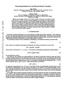
Figure 1: Comparison of TVDFT order tracking with re-sampling method. Figure 1 shows that all three of the methods agree reasonably well. The re-sampling method and the constant order bandwidth TVDFT give almost identical estimates of the order. The TVDFT methods are not compensated with the OCM, demonstrating that in many cases the TVDFT does not need to be compensated. ANALYTICAL EXAMPLE WITH RESONANCES - Analytical data was generated with a fairly large number of orders, orders 1-8 and orders 5.5 and 6.5. The rpm in this example ramps from approximately 800 rpm to 4400 rpm in 30 seconds as a squared function of time. This type of rpm profile may be typical of data acquired on a chassis dynamometer. This dataset contains 3 resonances to evaluate the performance of the order tracking methods when the amplitudes of the orders change very rapidly. A waterfall plot of this dataset is shown in Figure 2.
Figure 2: Waterfall plot fast slew rate data. As can be seen in Figure 2, the orders are very close together at low rpm values. The amplitudes of the orders also appear to change very rapidly as the orders
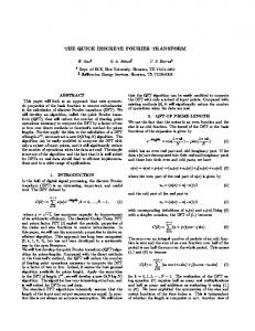
Figure 3: Waterfall plot of re-sampled angle/order domain data. The order estimates of order 5.5 are shown in Figure 4. It can be seen in this figure that the three order tracking methods used, the TVDFT frequency and order bandwidth and the re-sampled method, all agree very well except at the resonances. The differences in the estimates at the resonances are due to the fact that the amplitude of the order changes very rapidly at this point. As was pointed out earlier in this paper, all of the Fourier transform methods estimate the average amplitude of a signal over the total sample time. This property results in a larger estimate of the low frequency resonance by the TVDFT frequency bandwidth method than was obtained by either of the other two methods, due to the fact that it is averaging over a shorter time at the low rpm values. The TVDFT order bandwidth and the re-sampling methods both result in a higher amplitude estimate at the high frequency resonance because they are averaging over a shorter time at the high rpm values. This example clearly shows the time/frequency tradeoff which the different methods exhibit. Note that the TVDFT order bandwidth and the re-sampling method give nearly identical order estimates.
All of the orders present were tracked using the TVDFT constant order bandwidth method without any compensation and with OCM compensation. The results of the order tracking without compensation is shown in Figure 6.
10 TVDFT - Order Bandwid th TVDFT - Frequency Bandwidth Re-Sampling Method
0
-10 -20 Accele ration (dB) -30
140 -40
130 -50
120 Amplitude 110
-60
-70 500
1000
1500
2000
2500 RPM
3000
3500
4000
4500
Order 3 Order 3.1 Order 1 Fan Order 2 Fan
100 90 80
Figure 4: Order estimates of order 5.5.
70
ANALYTICAL EXAMPLE WITH OCM - An analytical dataset was generated with both closely spaced and crossing orders. This dataset contains orders 3 and 3.1 which would be typical of a drive axle gearset. This dataset also has constant frequency orders which would be consistent with an electric fan in an automobile. The rpm was swept from approximately 900 rpm to 4500 rpm in a period of 16 seconds. This is a common sweep rate for a vehicle on the road. The orders of the sweeping shaft as well as the orders of the constant frequency shaft were tracked both with and without OCM compensation. A Hanning window was used with a constant order bandwidth of .05 as defined by the sweeping frequency shaft. This implies that the 3 and 3.1 orders should be barely separable with the TVDFT method without OCM compensation.
60 1000
A waterfall plot of the data is shown in Figure 5. Note that the closely spaced orders cannot be visually separated and that all of the sweeping orders interact with the constant frequency orders at the crossing rpms.
Figure 5: Waterfall plot of dataset with closely coupled and crossing orders.
1500
2000
2500 3000 RPM
3500
4000
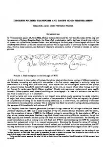
Figure 6: TVDFT constant order bandwidth order estimates without compensation. Note the inability of the TVDFT to separate completely the close orders. The bottom curve is order 3.1 which should be 40 dB below order 3. The TVDFT cannot account for any of the interaction between the crossing orders. The re-sampling and FFT based methods would give results similar to these. The results of the order tracking with compensation are shown in Figure 7. Note the ability of the OCM to separate the close orders and to compensate for the order crossings almost perfectly for all orders. This shows that the compensation effectively increases the ability of the TVDFT method to both separate closely spaced orders and to compensate for interactions between crossing orders simultaneously.
separate close orders with the OCM compensation can exceed what at first glance seems to be possible.
140 130 120
CONCLUSION
110 Amplitude 100
Order 3 Order 3.1 Order 1 Fan Order 2 Fan
The basic theory and application of the two most commonly used order tracking methods, FFT and resampling based methods, were presented. The limitations of these two methods were discussed and a basis for the development of a new algorithm established.
90 80 70 60 1000
1500
2000
2500 3000 RPM
3500
4000
Figure 7: TVDFT constant order bandwidth estimates with OCM compensation. The effectiveness of the OCM compensation is somewhat determined by how rapidly the amplitude of the orders change and how much interaction there is between orders. This limits the sweep rate which may be used to process data accurately. If the same set of orders is constant in amplitude instead of varying in amplitude, orders as close as 3 and 3.02 can be separated perfectly, even if order 3.02 is 60 dB below order 3 in amplitude. There is also perfect compensation for the crossing order interaction. These results are shown in Figure 8. 50 40 30 Amplitude 20 Order 3 Order 3.02 Order 1 Fan Order 2 Fan
10 0
The time variant discrete Fourier transform (TVDFT) was then developed and its application discussed. The basis of the TVDFT was shown to be a kernel whose frequency matched that of the tracked order at each instant in time. The TVDFT was shown to be applicable for tracking orders with either a constant frequency or constant order bandwidth. The TVDFT was shown to produce results which very closely matched the re-sampling based methods for a constant order bandwidth analysis. The TVDFT method may also be used to track order or frequency components in pass-by noise applications where a Doppler shift is present. The TVDFT was then extended through the application of an orthogonality compensation matrix (OCM), which may be applied to improve the accuracy of order estimates. The OCM is applicable where the transform kernels of the tracked orders are not perfectly orthogonal. The OCM was also shown to extend the capabilities of the TVDFT to separate contributions of closely spaced orders and crossing orders. This capability is unmatched by either the FFT or the resampling based methods. It was shown that the improvements possible with the OCM compensation were dependent on the rate of change of the amplitudes of the orders and the amount of interaction between the orders. The limitations of the OCM are a topic of ongoing research.
-10 -20 1000
1500
2000
2500 3000 RPM
3500
4000
Figure 8: TVDFT constant order bandwidth estimates with OCM compensation. Nearly the same sweeping orders as shown in Figure 6 were also tracked without the presence of the crossing orders. In this case, orders as close as 3 and 3.05 could be separated accurately. Remember, a Hanning window with a constant order bandwidth of .05 was used. This should result in a minimum separation of close orders of approximately .1 due to the window shape. This example thus shows that the ability to
REFERENCES [1] J. Leuridan , H. Vold, G. Kopp, and N. Moshrefi, "High Resolution Order Tracking Using Kalman Tracking Filters - Theory and Applications" , Proceedings of the SAE Noise and Vibration Conference, Traverse City, MI., 1995, SAE paper no. 951332. [2] J.S. Bendat and A.G. Piersol, “Random Data, Analysis and Measurement Procedures”, 2nd Edition, Wiley-Interscience, New York, pp411-417, 1986. [3] P. Van de Ponseele, H. Van der Auweraer, and M. Mergeay, “A Global Approach to the Acquisition and
Analysis of Harmonic Waveforms”, Proceedings of International Modal Analysis Conference 7, Las Vegas, NV., pp.1290-1299, 1989. [4] R. Potter and M. Gribler, “Computed Order Tracking Obsoletes Older Methods”, Proceedings of the SAE Noise and Vibration Conference, Traverse City, MI., 1989, SAE paper no. 891131. [5] P. Van de Ponseele, H. Van der Auweraer, and M. Mergeay, “Performance Evaluation of Advanced Signature Analysis Techniques”, Proceedings of International Modal Analysis Conference 7, Las Vegas, NV., pp.154-158, 1989. [6] L. Rabiner and B. Gold, “Theory and Application of Digital Signal Processing”, Prentice Hall International, London, pp.390-399, 1975. [7] J.R. Blough, D.L. Brown, and H. Vold, “Order Tracking with the Time Variant Discrete Fourier Transform”, Proceedings of the International Seminar of Modal Analysis - 21, Leuven, Belgium, 1996. [8] H. Vold and J. Leuridan, "High Resolution Order Tracking at Extreme Slew Rates, Using Kalman Tracking Filters", Proceedings of the SAE Noise and Vibration Conference, Traverse City, MI., 1993, SAE paper no. 931288.