Discrete Systems and Signals on Phase Space 1 Introduction

Applied Mathematics & Information Sciences – An International Journal c °2010 Dixie W Publishing Corporation, U. S. A.

4(2) (2010), 141–181

Discrete Systems and Signals on Phase Space Kurt Bernardo Wolf Instituto de Ciencias F´ısicas, Universidad Nacional Aut´onoma de M´exico Av. Universidad s/n, Cuernavaca, Morelos 62251, M´exico Email Address: [email protected] Received January 10, 2010

The analysis of discrete signals —in particular finite N -point signals— is done in terms of the eigenstates of discrete Hamiltonian systems, which are built in the context of Lie algebras and groups. These systems are in correspondence, through a ‘discrete-quantization’ process, with the quadratic potentials in classical mechanics: the harmonic oscillator, the repulsive oscillator, and the free particle. Discrete quantization is achieved through selecting the position operator to be a compact generator within the algebra, so that its eigenvalues are discrete. The discrete harmonic oscillator model is contained in the ‘rotation’ Lie algebra so(3), and applies to finite discrete systems, where the positions are {−j, −j+1, . . . , j} in a representation of dimension N = 2j + 1. The discrete radial and the repulsive oscillator are contained in the complementary and principal representation series of the Lorentz algebra so(2, 1), while the discrete free particle leads to the Fourier series in the Euclidean algebra iso(2). For the finite case of so(3) we give a digest of results in the treatment of aberrations as unitary U(N ) transformations of the signals on phase space. Finally, we show twodimensional signals (pixellated images) on square and round screens, and their unitary transformations. Keywords: Hamiltonian systems, Quantum mechanics, discrete signals.

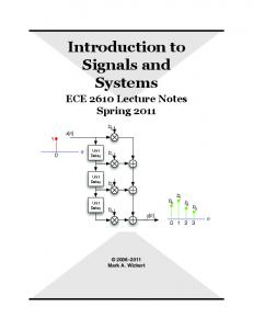
1 Introduction There has been growing interest in discrete and finite Hamiltonian systems to describe models of N -level atoms, mechanical and crystal lattices, granular versions of quantum mechanics, as well as discrete polynomials and special functions in pure mathematics. Our motivation has been to describe the parallel processing of N -point signals by unitary transformations that mimic lossless geometric optical setups, such as is sketched in Figure 1.1. Also, N 2 -point two-dimensional images on screens that are pixellated following Cartesian or polar coordinates.

142

Kurt Bernardo Wolf

z

m Figure 1.1: Sketch of an optical setup contained in a transparent microchip, where a five-point complex light signal is transformed without loss to a corresponding array of five sensors. Such a discrete Hamiltonian system is expected to register up to five momenta (ray inclinations) and carry five energy states.

Since the mid-1960s, the Fast Fourier transform (FFT) algorithm, which has O(N log N ) complexity, has allowed the real-time frequency analysis of streaming discrete data, so it has been natural to search the extension of the discrete Fourier transform (DFT) to linear canonical transformations (LCT), which for continuous systems are well understood in the context of quantum mechanics [36, 37, 58, Chapt. 9–10] and optics [23, 45]. Already the group of fractional DFT (FrDFT) presents problems when one asks only that it contain the four powers of the DFT matrix and be unitary [45, Chapt. 6], because it is not uniquely defined from those requirements [41, 69]. Nevertheless, since discrete LCTs are important for signal analysis under Fresnel and discrete-chirp transforms, efforts have been made to find efficient O(N log N ) algorithms to include the FFT in their computation [32, 48]. In Cuernavaca we have worked with Lie algebras and groups in several of its applications, among them in geometric optics on phase space [63] and in discrete models of quantum mechanics [16]. They are related through a quantization process which is distinct from the standard Schr¨odinger quantization of classical mechanics. The discrete quantization process is designed to preserve the geometry and dynamics of the geometric optical model determined by its two Hamilton equations, and to contract to the classical or Schr¨odinger quantum models under well-defined limits. The classical systems that we discretize are the harmonic oscillator, the repulsive (or inverted) oscillator, and the free particle, according to the Lie algebra that we choose. There is a corresponding phase space of the dimension of the algebra, foliated into quadratic surfaces when definite representations are chosen [1, 6], and which limit to the symplectic plane of the classical models, or to the Wigner-function formalism of quantum mechanics. In this essay we review the process of discrete quantization as a deformation of the Lie algebra of Poisson brackets between position x, momentum p, and quadratic Hamiltoni-

Discrete Systems and Signals on Phase Space

143

ans h(σ) = 21 (p2 + σx2 ), σ ∈ {+1, 0, −1}, to the three-dimensional Lie algebras so(3), so(2, 1), or iso(2), with commutators between hermitian matrices that represent the observables of position X, momentum P, and a (shifted) Hamiltonian K. The matrices will be of finite dimension N × N in the first algebra, and infinite in the second two. Exponentiated, they generate unitary matrices that form the groups SO(3), SO(2, 1) or ISO(2), of ‘translations’ in phase space and in time. Prominently, SO(3) is used in quantum angular momentum theory, where these transformations are rotations in the space of a multiplet of N = 2j + 1 states (j ∈ Z0+ , non-negative integer), such as the spherical harmonics of angular momentum j; the components of these multiplets will be here the entries of the signal N -vectors. In SO(2, 1) the multiplets are infinite, while in ISO(2) they are plainly the Fourier coefficients of periodic functions. Under these Lie algebra deformations, the classical phase space (x, p) ∈ R2 deforms to quadratic surfaces within a meta-phase space (x, p, κ(σ) ) ∈ R3 , namely a sphere, a hyperboloid, or a cylinder, respectively. A covariant Wigner function can be defined on these manifolds with all its desirable properties. The results will apply not only for signals represented by column N -vectors, but to density matrices of entangled states, under bilateral group action. In Section 2 we detail the discrete quantization process for the three systems that classically have quadratic Hamiltonians, under the ægis of the Lie algebras so(3), iso(2), and so(2, 1). We then review the ranges that the discrete position can have within each of these algebras in Section 3, their relation with the value of the Casimir invariant, and we verify that the contraction of the algebras returns the standard continuous quantum and classical systems. The overlaps between the position and energy bases provide the wavefunctions of the discrete system, and in Section 4 we find the finite difference ‘Schr¨odinger’ equations that rule the three systems. In Section 5 we write out the so(3) case of finite signals, where Kravchuk functions are the finite counterparts of the Hermite-Gauss eigenfunctions of the harmonic oscillator. The two so(2, 1) cases are given in Section 6: the discrete radial oscillator in the complementary series of representations, and the discrete repulsive oscillator model. In a short Section 7 we relate the Euclidean algebra iso(2) of a free particle to the ordinary Fourier series analysis. With these tools we examine in Section 8 the linear transformations of N -point signals in SO(3), as a subgroup of the group U(N ) of all their unitary transformations; those outside SO(3) count all possible aberrations of finite signals. Their nonlinear action is analyzed in the spherical phase space of finite systems, by means of the SO(3) covariant Wigner function that is detailed in the Appendix. In Section 9 we construct two-dimensional discrete Hamiltonian systems, modeled by finite screens pixellated along Cartesian and along polar coordinates. We define the Kronecker basis of each pixellation, and bases of definite mode and angular momentum; these correspond to Hermite-Gauss and Laguerre-Gauss beams, and their overlap involves the Clebsch-Gordan coefficients. We apply this to rotate unitarily Cartesian-pixellated images, and to map these on polar-pixellated screens, also unitarily. The concluding Section 10

144

Kurt Bernardo Wolf

returns to the context of our research on discrete systems and offers some unsolved problems. The subjects covered in this essay were presented at the International Conference on Mathematics and Information Security (Sohag, Egypt, November 13–15, 2009). This is the reason for the proliferation of citations to the author’s work in the bibliography —which is surely incomplete—, and for which I apologize.

2 Geometry and Dynamics in Discrete Quantization Recall that classical Hamiltonian systems are described by observables of position and momentum x, p, whose basic Poisson bracket is {x, p} = 1,

(2.1)

which is skew-symmetric, linearly distributive, and obeys the Leibnitz rule, so it can be extended to all differentiable functions of x, p in the form {f1 , f2 }(x, p) =

∂f1 (x, p) ∂f2 (x, p) ∂f1 (x, p) ∂f2 (x, p) − . ∂x ∂p ∂p ∂x

(2.2)

Since in particular {x, 1} = 0, {p, 1} = 0, the quantities x, p, 1 form a basis for the Heisenberg-Weyl Lie algebra w [57]. The three systems of our immediate interest are ruled by the quadratic Hamiltonian functions    +1, harmonic oscillator, (σ ) 2 1 2 h := 2 (p + σx ), σ = (2.3) 0, free particle,   −1, repulsive oscillator, that determine the two Hamilton equations, geometric: dynamic:

{h(σ) , x} = −p, {h

(σ )

, p} = σx.

(2.4) (2.5)

The first equation (2.4) is geometric because it is true for any classical Hamiltonian of the general form hV = 12 p2 + V (x), while the second equation (2.5) is dynamic because in the general case the right-hand side will be dV (x)/dx. The right-hand side of (2.5) is linear in x, p, κ(σ) (and 1) only for Hamiltonians with quadratic potentials, so only these can be the generators of a Lie algebra. For σ = +1, this algebra is the semidirect product of w with rotations so(2); for σ = −1, it is with Lorentz boosts so(1, 1), and for σ = 0 with translations iso(1). We postulate the following correspondence between the classical observables and (noncommuting) operators in some Hilbert space, with the notation position x ↔

X ≡ L0 ,

(2.6)

Discrete Systems and Signals on Phase Space

momentum

p ↔

(pseudo) energy κ(σ) ↔

145

P ≡ L1 ,

(2.7)

K(σ) ≡ L(2σ) ,

(2.8)

and 1 ↔ 1 . We shall call K the pseudo-energy —or mode— operator because the usual Schr¨odinger energy will be the eigenvalue of K + γ1 (with γ to be determined). And now we replace Poisson brackets of classical coordinates u, v, w, with commutators of operators U, V, W, through {u, v} = w ↔ [U, V] = iW, so that the two Hamilton equations (2.4) and (2.5) translate to [L(2σ) , L0 ] = −iL1 , (σ )

[L2 , L1 ] = iσ L0 ,

i.e., i.e.,

[K(σ) , X ] = −iP, [K

(σ )

, P] = iσ X .

(2.9) (2.10)

The second crucial postulate will be now set in place: the deformation of the classical algebras is performed by replacing the basic Poisson bracket (2.1) with the non-standard commutator [L0 , L1 ] = −iL2 ,

i.e.,

[X , P] = −iKσ .

(2.11)

The three operators (2.6)–(2.8), with their commutators (2.9)–(2.11), form bases for the following Lie algebras: so(3)

for σ = +1, discrete harmonic oscillator,

(2.12)

so(2, 1)

for σ = −1, discrete repulsive oscillator,

(2.13)

for σ = 0,

(2.14)

iso(2)

discrete free particle,

in direct sum with the central generator 1. The third postulate is to choose the position operator L0 ≡ X to be a compact generator in each algebra (and in its corresponding Hilbert space). The Lie-algebraic structure then ensures that its spectrum will be discrete, i.e., that the (observable) positions in the system form a collection of equally-spaced points, m ∈ Z, finite in so(3) and infinite in the other two cases [29].

3 Representations, Contractions and Energy The representations of the Lie algebras (of vector basis X , P, K(σ) ) are their realizations by matrices (X, P, K(σ) ), and we are interested in the hermitian irreducible ones, that is, those which cannot be further reduced by similarity into diagonal blocks. For the three three-dimensional algebras listed above, their characterization is obtained using the invariant Casimir operators, C (σ) := σX 2 + P 2 + K2 = σL20 + L21 + L22 = γ1 ,

(3.1)

146

Kurt Bernardo Wolf

where the value of γ essentially determines the irreducible representation (for so(2, 1) an extra dichotomic index is necessary). These matrices act on column vectors, the discrete wavefunctions that we may also call signals, or states of the system. The states live in complex Hilbert spaces of square-summable sequences `2 over the integers Z, or over Z0+ , or CN for finite dimension N , with the usual inner product and norm, X √ ∗ (f, g) := fm gm = (g, f )∗ , |f | := (f, f ), (3.2) m∈Σ(X )

where Σ(X ) is the spectrum of X . The simultaneous eigenbasis of the compact position generator of the algebra, X = L0 , and of the Casimir operator (3.1), is the Kronecker basis for the system, γ γ X fm = m fm ,

m ∈ Z,

γ γ C (σ) fm = γ fm ,

(3.3)

so {fm }m∈Σ(X ) are column vectors of 0’s with a single 1 at position m. For the three algebras under consideration, the spectra {γ} = Σ(C (σ) ) and {m} = Σ(X ) are [22, 29, 42] so(3) σ=1 so(2, 1) σ = −1

γ = j(j + 1), j ∈ Z0+ , |m| ≤ j, representation of dimension N = 2j + 1;

(3.4)

γ = k(1 − k) < 14 , k ∈ Z + , k complementary series D± ,

(3.5)

γ = k(1 − k) ≥ 14 , principal series C0κ ; iso(2) σ=0

m ∈ ±{k, k+1, . . .},

k = 12 +iκ, κ ∈ R,

m ∈ Z,

γ = l2 , l ∈ R, m ∈ Z, infinite-dimensional representation.

(3.6)

(3.7)

This list is incomplete because when these Lie algebras are exponentiated to the cor1:2 1:2 responding Lie groups, they have covers: SO(3) = SU(2), SO(2, 1) = SU(1, 1) = 1:∞ 1:∞ Sp(2, R) = SL(2, R) = Sp(2, R), and ISO(2) = ISO(2). The first, SU(2), can have also half-integer {m} spectra, while the infinite covers exhibit integer-spaced m’s on any real values (additionally, SO(2, 1) has the supplementary series in the interval 0 < k < 1). We shall thus only consider representations where m = 0 is a position point of the discrete system. As we promised above we should show that under contraction, when the discrete position points come closer together until they are dense in the continuum, the discrete systems described by (3.4)–(3.7) become the usual quantum mechanical harmonic and repulsive oscillators, and the free particle. First we prove this for the algebras, and then for the Hamiltonians. Dropping σ as superindex, let X γ := γ −1/4 X ,

P γ := γ −1/4 P,

Kγ := K + γ 1/2 1 ,

(3.8)

Discrete Systems and Signals on Phase Space

147

where γ is the value of the Casimir operator (3.1). When γ → ∞, the two Hamilton equations (2.9)–(2.10) remain invariant (as they should), while the nonstandard commutator (2.11) becomes 1 i √ −→ i1 , [X γ , P γ ] = √ [X , P] = − √ (Kγ − γ1 ) γ→∞ γ γ

(3.9)

weakly, in the subspace of `2 states f = {fm } such that (f, K2 f ) < ∞, i.e., signals of bounded energy as defined below. Next, we write (3.1) as γ1

= =

=⇒

√ √

√ √ γP 2γ + σ γX 2γ + (Kγ − γ1 )2

γ(P 2γ + σX 2γ − 2Kγ ) + K2γ + γ1 , 1 Kγ = 12 (P 2γ + σX 2γ ) + √ K2γ , 2 γ

(3.10) (3.11)

which becomes the Schr¨odinger version of (2.3), with the same condition of validity. This also indicates that the eigenvalues η of Kγ are related to the eigenvalues λ of K through √ Kγ = K + 1 γ. Thus, the relation between energy and pseudo-energy has the generic form √ η ≈ λ + γ + constant. (3.12)

4 ‘Schr¨odinger’ Difference Equations Continuous quantum mechanical systems evolve obeying Schr¨odinger second-order differential equations, which are determined by their Hamiltonian, where the momentum operator is realized as −i~d/dx, and position by x, which thus relate three infinitesimally near points of space. The discrete systems introduced here are a pre-contracted version of those, and so obey a finite difference equation that relates the values, in each pseudo-energy eigenstate, of three neighboring points spaced by unity, K hγλ = λ hγλ ,

λ ∈ Σ(K),

C hγλ = γ hγλ .

(4.1)

The wavefunctions of the discrete system will then be the overlaps between the Kronecker position eigenbasis (3.3) and the energy basis (4.1), namely γ Ψγλ (m) := (fm , hγλ ).

(4.2)

To find this ‘Schr¨odinger’ difference equation, one uses the raising and lowering operators L↑ := K + iP, L↓ := K − iP. (4.3) From (2.9)–(2.11), their commutators are [L0 , Ll ] = ±Ll and [L↑ , L↓ ] = 2σL0 . Their role is to shift the position of the Kronecker states (3.3) up and down by one unit, γ γ L↑↓ fm = cγ↑↓ m fm±1 .

(4.4)

148

Kurt Bernardo Wolf

The normalization constants cγ↑↓ m can be found through a well-known line of reasoning [29] that involves writing the Casimir invariant (3.1) as C = L↑↓ L↓↑ + L0 (L0 ± 1 ) and γ applying it to fm . The result is p p (4.5) cγ↑ m = ϕ↑ m γ − σm(m+1), cγ↓ m = ϕ↓ m γ − σm(m−1), with phases that can be of the general form ϕ↑ m = eiαm and ϕ↓ m = e−iα(m−1) , with α modulo 2π at our choosing, but subject to convention [22, 29] to α = 0. Then, (4.1) and (4.4) with 2K = L↑ + L↓ , lead to the following three-term difference equation in discrete position p p γ − σm(m+1) Ψγλ (m+1) + 2λΨγλ (m) + γ − σm(m−1) Ψγλ (m−1) = 0. (4.6) This difference equation contracts under (3.8)–(3.12) to the Schr¨odinger equations: denoting the eigenvalues of X by m, those of X γ by x := γ −1/4 m, and re-defining ψ (x) = ψ(γ −1/4 m) := Ψγλ (m), for γ large and δ := γ −1/4 , we expand (4.6) to order δ 2 and approximate using x-derivatives, Ψγλ (m ± 1) = ψ(x ± δ) ≈ p γ − σm(m±1) ≈

ψ (x) ± δ ψ 0 (x) + 21 δ 2 ψ 00 (x), √ γ − 12 σx2 ∓ δ σx − 81 δ 2 x4 .

(4.7) (4.8)

Replacing into (4.6) and truncating to order δ 2 , the γ → ∞ limit is 00 1 2 (−ψ (x)

+ σx2 ψ (x)) = (λ +

√

γ) ψ (x) = η ψ (x),

(4.9)

i.e., the time-independent Schr¨odinger equation of the corresponding quadratic system. In the following sections we shall show separately the wavefunctions of the three onedimensional systems of our concern: the finite so(3) harmonic oscillator, the two so(2, 1) cases of the discrete radial and repulsive oscillators, and the iso(2) discrete free particle. Then, their respective phase spaces will be given, and finally some comments on the current progress in two-dimensional images will be cited.

5 The so(3) Finite Oscillator The Lie algebra so(3) is the only compact three-dimensional one, and the finite harmonic oscillator thus serves for the analysis of N -point finite signals {Fm } = F ∈ CN of complex values. We shall treat N = 2j + 1 to be an odd number (j positive integer) with a symmetric range of positions −j ≤ m ≤ j, so that the center m = 0 be in the sensor set. The difference equation (4.6) can be compared with the solutions to the standard Wigner so(3) recursion relation [22, Eqs. (3.83)], p p (j−m)(j+m+1) ψλj (m+1) + 2λψλj (m) + (j+m)(j−m+1) ψλj (m−1) = 0, (5.1)

Discrete Systems and Signals on Phase Space

149

where the coefficient of ψλj (m+1) vanishes for m = j and that of ψλj (m−1) for m = −j, so that the discrete oscillator wavefunctions are zero for |m| > j. The coefficients that relate the spherical harmonics refered to two colatitude axes separated by an angle β are the Wigner little-d functions djm,m0 (β); in our case, the position and energy axes, x- and κ, are orthogonal; we thus recognize the solutions of the difference equation (5.1) to be Ψjn (m) :=

djλ,m ( 21 π)

n := λ + j ∈ [0, 2j]

(5.2)

n

= =

(−1) (2j)! 2 F1 (−n, −2j−m; −2j; 2) p 2j n! (2j−n)! (j+m)! (j−m)! s (−1)n ³ 2j ´³ 2j ´ Kn (j+m; 12 , 2j). n j+m 2j

(5.3) (5.4)

The discrete position coordinate is −j ≤ m ≤ j, the state mode is n, and energy (3.12) is η := n + 21 [16]. The expression (5.4), found by Atakishiyev and Suslov [15], factors the m-dependence of the Wigner-d into a symmetric Kravchuk polynomial of degree n [14,15], Kn (j+m; 21 , 2j) = 2 F1 (−n, −2j+m; −2j; 2) = Kj+m (n; 12 , 2j),

(5.5)

and the square root of a binomial. When contracted by j → ∞, the former become Hermite √ polynomials and the latter a Gaussian factor. As shown in [12], upon writing m = x j, .p 2 √ lim (−1)m j 1/4 Ψjn (m) = e−x /2 Hn (x) 2n n! π. (5.6) j→∞

We will refer to {Ψjn (m)}2j n=0 as the modes of the finite harmonic oscillator. Please note that in the overlap (4.2) and in the ensuing discussion leading to the difference equation (5.1), we can permute the axes {Li } through 0 → 2 → 1 → 0, and thus obtain a difference equation relating three neighboring energy wavefunctions, Ψjn (m) and Ψjn±1 (m), exchanging only m ↔ λ = n − j; i.e., Ψjn (m) = Ψjm+j (n − j ). The Wigner little-d’s have many symmetry and other properties. In particular note carefully that for integer n ∈ [0, 2j], Ψjn (m) is an analytic function of m —being the product of a polynomial and the square root of a binomial— with branchpoint zeros at the integers |m| > j. Conversely, for integer |m| ≤ j, it is a similar analytic function of n. In Figure 5.1 we show the finite harmonic oscillator wavefunctions Ψjn (m) for N = 65 points {m} and selected numbers n near to the bottom, center and top of this j = 32 multiplet. These wavefunctions are real, orthogonal and complete in CN . Another useful representation of the whole basis is provided by a density plot of the matrix Ψj = kΨjn (m)k, shown in Figure 5.2; as we remarked above, this matrix is symmetric across the diagonal. The finite oscillator wavefunctions form a privileged basis from which a density-matrix description of entangled states can be made. Under SO(3) rotations, the states (5.2) will transform among themselves irreducibly, with the same Wigner ‘big-D’

150

Kurt Bernardo Wolf

n = 64

m

63

62

32

2

1

0.5

n=0

m 30

20

10

10

20

30

0.5 Figure 5.1: Finite oscillator wavefunctions Ψjn (m) for N = 65 points. From bottom to top, n = 0, 1, 2, . . . , 32, . . . , 62, 63, 64 = 2j.

j coefficients Dm,m 0 (α, β, γ) as the spherical harmonics [29]. Time evolution is generated by exp[−iτ (K + j + 21 )], which multiplies Ψjn (m) by the phase exp[−iτ (n + 21 )].

151

Discrete Systems and Signals on Phase Space

16

0

-16 0

32

Figure 5.2: The finite oscillator basis represented through the density plot of the matrix kΨjn (m)k, on the horizontal axis n ∈ [0, 2j], and vertical axis m ∈ [−j, j], for j = 16, i.e., for 2j + 1 = 33-point systems.

The ground state of the finite oscillator is s Ψj0 (m)

=

dj−j,m ( 21 π)

1 = j 2

(2j)! , (j+m)! (j−m)!

(5.7)

while the top state Ψj2j (m) = (−1)m Ψj0 (m) is the highest-energy waveform that the finite system can carry. As with the quantum oscillator ground state, all coherent states are obtained through translation —here SO(3) rotation— of phase space [14, 69]. This indicates that a sphere will be the proper phase space for finite hamiltonian systems, as we shall elaborate below, after we present the wavefunctions of the SO(2, 1) and ISO(2) discrete systems. Another point which merits consideration is that the finite oscillator difference equation (5.1), stemming from K = 21 (L↑ + L↓ ), does not separate into a sum of kinetic and potential energy terms. However, an ‘equivalent potential’ can be defined from (5.7), since the ground state has no zeros, as its normalized second-difference ∆Ψj0 (m)/Ψj0 (m). As expected, this yields a parabola-like discrete form [62].

6

The Two so(2, 1) Cases

so(2, 1) is a non-compact Lie algebra; the representative of its only compact generator will be the position operator X whose spectrum is discrete; the pseudo-energy operator

152

Kurt Bernardo Wolf

K can have discrete or continuous spectra according to the eigenvalue γ = k(1 − k) of k the Casimir operator [see (3.7)], in the complementary lower-bound D+ when γ < 41 (extended to continuous k > 0); or in the principal C0κ series of so(2, 1) representations when γ ≥ 14 , k = 21 + iκ (κ ∈ R). The two cases have been investigated in different k contexts. First, for D+ in (3.5), we give the results of Ref. [9] regarding a discrete radial harmonic oscillator (or a one-dimensional oscillator with centrifugal force). And second, for C0κ in (3.6), we return with the discretization philosophy applied to the one-dimensional repulsive oscillator system following Ref. [39]. 6.1

Discrete radial oscillator

The framework for a discrete analogue of the radial part of a D-dimensional harmonic oscillator is based on the group of linear canonical (symplectic) transformations of ordinary quantum-mechanical phase space [38, 56], reduced with respect to D-dim rotations, Sp(2D, R) ⊃ SO(D) ⊗ Sp(2, R).

(6.1)

On the right-hand side, the two groups are complementary, i.e., within one representation of Sp(2D, R), the representation of the angular subgroup SO(D), determines the representation of the radial subgroup Sp(2, R). In the plane D = 2 case, the rotation subgroup is SO(2) with eigenfunctions ∼ eiaφ , integer a being the angular momentum; but its infinite cover SO(2) is the translation group, where a can be real. Separating the continuous variables of radius r ∈ R+ from angle φ, the Hamiltonians of the three quadratic systems we are treating generate a realization of the ‘radial’ Lie algebra so(2, 1) ≡ sp(2, R), given by second-order differential operators,1 (k) Jb0 :=

1 4

³

´ a2 − 41 d2 2 + + r , dr2 r2 ³ d ´ (k) Jb2 := −i 12 r + 21 , dr −

(k) Jb1 :=

1 4

³ −

a2 − d2 + dr2 r2

1 4

´ − r2 , (6.2)

(k) (k) (k) i.e. Jb− := Jb0 − Jb1 = 12 r2 .

(6.3)

The relation between a ≥ 0 and the Bargmann index k is evinced by the Casimir operator (3.1) of this realization, Cb = γ1 , for

γ = 41 (1−a2 ) = k(1−k), a = 2k−1, k := 12 (a+1) ≥ 12 ,

(6.4)

exactly as in (3.5). These operators are essentially self-adjoint in a Hilbert space L2 (R+ ) with measure dr. They exponentiate into the group of unitary ‘radial’ canonical integral transformations (including fractional Hankel transforms), whose complex extension was analyzed in [56]. 1 Classical Lie theory deals only with first-order differential operators; the only semisimple algebras one can realize with second-order differential operators are the real symplectic algebras of dimension D.

Discrete Systems and Signals on Phase Space

153

(k) The compact generator 2Jb0 in (6.2) is a harmonic oscillator plus a centrifugal potential C/r2 , with coefficient C := a2 − 41 ≥ − 14 for k ≥ 12 . In so(2, 1), the exceptional interval is 0 ≤ k < 1, which includes weak barriers 0 < C < 34 , weak wells − 41 < C < 0, and C = 0; in this interval, the operators do not have a unique self-adjoint extension, but again we simplify matters by taking the Friedrichs extension, where the spectrum of this (k) oscillator + centrifugal Hamiltonian 2Jb0 is equally spaced and given by η := n + k, (k) n ∈ Z0+ [66]. For all representations the ‘square-radial’ position operator is Jb− = 21 r2 in (6.3), which is diagonal, non-compact, and with a simple spectrum 12 r2 ≥ 0 for r ≥ 0. The (k) eigenfunctions of 2Jb0 in this realization are the well-known Laguerre-Gauss functions that will appear below [in (6.12)]. We do want equally-spaced energies, but to have a discrete system, we must choose (k) (k) some other compact so(2, 1) generator —distinct from Jb0 but with a limit to Jb− — to be our square-radial position operator. This we can achieve with a diagonal scaling transform [9], defining for every k and ζ > 0, the ‘discrete square-radial’ operators

Jb(ζ)

:= =

e−ζ exp(iζ Jb2 ) Jb0 exp(−iζ Jb2 ) ³ d2 a2 − 14 ´ 1 2 + 4r , e−2ζ 14 − 2 + dr r2

(6.5)

whose ζ → ∞ limit is clearly Jb(∞) = 21 Jb− = 14 r2 . The overlaps between the eigenfunctions of energy, ψnk of 2Jb0 with eigenvalue λ = k k + n (n ∈ Z0+ ), and the Kronecker eigenbasis of position, ψζ,m of 2Jb(ζ) , with eigenvalues + 2 −ζ µ = k + m (m ∈ Z0 ), on the square-radial positions rm ≈ 2e m ≥ 0, are Ψk,ζ n (m)

:= =

k (ψζ,m , ψnk ) k k (exp[iζ Jb2 ]ψm , ψnk ) = (ψm , exp[−iζ Jb2 ]ψnk )

(6.6) (6.7)

To find this overlap, we use the raising and lowering operators as in (4.3) with the Jbi ’s instead of Li ’s, and follow (4.4)–(4.6) to find the difference equation for Ψk,ζ n (m) that relates three neighboring points in space, m and m ± 1. Recalling that µ := k + m and λ := k + n, this is p (m + 1)(2k + m) Ψkn (m+1) + 2(k+n) Ψkn (m) (6.8) p + m(2k + m − 1) Ψkn (m−1) = 0 We see that the second coefficient ck↓, µ=k = 0 provides the zero boundary condition for k k m < 0 in the D+ representation series (the upper-bound series D− contains all m ≤ 0). The boundary condition at zero determine uniquely the solution to (6.8), which is also known in the guise of the Bargmann SO(2, 1) little-d function dkk+m,k+n (ζ) [18]; this is none other but the unitary irreducible representation matrix of the boost between the two bases (6.6). Several expressions for it exist, among them one that displays them in

154

Kurt Bernardo Wolf

terms Meixner polynomials, found by Atakishiyev and Suslov [15]. Using the parameter ξ := tanh2 21 ζ ∈ (0, 1), this displays the discrete radial oscillator wavefunctions as Ψk,ζ n (m) := =

dkk+m,k+n (ζ) = Ψk,ζ m, n ∈ Z0+ m (n) r ξ n+m (1 − ξ)2k (2k)n (2k)m Mn (m; 2k, ξ), n! m!

(6.9) (6.10)

where (a)n = Γ(a+n)/Γ(a) is the Pochhammer symbol, and the Meixner polynomial of degree n in m is Mn (m; 2k, ξ) = 2 F1

³ −n, −m 1´ ; 1− = Mm (n; 2k, ξ). ξ 2k

(6.11)

We should be aware from (6.5) and the text below, that the discrete points m ≥ 0 now √ correspond to discrete radii rm = 2e−ζ/2 m. These functions are orthogonal and complete in the Hilbert space `2 (Z) of square-summable sequences, and form also a symmetric, but now half-infinite matrix. And again note carefully that for integer n ∈ Z0+ , Ψkn (m) is an analytic function of m with branchpoint zeros at the negative integers; and conversely for m ∈ Z0+ as a function of n. In Figure 6.1 we show discrete radial oscillator wavefunctions Ψk,ζ n (m) in (6.10) for various values of a, n, ζ, while in Figure 6.2 we show the density plot of a part of the whole, infinite basis. We understand that as ζ grows, the radii rm come closer together and the approximation to the Laguerre-Gauss wavefunctions improves. Indeed, the ζ → ∞ limit relation is [9] s 2 1 ζ/2 k,ζ 1 ζ 2 2 n! lim √ e Ψn ( 4 e r ) = e−r /2 ra+1/2 Lan (r2 ), (6.12) ζ→∞ 2 (a+n)! with a = 2k − 1. Comparing this limit with the γ → ∞ limit in (4.9) and (5.6), we see that here ζ is a contraction parameter independent of the representation. 6.2

Discrete repulsive oscillator wavefunctions

We return to the main line of reasoning to discretize quadratic Hamiltonian systems, namely (2.6)–(2.8) for the case (2.13) of the repulsive oscillator. The energy spectrum of this system is the full real line, η ∈ R, but the set of positions will be discrete and infinite, m ∈ Z, so we must use the representations (3.6) in the principal series C0κ where k = 12 +iκ and γ = κ2 + 14 , labelled by κ ∈ R. There are several reasons for investigating the discrete wavefunctions that converge to the quantum repulsive oscillator wavefunctions [58, Sects. 7.5.11–15]: it is a discrete but Dirac-orthonormal basis for `2 (Z) in the pseudo-energy label λ; there is a classical distinction between negative- and positive-energy states, which reflect or pass over the potential barrier, but tunneling should occur under quantization; the

155

Discrete Systems and Signals on Phase Space

k =1

k =1/2 n = 0

n=0

r

r 1

1 1.

1.

 0.5

1

2

3

4

5

6

 0.5

2 1

2

3

4

5

6

 0.5

3 1

2

3

4

5

6

 0.5

4

4

5

6

2 1

2

3

4

5

6

3 1

2

3

4

5

6

4

1.

1.

 0.5

3

1.

1.

 0.5

2

1.

1.

 0.5

1

1

2

3

4

5

6

 0.5

1

2

k =3/2 n = 0

3

4

k=2

5

6

n=0

r

r

1

1

1.

 0.5

1.

1

2

3

4

5

6  0.5

1

2

3

4

5

2  0.5

1.

1

2

3

4

5

6  0.5

3

1.

 0.5

1

2

3

4

5

6

3

1.

1

2

3

4

5

6  0.5

4

1.

 0.5

6

2

1.

1

2

3

4

5

6

4

1.

1

2

3

4

5

6  0.5

1

2

3

4

5

6

Figure 6.1: Eigenfunctions of the discrete harmonic oscillator with a centrifugal potential, Ψk,ζ n (m) in (6.10), with angular momenta a = 2k − 1 shown in (a): For a = 0 (k = 21 ), (b): a = 1 (k = 1), (c): a = 2 (k = 32 ). Each graph contains successive refinements of the set of orthogonality points 2 rm = 4eζ m, for ζ = 0.5, 1, 3, 5, ∞, marked by bullets of decreasing size, interpolated (since they are analytic functions of m) by dashings that converge to the continuum Laguerre-Gauss functions. From top to bottom, the radial modes n = 0, 1, 2, 3, 4.

quantum wavefunctions behave as chirps ∼ exp(iax2 ) for large x, yet discrete signals are bound by an upper frequency. The constants (4.5) in this case are all nonzero; in (4.6) they yield the difference equation q q (m+ 12 )2 +κ2 ψλκ (m+1) − 2λψλκ (m) + (m− 12 )2 +κ2 ψλκ (m−1) = 0. (6.13) This equation has two independent solutions, which may be separated into right- and left-

156

Kurt Bernardo Wolf

0 0

Figure 6.2: The discrete centrifugal oscillator basis represented through a density plot of the matrix + 1 kΨk,ζ n (m)k in (6.10), for ζ = 1, k = 2 (angular momentum a = 0), and n, m ∈ Z0 shown up to n, m ≤ 45. The figure is symmetric under n ↔ m, so the axes are exchangeable. Compare with Fig. 5.2.

moving waves, as determined by their values at two points, m = 0 and 1 for example. How to separate them? From previous work we recognize that the Ψκλ (m)’s are the overlaps between the Kronecker eigenbasis of position L0 and the Dirac basis of pseudo-energy L2 , which was computed solving integrals in Ref. [20, Eq. (4.14)], resulting in the sum of two hypergeomentric functions. Dissatisfied with this form, in [40] we proposed a change of functions and, using [30, Eq. 9.137.1], found two solutions distinguished by an inversion sign τ ∈ {+, −}, each given by a single hypergeometric function: Ψκλ,τ (m)

|Γ( 21 +iκ+τ m)| 2 F1 Γ(1−iλ+τ m)

:=

cκλ iτ m

=

Ψ−κ λ,τ (m)

=

Ψκλ,−τ (−m),

·1

1 2 −iκ−iλ, 2 +iκ−iλ ;

1−iλ+τ m

¸ 1 , (6.14) 2 (6.15)

where cκλ is an m-independent normalization coefficient that may be proposed from [20, Eq. (4.14)], but which for numerical purposes can be set to any constant value. When plotting these functions in Figure 6.3, we see that they are the right- and left-moving discrete repulsive oscillator wavefunctions [58, Fig. 7.11]) with energies η = λ + κ. The density plot of this basis in Figure 6.4 shows that the phase iτ m in (6.14) is indeed the appropriate one —otherwise the function would oscillate between neighboring positions. As for (5.6), we

157

Discrete Systems and Signals on Phase Space h= 2

k = 2

-20

k = 25

20

-40

40

k = 49

-56

56

1

0.5

0

-0.5

-1

-2

Figure 6.3: Discrete repulsive oscillator wavefunctions, Ψκλ,+ (m) in (6.14). The columns correspond to representations κ = 2, 25 and 49; the rows, to energies η = λ + κ = 2, 1, 0.5, 0, −0.5, −1, and −2. Dashed, dotted and continuous lines join the real, imaginary and absolute values of the functions √ between integer positions m, whose ranges are scaled by factors ∝ κ attending to the contraction (6.16).

expect that lim κ1/4 Ψκλ,τ (m) =

κ→∞

√ exp[i 14 π( 12 − iη)] 1 Γ( 2 −iη) D− 12 +iη (τ ei3π/4 2 x), 3/4 2 π

(6.16)

√ for m = x κ and η = λ+κ, should return the quantum wavefunctions with their parabolic cylinder functions Dν (z ). As in previous cases, the discrete wavefunctions are actually analytic in the position coordinate m (set iτ m = exp i 12 τ m.), although in this case we could not factor them into a form with some known discrete special function. Regarding the asymptotic behavior κ κ |m| → ∞, (6.13) shows that Ψλ,τ (m+1) ≈ −Ψλ,τ (m−1), so the chirp of the continuous case deforms into a highest frequency of period 4. Moreover, the use of (6.14) in numerical computations raises questions since it is a Dirac basis, so their norm is infinite. In Ref. [40] we commented on the use of N vectors Ψκλn ,τ (m) of chosen λn ’s on N positions m, as a finite non-orthogonal basis.

158

Kurt Bernardo Wolf 2

2

h

-2 -40

h

m

-2 40

-40

m

40

Figure 6.4: Density plots of the real (left) and imaginary (right) values of a (finite) discrete repulsive oscillator sub-basis Ψ25 λi ,+ (m) for 25 positions m ∈ {−12, −11, . . . , 12}, and 25 energies {ηi } equally spaced between −2 and 2.

7 The iso(2) Free Case The three-parameter Euclidean algebra iso(2) describes the discrete free particle, with σ = 0 in (3.7), on the infinite discrete position set of points m ∈ Z. The spectrum {λ} of K is evident when we realize the generators of the iso(2) algebra on the circle θ ∈ (−π, π], b := −id/dθ, Pb := l sin θ and K b = l cos θ, so λ = l cos θ and −l ≤ λ ≤ l, l ∈ R. The X eigenvalues of the Casimir operator are γ = l2 , and the recurrence relation (4.6) acquires 2 a simple form when in (4.5) cll = l. We label the iso(2) representations with l ≥ 0 and a dichotomic index υ, l Ψlλ,υ (m+1) + 2λΨlλ,υ (m) + l Ψlλ,υ (m−1) = 0.

(7.1)

The two independent solutions, distinguished by υ as parity, are 1 Ψlλ,+ (m) = √ cos(mθ), π

1 Ψlλ,− (m) = √ sin(mθ), π

(7.2)

with θ = arccos(λ/l), θ ∈ [0, π] and, according to (3.12), energy η = λ+l = l(1+cos θ) ∈ [0, 2l]. In Figure 7.1 we show the free wavefunctions (7.2), noting that since they are analytic in m, we can plot them as if the functions were continuous. The discrete free particle has thus a restricted continuous range of energies, bounded below by a constant wavefunction, and above by one with the shortest wavelength, whose √ period is 2. We may also use their complex linear combinations Ψlλ := (Ψlλ,+ +iΨlλ,− )/ 2 for θ ∈ (−π, π]; thus in essence, the iso(2) basis (7.2) provides the Fourier series decomposition between bandlimited signals f (θ) and their Fourier coefficients fm , which are interpreted as the discrete wavefunctions of a free system. The Euclidean case is well known in the model of an infinite discrete lattice of masses joined by springs, whose dynamics

159

Discrete Systems and Signals on Phase Space

m

m Figure 7.1: Discrete free particle wavefunctions, Ψlλ,+ (m) and Ψlλ,− (m) in (7.2). Recall that λ = l cos θ, so that there is actually a continuum −l ≤ λ ≤ l of energies η = λ + l; for θ = 0 and π, Ψl±l,− = 0.

is given by a Green function which is the bilinear generating function of the basis (7.2) integrated over the circle, dlm,m0 (ζ)

:= = =

(Ψl (m), exp(−iζK) Ψl (m0 ))L2S Z π 0 1 dθ exp(−iζl cos θ) ei(m −m)θ 2π −π 0

eiπ |m−m |/2 J|m−m0 | (ζl).

(7.3)

(7.4)

The Green matrices kdlm,m0 (ζ)k are here symmetric, infinite circulating matrices, whose elements depend only on the distance |m−m0 | to the main diagonal. They exhibit the group property X dlm,m0 (ζ1 ) dlm0 ,m00 (ζ2 ) = dlm,m0 (ζ1 +ζ2 ). (7.5) m0 ∈Z

160

Kurt Bernardo Wolf

Indeed, the Green matrices belong to the irreducible representation l of a translation subgroup of the Euclidean group ISO(2), and correspond to the Wigner and Bargmann littled’s of rotations and boosts in the other two three-parameter groups. The same bilinear construction can be made for the other two cases to obtain the full representation matrices of the groups in ‘Euler parametrization’ as 0

s −imα s Dm,m dm,m0 (ζ) e−im γ , 0 (α, ζ, γ) = e

(7.6)

where s stands for the j, k, l representation labels of the respective groups SO(3), SO(2, 1) or ISO(2) used previously. Conversely, the signals Ψsλ (m) will transform linearly and irreducibly, as column vectors, under their irreducible representation matrices (7.6). The wavefunctions Ψsλ (m) are orthonormal and complete, so any signal f (m) can be decomposed into and synthesized from these mode coefficients. (We call them mode coefficients because for finite signals they provide the oscillator energy mode content.) Indicating by S the sum or integral over the range of pseudo-energies λ (the spectrum of K(σ) in the representation s of the algebra), the analysis and synthesis of the signal in the mode basis is X (7.7) f (m) Ψsλ (m)∗ , fλs = f (m) = S fλs Ψsλ (m), λ∈Σ(K,s)

x∈Σ(X ,s)

with λ(n) shifted appropriately. For ISO(2) this is the Fourier series decomposition, wellknown and well applied. But when we return to our finite model of a parallel-processing optical chip in Figure 1.1, it is the finite case that should be of special interest, because considerable labor has been expended in using bases for (7.7) with sampled and orthonormalized Hermite-Gaussian functions [48, 49], Harper functions [19], and the non-orthogonal Mehta functions [34]. Comparing these sampled bases with the Kravchuk function basis (5.4), in Ref. [65] we addressed the questions of approximation and exact restoration of a signal when one has gained access only to a few of its lowest mode coefficients; in particular the concomitant finite Gibbs phenomenon at the sharp edges of rectangle signals. There are pros and cons in both bases.

8 Group Transformations and Aberrations We turn now to extend the transformations due to the unitary action of the group elements of SO(3), SO(2, 1) or ISO(2) on the finite or infinite signal vectors, and to introduce transformations outside those groups, which are also unitary, and which follow from the discrete quantization of the Lie-Hamilton aberrations in geometric optics [24,25,59]. Most of the work done so far has been for finite, N -point signals [64], i.e., for SO(3). Certainly, as the optical model of Figure 1.1 suggests, the setup may not process the signal as a perfect harmonic oscillator, but may have aberrations [60]. In geometric optics [63, Part 4], these

Discrete Systems and Signals on Phase Space

161

aberrations are generated by nonlinear functions of the phase space coordinates x, p. For two-dimensional optics, we chose the basis of monomial power functions, M r,ω (x, p) := pr+ω xr−ω ,

(8.1)

of weight ω ∈ {−k, −k+1, . . . , k}, and of rank r ∈ { 21 , 1, 23 , . . .}. Their Poisson operators {M r,ω , ◦} act on the phase-space coordinates x, p turning them into monomial power functions of degree Ac = 2r − 1, that we call the classical aberration order. The one-parameter group of operators exp(τ {M r,ω , ◦}) thus acts nonlinearly in classical phase space. In Figure 8.1 we show these transformations. Now we can discretely quantize the functions (8.1), here generalized to the three coordinates x, p, κ of the so(3) Lie algebra generators (2.6)–(2.8), which in the representation Dj of dimension N = 2j + 1 are the following matrices, position Xm,m0

x ↔ X = kXm,m0 k =

m δm,m0 ,

=

p ↔ P = kPm,m0 k √ √ −i 21 (j−m)(j+m+1) δm+1, m0 + i 21 (j+m)(j−m+1) δm−1, m0 , (8.3)

=

h ↔ K = kKm,m0 k 1√ 1√ 0 0 2 (j−m)(j+m+1) δm+1, m + 2 (j+m)(j−m+1) δm−1, m . (8.4)

momentum Pm,m0 (pseudo) energy Km,m0

(8.2)

The position matrix X is diagonal, the matrix K is found replacing λ in (5.1), and P is obtained in the same way from (4.3), or from (2.9) by commuting [K, X] = −iP. The three matrices are hermitian and traceless; energy is represented by a real and symmetric matrix, while momentum is pure imaginary and skew-symmetric, as the Schr¨odinger operator Pb = −i d/dx is. The i-exponential of these matrices yields the representation j of the group SO(3), because their Casimir invariant is X2 + P2 + K2 = j(j + 1)1.

(8.5)

Now, to introduce aberrations on the classical x, p, κ coordinates, we associate matrices to their monomials using the Weyl product rule: xa pb hc

↔

{Xa Pb Kc }Weyl

:=

X z }| { z }| { z }| { 1 X · · · X P · · · P K · · · K, (a+b+c)! permutations

a factors b factors c factors

(8.6)

and linear combination for summands. We note that a Weyl-ordered product of hermitian matrices is hermitian, and thus the matrices (8.6) will i-exponentiate to unitary ones. It

162

Kurt Bernardo Wolf

x p

Ac = 1

2

3

4

5

=

3

5 2

2

3 2

1

1 2

0

1 2

1

3 2

2

5 2

3

Figure 8.1: Infinite tower of linear transformations and aberrations of classical phase space x, p, generated by the monomials (8.1), classified by aberration order A and weight ω. The unit map is at the top; then come Heisenberg-Weyl translations along x and p (zero aberration order). The linear Sp(2, R) transformations (Ac = 1) are free propagation, (inverse) magnification, and a Fresnel lens. Higher aberrations of orders Ac = 2, 3, 4, 5 . . . follow. In geometric optics, aligned systems produce only odd-order aberrations.

is not difficult to prove that through products and powers, the latter exhaust the full N 2 parameter Lie group U(N ) of N × N unitary matrices. Of course, aberrations should not imply loss of signal information, so they should be represented by unitary matrices. Since there cannot be more than N 2 independent N × N unitary matrices, the set of finite aberrations corresponding to (8.1) must contain redundancies. Equation (8.5) is one restriction that we choose to limit the powers of K to 0 or 1; and then we count the powers of P where the nonzero subdiagonals reach the matrix corners. In this way we can classify the generators of the U(N ) aberration group following their classification in geometric

Discrete Systems and Signals on Phase Space

163

m

Figure 8.2: The first pyramid of aberrations up to order A = 4 for an N = 21-point signal. Top: Rectangle function shown left; at right, its Wigner function, projected on the (β, γ) polar coordinates of the sphere. Second row: SO(3)-translations in position and momentum (aberration order A = 1) generated by P and −X. Following rows: aberrations of orders 2, 3, and 4. The contour lines give higher resolutions to the near-zero values of the Wigner function: 0.0, ±0.0001, ±0.001, ±0.01, 0.02, 0.03, . . . , 0.15, 0.2, 0.3, . . . , 3.0, 3.1.

optics, defining two pyramids of aberrations Mr,ω;0

:= {Pr+ω Xr−ω }Weyl ,

Mr,ω;1

r− 21 +ω

:= {P

X

r− 12 −ω

ω ∈ {−r, −r+1, . . . , r}, K}Weyl ,

ω ∈ {−r+ 12 , −r+ 23 , . . . , r− 12 },

(8.7) (8.8)

for integer 0 < A = 2r ≤ N −1 = 2j. It should be clear that we have handled these matrices through symbolic computation and numerical evaluation; the finite unitary matrices have then been produced through exponentiation. Although we have not defined yet what we are plotting, in Figures 8.2 and 8.3 we render the action of the single aberrations (8.7) and (8.8) on a map of the phase space of finite systems, to be compared with the classical deformations in Figure 8.1. In the Appendix we define the Wigner function for SO(3), its reduction to a sphere, and the projection of that sphere onto the π × 2π rectangles that appear in these figures. The signal that we exposed to aberrations is a rectangle function (top of Fig. 8.2). Overall phases are generated by M0,0,0 = 1, followed by the SO(3)-linear transformations generated by M1/2,−1/2,0 = X and M1/2,1/2,0 = P in the first pyramid. The second pyramid in Fig. 8.3 has on top the oscillator Hamiltonian M1/2,0,1 = K that generates rotations of phase space. The rest are the first few of the N 2 − 4 aberrations. For example, in the case of N = 5-point systems [64], u(5) has 52 = 25 linearly independent generators. Four of these belong to the subgroup u(2): 1 for aberration order

164

Kurt Bernardo Wolf

Figure 8.3: The second pyramid of aberrations up to order A = 4 for the same N = 21-point rectangle signal of the previous figure. Top: A 45◦ SO(3)-linear rotation generated by K, and its Wigner function (aberration order 1). Following rows: Aberrations of orders 2, 3 and 4. These are K-repeaters of the aberrations of orders 1, 2, and 3 of the previous figure.

A = 0 of overall phases, and A = 1 for linear transformations. The rest are aberrations organized into two pyramids, for aberrations of orders A = 2, 3, and 4. They are the matrices obtained from the discrete quantization of x, p, κ as follows: Ak,ω;0 (x, p): A=0 1 2 3 4

p4

ω=

2

1 p p

px

3

3 2

x

2

p

p x p3 x

3 2

px

1 2

0

2

2

p2 x2

1

κp κp

x px3

− 12

−1

− 32

k=

κpx 1 2

x4

κx

κp2 x 1

1 3

κ 2

1 2

x

2

Ak,ω;1 (x, p, κ): A=1 2 3 4 κp3 ω=

k=0

κx κpx2

0

− 12

κx3 −1

2

−2,

1 2

1 2

(8.9)

3 2

3 2

(8.10)

2

− 32 .

There are 15 entries in the first pyramid and 10 in the second, summing up to the 25 generators of u(5). To write the unitary matrix that represents a given geometric optical setup as a finite system, we recall [63, Part 4] that the classical, nonlinear canonical transformation

Discrete Systems and Signals on Phase Space

165

is parametrized by the aberration coefficients A = {Ar } = {{Ar,ω }} of its factored-order product form [24], G(A, S) := · · · exp {G2 (A2 ), ◦} exp {G3/2 (A3/2 , ◦} exp {G1 (A1 ), ◦},(8.11) r X Ar,ω M r,ω (x, p). (8.12) Gr (Ar )(x, p) := ω=−r

The rightmost factor in (8.11) is an Sp(2, R)-linear transformation, and to its left, transformations of increasing aberration order. These classical operators can be concatenated; the composition rule for the aberration coefficients of the product in terms of the factors has been computed to odd aberration orders up to seven [25], [63, Sect. 14.4]. For free flight, refracting interfaces, and anharmonic waveguides, the aberration coefficients Ar,ω are given in [63, Sect. 14.5] up to that order. The finite matrix analogue to the above construction can be reproduced forthwith, leading to a factored-product parametrization of the r elements of the unitary groups U(N ), N = 2j + 1, by A = {Ar }2j r=0 , Ar = {Ar,ω }ω=−r , as UN (A)

=

UN −1 (AN −1 ) × UN −2 (AN −2 ) × · · · × U2 (A2 ) × U1 (A1 ), r r ³ X ´i X exp − i Ar,ω;0 Mr,ω;0 + Ar,ω;1 Mr,ω;1 ,

(8.13)

h

Ur (Ar ) :=

ω=−r

(8.14)

ω=−r

where the rightmost factor in (8.13) is the N × N matrix representation of SO(3). Although the commutators of Poisson operators and of matrices are different due to the nonstandard commutator in the latter, it seems to us that the performance of a complete optical setup can be translated identifying only Ar,ω ↔ Ar,ω;0 . The reason for this, as will be borne out in the Appendix, is that the transformation of phase space in the finite system, which is a sphere whose low-energy pole is tangent to the origin of classical phase space, the two neighborhoods flow in the same way under the exponentiated Poisson operator, as under the Mr,ω;0 ’s and the Mr,ω;1 ’s (see Fig. 10.1); at the top pole, the last two flow in opposite directions. It would seem that the coefficients of the aberrations Mr,ω;1 of the second pyramid can be taken proportional to the coefficients of the first. This point requires further research and concrete optical setup examples with sampled wavefields.

9 Two-Dimensional Discrete Systems With an eye on applications to image processing, we have investigated the twodimensional case, where the discrete image wavefunctions can be sensed (with complex values) or seen on pixellated screens. There has been an upsurge of interest in producing laser beams whose transverse sections exhibit nodes along lines, circles and radii, ellipses

166

Kurt Bernardo Wolf

Figure 9.1: Two-dimensional screens pixellated screens for j = 8. (a): Cartesian arrangement (m1 , m2 ) of the 172 sensor points. (b): Polar arrangement (ρ, φk ) of the same number of points, on circles of integer radii ρ ∈ [0, 2j] and, on each circle, 2ρ+1 equidistant points φk .

and hyperbolas, and parabolas [17]. The question to be raised is whether a discrete and finite version of these geometries can be conjured, i.e., separated in Cartesian, polar, elliptic or parabolic discrete variables. Thus with a circular array of CCD sensors one could test the quality of Bessel-Gauss beams, and probably do so better than with the Cartesian arrays currently used. Since SO(3) mothered finite Hamiltonian 1-dim systems, we proposed SO(4) to nurture 2-dim ones. The so(4) algebra of this group has the remarkable accidental property of being a direct sum of two so(3)’s, and thus it has two nonequivalent subalgebra chains: so(2)a ⊕ so(2)b ⊂ so(3)a ⊕ so(3)b ≡ so(4) ⊃ so(3)X ⊃ so(2)µ ,

(9.1)

where the spectra of the generators of so(2)a and so(2)b are the discrete Cartesian coordinates m1 , m2 ∈ [−j, j], while the generators of so(3)X will have spectra describing discrete polar coordinates, with so(2)µ playing the role of angular momentum operator. The two pixellations are shown in Figure 9.1. The details of this construction have appeared in several places [10–13] so here we shall only provide a review illustrated with some results. 9.1

The Cartesian-pixellated screen

We define Cartesian pixellation through the eigenvalues of operators in the direct sum of two mutually commuting algebras, so(3)1 := span {X 1 , P 1 , K1 },

so(3)2 := span {X 2 , P 2 , K2 },

(9.2)

in representations j1 and j2 respectively, in the terms of Section 5. We construct the position-Kronecker basis as eigenbasis of X 1 , X 2 as in (3.3), and label the vectors by

Discrete Systems and Signals on Phase Space

167

j1 ,j2 fm , with −ji ≤ mi ≤ ji , i = 1, 2. We regard (m1 , m2 ) as the discrete coordinates 1 ,m2 of a rectangular array of N1 × N2 points, Ni = 2ji + 1. Next, the mode eigenbasis of the pseudo-energy operators K1 , K2 , as in (4.1) will be indicated hjn11,j,n22 , labelled by their mode numbers ni = λi + ji ∈ [0, 2ji ]. A ‘pixellated image’ F thus consists of the matrix j1 ,j2 , F), and its mode content will be Fen1 ,n2 = (hjn11,j,n22 , F); the of values Fm1 ,m2 = (fm 1 ,m2 two sets of coordinates are related by the overlap functions j1 ,j2 Ψjn11,j,n22 (m1 , m2 ) := (fm , hjn11,j,n22 ), 1 ,m2

(9.3)

which are given by a product of two Ψjn (m) functions (5.4), in m1 and m2 . These are the Cartesian modes of a finite oscillator with total mode n := n1 + n2 ∈ [0, 2j1 +2j2 ] (energy n + 1), and energy difference µ = 21 (n1 − n2 ). In Figure 9.2a we show the finite Cartesian oscillator modes for the case of a square screen j1 = j2 , arranged in a rhombus (n, µ) ∈ ¦ according to total mode number n (vertical) and difference µ (horizontal). These are the finite analogues of the Hermite-Gauss 2-dim beams in wave optics. The continuous 2-dim quantum harmonic oscillator —and the free wave equation— separate in Cartesian and polar (and elliptic) coordinates of the plane; Laguerre-Gauss beams have nodes that fall on circles and radii, and are obtained by a 12 π gyration within the U(2) group of 2-dim-Fourier transforms [51]. We import [10, 67] this transformation onto the finite N1 × N2 screen with the same linear combination coefficients that involve a Wigner little-d function and provide the transform and its inverse, [26, Chap. 1], X n/2 1 ,j2 Λjn,µ (m1 , m2 ) := ei(n1 −n2 )/4 dµ/2, (n1 −n2 )/2 ( 12 π) Ψjn11,j,n22 (m1 , m2 ), (9.4) Ψjn11,j,n22 (m1 , m2 ) =

n1 +n2 =n n X −i(n1 −n2 )/4

e

n/2

1 ,j2 (m1 , m2 ). dµ/2, (n1 −n2 )/2 ( 21 π) Λjn,µ

(9.5)

µ=−n

This is a unitary transformation between two orthonormal bases (it is not within so(3)1 ⊕ so(3)2 however), which defines the ‘Laguerre-Kravchuk’ finite basis shown in Figure 9.2b, also arranged in a rhombus (n, µ) for j1 = j2 (when j1 6= j2 the arrangement yields a 45◦ rotated rectangle). We can call µ the angular momentum label for the wavefield, which visibly corresponds to its role in wavefield physics; yet it should be clear that it is not the eigenvalue of any operator in so(3)1 ⊕so(3)2 . Still, on the basis (9.4) of energy and angular momentum, we define the operation of rotation of these modes by angles α, quite naturally as multiplication by a phase, 1 ,j2 1 ,j2 R(α) Λjn,µ (m1 , m2 ) := exp(−iµα) Λjn,µ (m1 , m2 ).

(9.6)

With these tools we can rotate Cartesian-pixellated images F = {Fm1 ,m2 }, expanding first its coordinates in the (n, µ) basis, then multiplying them by exp(−iµπ), and then expanding back in that basis, X (α) Fm = Rm1 ,m2 , m01 ,m02 Fm01 ,m02 , (9.7) ,m 1 2 m01 ,m02

168

Kurt Bernardo Wolf

b

a

c

Figure 9.2: Two-dimensional modes on pixellated screens. (a): Cartesian eigenmodes j Ψj,j (m , m ) given the the product of two Ψ ( m ) functions (5.4) on the Cartesian grid m1 , m2 , 1 2 n1 ,n2 n arranged according to their mode numbers n1 , n2 (diagonal); the ground state is at bottom and the highest at top. (b): Angular momentum modes on the Cartesian grid, Λj,j n,µ (m1 , m2 ) given by (9.4), arranged according to radial mode n (vertical) and angular momentum µ. (c): Angular momentum modes on the polar grid, Ψjn,µ (ρ, φk ) in (9.20) et seq., also arranged by n, µ; the left and right corners of the rhombus correspond to states with the highest possible angular momenta, which are concentrated on the rim of the screen.

Rm1 ,m2 , m01 ,m02

:=

X

j1 ,j2 1 ,j2 Λn,µ (m1 , m2 )e−iµα Λjn,µ (m01 , m02 )∗ .

(9.8)

n,µ

In Figure 9.3 we show the effect of rotations of a ‘black-and-white’ image. Aliasing occurs at sharp edges that are not aligned with the axes (this is not a Gibbs phenomenon because the basis is complete); slightly smoothing the image edges quickly dampens the alias. The implementation of this algorithm and its graphical representations were the subject of the Ph.D. thesis of Dr. Luis Edgar Vicent. Commercial image-rotation algorithms simply interpolate new pixel values from a small neighborhood of the old, and consecutive rotations would degrade the image (which of course is kept in memory). By contrast, our rotations form a one-parameter unitary group; they are exact, multiplicative and reversible —but therefore ‘slow,’ i.e., processing N × N images involves ∼ N 4 multiplications and sums. Yet we may assume that if a paraxial optical rotator device is built [63, Sect. 10.2.3], it will perform (9.7)–(9.8) in parallel. 9.2

The polar-pixellated screen

We shall now set up two-dimensional finite Hamiltonian systems, as if ab initio, following the line of reasoning of Section 2, but introducing angular momentum among the

Discrete Systems and Signals on Phase Space

169

Figure 9.3: Rotation of a two-dimensional pixellated image on a Cartesian screen, using the algorithm (9.7)–(9.8), by 0◦ , 45◦ , and 90◦ .

Hamilton equations of an isotropic harmonic oscillator. Thus, we call into existence two position operators X 1 , X 2 , and a (single) Hamiltonian pseudo-energy operator K; by commutation we define the two momenta P i := i[K, X i ], i = 1, 2. The classical Poisson-bracket relations for angular momentum are straightforwardly translated to the commutators of an operator M, as [M, X 1 ] = +iX 2 , [M, X 2 ] = −iX 1 ,

[M, P 1 ] = +iP 2 , [M, P 2 ] = −iP 1 ,

[M, K] = 0.

(9.9)

To have a discrete Hamiltonian system, we deform the Heisenberg commutators ([X i , P j ] = i1 , [X i , X j ] = 0, and [P i , P j ] = 0), replacing them with [X 1 , P 1 ]

=

iσK = [X 2 , P 2 ],

(9.10)

[X 1 , X 2 ]

=

i M = [P 1 , P 2 ],

(9.11)

[X 1 , P 2 ]

=

0 = [X 2 , P 1 ],

(9.12)

where σ allows us to have a three-fold choice of algebras, as in Section 2. For the 2~ , P, ~ K, M} close into the fourdim harmonic oscillator σ = +1, the six operators {X dimensional rotation Lie algebra so(4); for σ = −1 it is the Lorentz algebra so(3, 1), while for σ = 0 one has the 3-dim Euclidean algebra iso(3). The latter two algebras will provide infinite 2-dim pixellated screens, which are not of our concern at present. We should have two commuting operators to determine simultaneously the radius and the angle coordinates of a pixel, both discrete and finite. The values of a signal at a finite number of angles on a circle {φk }, subject to ordinary finite Fourier transformation, yield the same finite number of conjugate angular momentum values {µk }; we should thus search for a radial-coordinate operator, yielding eigenvalues ρ (or ρ2 ), among those that conmute with the M, the angular momentum generator. The two will then provide a Kronecker basis for discrete polar coordinates, on which to put the pixels of the screen. And then, we shall build the energy-momentum eigenbasis where the commuting K and M are diagonal.

170

Kurt Bernardo Wolf

To organize the generators of the so(4) algebra, we write them as Li,j = −Lj,i in the following pattern: L1,2 L1,3 L1,4 •

L2,3 L2,4 •

:=

L3,4

K

P1

P2

•

X1

X2

•

M

. (9.13)

In this pattern, a generator Li,j has non-zero commutator with those in its row i or its column j (reflecting these lines at the •’s); with all others the commutator is zero. Thus at a glance we can identify in (9.13) some subalgebra chains of so(4), in particular for SO(3)X in (9.1), so(3)X := span {X 1 , X 2 , M} ⊃ so(2)µ := span {M}. (9.14) P We recall that the so(4) algebra has two Casimir operators, C1 = i