Acepted 2006 IEEE WCCI 1
Discrete-Time Recurrent Neural Induction Motor Control using Kalman Learning Alma Y. Alanis, Edgar N. Sanchez and Alexander G. Loukianov CINVESTAV, Unidad Guadalajara, Apartado Postal 31-438, Plaza La Luna, Guadalajara, Jalisco, C.P. 45091, Mexico, e-mail:
[email protected] Abstract – This paper deals with the adaptive tracking problem for discrete-time induction motor model in presence of bounded disturbances. In this paper, a high order neural network structure is used to identify the plant model and based on this model, a discrete-time control law is derived, which combines discrete-time block control and sliding modes techniques. The paper also includes the respective stability analysis, for the whole system with a strategy to avoid specific adaptive weights zero-croosing. Applicability of the scheme is illustrated via simulation for a discrete-time nonlinear model of an electric induction motor. Keywords – Recurrent high order neural networks, Extended Kalman filtering, Induction Motor, Discrete-time sliding mode control, Neural block control.
I. Introduction Induction motors are widely used in industrial applications due to their reliability, simpler construction and reduced cost with respect, for example, to d.c.motors. However, the control of induction motors can be a difficult problem since the dynamics are highly nonlinear and the parameters, mainly rotor resistance and load torque, could de considered as time varying. Provided that all state variables are measured and all parameters are known, different controllers have been proposed, including field oriented controller [7], variable structure sliding mode controller [12] and [15], and more recently, exact input-output linearizing [9] and passivity-based controllers [6]. Neural networks (NN) have become a well-established methodology as exemplified by their applications to identification and control of nonlinear and complex systems [3]; the use of high order neural networks for modelling and learning has recently increased [2]. For many nonlinear systems it is often difficult to obtain their accurate and faithful mathematical models, regarding their physically complex structures and hidden parameters as discussed in [1]. Therefore, the system identification becomes important problem and even necessary before system control can be considered not only for understanding and predicting the behavior of the system, but also to obtain an effective control law. The identification problem consists on the selection of an appropriate identification model and adjusting its parameters according to some adaptive law, such that the response of the model to an input signal (or class of input signals), approximates the response of the real system for the same input [11].
The best well-known training approach for recurrent neural networks (RNN) is the back propagation through time learning [13]. However, it is a first order gradient descent method and hence its learning speed could be very slow [13]. Recently the Extended Kalman Filter (EKF) based algorithms has been introduced to train neural networks, in order to improve the learning convergence [13]. The EKF training of neural networks, both feedforward and recurrent ones, has proven to be reliable and practical for many applications over the past ten years [13]. There already exist publications about trajectory tracking using neural networks ([2], [10], [11]); in most of them, the design methodology is based on the Lyapunov approach. However most of those works were developed for continuous-time systems. On the other hand, while extensive literature is available for linear discrete-time control system, nonlinear discrete-time control design techniques have not been discussed to the same degree. For nonlinear discretetime systems, the control problem is more complex due to the couplings among subsystems, inputs and outputs [3]. Besides, discrete-time neural networks are better fitted for real-time implementations. In recent adaptive and robust control literature, numerous approaches have been proposed for the design of nonlinear control systems. Among these, the block control (BC) constitutes a well suited design methodology [8]. Nevertheless, as well as several feedback linearization schemes the BC may present sigularities, yielding frequently, closed-loop system instability. In this paper, we use an Extended Kalman Filter (EKF)-based training algorithm for a recurrent high order neural network (RHONN), in order to identify discrete-time nonlinear systems and to overcome the controller singularity problem; based on this model, a discrete-time control law is derived, which combines discrete-time block control and sliding modes techniques. The block control approach is used to design a nonlinear sliding surface such that the resulting sliding mode dynamics is described by a desired linear system. The proposed neural identifier and control applicability is illustrated by trajectory tracking for induction motors. II. Discrete-Time Induction Motor Model The six-order discrete-time induction motor model in the stator fixed reference frame (α, β) under the assump-
2
tions of equal mutual inductances and linear magnetic circuit is given by [8] µ ¶ µ T ω (k + 1) = ω (k) + (1 − α) − TL (k) α J ´ ³ ×M iβ (k) ψ α (k) − iα (k) ψ β (k)
where χ ∈ (k) Pi (k) Hi (k) ei (k) = χi (k) − xi (k) (16) where ci > 0 is a constrain used to avoid the zerocroosing, ei (k) ∈ < is the respective identification Li ×Li error, Pi (k) ∈ < is the prediction error covariance L matrix at step k, wi ∈ < i is the weight (state) vector, Li is the respective number of neural network weights, χi is the ith plant state, xi is the ith neural network state, L n is the number of states, Ki ∈ < i is the Kalman gain Li ×Li vector, Qi ∈ < is the NN weight estimation noise covariance matrix, Ri ∈ < is the error noise covariance; Li Hi ∈ < is a vector, in which each entry (Hij ) is the derivative of one of the neural network state, (xi ), with respect to one neural network weight, (wij ), as follows ·
∂xi (k) Hij (k) = ∂wij (k)
¸>
(17)
wi (k)=wi (k+1)
where i = 1, ..., n and j = 1, ..., Li . If we select ci = 0 the modified EKF (MEKF) (14) becomes the standard extended Kalman Filter [4]. Usually Pi and Qi are initialized as diagonal matrices, with entries Pi (0) and Qi (0),
4
respectively. It is important to remark that Hi (k) , Ki (k) and Pi (k) for the EKF are bounded; for a detailed explanation of this fact see [14].
In this section we consider the problem to identify the nonlinear system (3) using a RHONN (8) trained with a MEKF algorithm (14) and we establish the main result in the following theorem. Theorem 2 : The RHONN (8) trained with the MEKFbased algorithm (14) to identify the nonlinear plant (8) , ensures that the identification error (16) is semiglobally uniformly ultimately bounded (SGUUB); moreover, the RHONN weights remain bounded. Proof: Case 1. kwi (k)k > ci . Consider the Lyapunov function candidate 1 2 ei> (k) w ei (k) e (k) + w 2 i
(18)
whose first difference is:
∆Vi (k) = Vi (k + 1) − Vi (k)
(19)
(20)
[w ei (k) + ηi Ki (k) ei (k)]> × [w ei (k) + ηi Ki (k) ei (k)] > = w ei (k) w ei (k) + 2η i ei (k) w ei> (k) Ki (k) +η 2i e2i (k) Ki> (k) Ki (k) (21) From (16), it follows ei (k + 1) = ei (k) + ∆ei (k) 2
e2i (k + 1) = e2i (k) + 2ei (k) ∆ei (k) + (∆ei (k))(22) where ∆ei (k) is the difference error. Substituting (21) and (22) in (18) and then in (19) yields
(23)
From (16), we obtain (24)
∂ei (k) ∆ei (k) = ∂wi (k)
∆ei (k) ≤ −ηi gi ei (k)
(27)
Using (27) in (23), then 1 ∆Vi (k) ≤ −η i gi |ei (k)|2 + η 2i gi2 |ei (k)|2 ° >2 ° +2ηi |ei (k)| °w ei (k)° kKi (k)k 2
2
+η 2i |ei (k)| kKi (k)k
(28)
The weight adaptation dynamics (20) can be written as ei> (k) − η i Ki> (k) zi (k) w ei> (k) w ei> (k + 1) = w +η i Ki> (k) zi = Ai (k) w ei> (k) + Bi (k) vzi (k) £ ¤ I − ηi Ki> (k) zi (k)
Bi (k) = ηi , vzi (k) = Ki> (k)
zi
(k)
(29)
As in [16], in this paper the plant (3) is assumed to be BIBO, zi is also assumed to be bounded and zi (k) is bounded too. Hence Ai (k) always satisfies kΦ (k (1) , k (0))k < 1. By applying Lemma 1, w ei (k) is bounded. Then in (28) ∆Vi (k) ≤ 0 , once |ei (k)| > κi . |4w> Ki | with κi = 2g −η g2i−2η kKk2 ; furthermore g > 0 and | i i i i i| η i > 0. This implies the boundness of Vi (k) for k ≥ 0 which leads to the SGUUB of ei (k) . Case 2. kwi (k)k < ci . Consider the same Lyapunov function candidate as in case 1 (19) if Ki = 0 this implies that ∆Vi (k) = 0 then the identification error and the weights are bounded. The constraint ci allows to eliminate the controller singularities for specific weights zero-crossing.
In this paper, the control law is based on the neural network identifier (8) updated with the MEKF (14). The control scheme is based on the following proposition Proposition 1. Given a desired output trayectory yr , a dynamic system with output yp , and a neural network with output yn , then it is possible to establish the following inequality [2]: kyr − yp k ≤ kyn − yp k + kyr − yn k
Let as approximate (24) by ·
with Mi (k) as in (15), (26) can be rewritten as
VI. Neural Block Control (NBC)
∆Vi (k) = ei (k) ∆ei (k) +
∂x (k) ∂ei (k) =− i ∂wi (k) ∂wi (k)
° ° gi = max °Hi> (k) Pi (k) Hi (k) Mi (k)°
Ai (k) =
Let us define
1 (∆ei (k))2 2 +2ηi ei (k) w ei> (k) Ki (k) 2 2 +ηi ei (k) Ki> (k) Ki (k)
(26)
with
From (13) and (14), then ei (k) + η i Ki (k) ei (k) w ei (k + 1) = w
∆ei (k) = −η i Hi> (k) Ki (k) ei (k) Defining
V. Identification
Vi (k) =
Using (12), (17) and (24) in (25), yields
¸>
∆wi (k)
(25)
where yr − yp is the system output tracking error, yn − yp is the output identification error, and yr − yn is the RHONN output tracking error.
5
Based on this proposition, it is possible to divide the tracking error in two parts [2]: 1. Minimization of yn − yp ,which can be achieved by the proposed on-line identification algorithm (14) on the basis of theorem 2. 2. Minimization of yn −yr , for that a tracking algorithm is developed on the basis of the neural identifier (8). This can be reached by designing a control law based on the RHONN model. To design such controller we propose to use the NBC methodology [2], [8]. Due to space limitations and given that the convergence of the term kyr − yn k has been done before [2], [8], we do not include it in this paper. VII. Induction Motor Control In this section we apply the above developed scheme to control a three-phase induction motor, which model is described in section II. A. Neural network identification The RHONN proposed for this application is as follows: x1 (k + 1) = w11 (k) S (ω (k))
³ ´ +w12 (k) S (ω) S ψ β (k) iα (k)
(30)
+w13 (k) S (ω) S (ψ α (k)) iβ (k) ³ ´ x2 (k + 1) = w21 (k) S (ω (k)) S ψ β (k) +w22 (k) iβ (k) x3 (k + 1) = w31 (k) S (ω (k)) S (ψ α (k)) +w32 (k) iα (k)
³ ´ x4 (k + 1) = w41 (k) S (ψ α (k)) + w42 (k) S ψ β (k)
+w43 (k) S (iα (k)) + w44 (k) uα (k) ³ ´ x5 (k + 1) = w51 (k) S (ψ α (k)) + w52 (k) S ψ β (k) ¡ ¢ +w53 (k) S iβ (k) + w54 (k) uβ (k)
The training is performed on-line, using a series-parallel configuration. All the NN states are initialized in a random way as well as the weights vectors. It is important remark that the initial conditions of the plant are completely different from the initial conditions for the NN. B. Neural Block Controller design Given full state measurements, the control objective is to develop velocity and flux amplitude tracking for the discrete-time induction motor model (30), using the discrete-time block control and sliding mode techniques. Let us define the following states as ¸ ¸ · · α i (k) x1 (k) − ω r (k) x1 (k) = , x2 (k) = Ψ (k) − Ψr (k) iβ (k) (31)
where Ψ (k) = x22 (k) + x23 (k) is the rotor flux identify magnitude, Ψr (k) and ω r (k) are reference signals. Then ³ ´ 2 Ψ (k + 1) = w21 (k) S 2 (ω (k)) S 2 ψ β (k) 2
2
2 2 (k) iβ (k) + w32 (k) iα (k) +w22
2 (k) S 2 (ω (k)) S 2 (ψ α (k)) +w31 ³ ´ +2w21 (k) S (ω (k)) S ψ β (k) w22 (k) iβ (k)
+2w31 (k) S (ω (k)) S (ψ α (k)) w32 (k) iα (k)
Using (31), (30) can be represented in the block control form consisting of two blocks ¡ ¡ ¢ ¢ x1 (k + 1) = f1 x1 (k) + B1 x1 (k) x2 (k) ¢ ¡ x2 (k + 1) = f2 x1 (k) , x2 (k) + B2 u (k) (32) £ ¤> with u (k) = uα (k) uβ (k) and ¸ · ¡ 1 ¢ w11 (k) S (ω (k)) − ω r (k + 1) f1 x (k) = f11 (k) ³ ´ 2 (k) S 2 (ω (k)) S 2 ψ β (k) f11 (k) = w21 2 (k) S 2 (ω (k)) S 2 (ψ α (k)) +w31 2 2 +w Im (k) − Ψr (k + 1) q 2 (k) iα2 (k) + w 2 (k) iβ 2 (k) w22 Im (k) = 32 ¸ · ¡ 1 ¢ b11 (k) b12 (k) B1 x (k) = b21 (k) b22 (k) ³ ´ b11 (k) = w12 (k) S (ω) S ψ β (k)
b12 (k) = w13 (k) S (ω) S (ψ α ) b21 (k) = 2w31 (k) w32 (k) S (ω (k)) S (ψ α (k)) ³ ´ b22 (k) = 2w21 (k) w22 (k) S (ω (k)) S ψ β (k) ¸ ¸ · · ¡ ¢ 0 f21 (k) w44 (k) , B2 = f2 x2 (k) = f22 (k) 0 w54 (k)
f21 (k) = w41 (k) S (ψ α (k)) ³ ´ +w42 (k) S ψ β (k) + w43 (k) S (iα (k))
f22 (k) = w51 (k) S (ψ α (k)) ³ ´ ¡ ¢ +w52 (k) S ψ β (k) + w53 (k) S iβ (k)
Applying the block control technique, we define the following vector z1 (k) = x1 (k) . Then ¡ ¡ ¢ ¢ z1 (k + 1) = f1 x1 (k) + B1 x1 (k) x2 (k) = Kz1 (k) (33) where K = diag {k1 , k2 }, with k1 > 0 and k2 > 0; then the desired value x2d (k) of x2 (k) is calculated from (33) as ¡ ¡ ¢£ ¢ ¤ x2d (k) = B1−1 x1 (k) −f1 x1 (k) + Kz1 (k)
It is desired that and x2 (k) = x2d (k) . In this way, it is defined a second new error vector z2 (k) = x2 (k) − x2d (k)
6
with
Then ¡ ¢ z2 (k + 1) = f3 x1 (k) + B2 (k) u (k)
∆V (k) = V (k + 1) − V (k) >
with ¡ ¡ ¢ ¢ f3 x1 (k) = f2 x2 (k) ¡ ¡ ¢£ ¢ ¤ −B1−1 x1 (k) −f1 x1 (k) + Kz1 (k) Let us select the surface for the sliding mode as S (k) = z2 (k) . In order to design a control law, a discrete-time sliding mode version is implemented as ( if kueq (k)k ≤ u0 ueq (k) u (k) = ueq (k) u0 kueq (k)k if kueq (k)k > u0
¡ ¢ where ueq (k) = −B2−1 (k) f3 x1 (k) is calculated from S (k) = 0 and u0 is the control resources that bound the control. Due the time varying of RHONN weights, we need to guarantee that B1 (•) and B2 (•) are not singulars; then it is necessary to avoid the zero-crossing of the weights w13 (k), w22 (k), w32 (k), w44 (k) and w54 (k) , which are the so-called controllability weights [2]. It is important to remark that in this application only the weights w44 (k) and w54 (k) tend to cross zero.
The last control algorithm requires the full state measurement assumption [8]. However, rotor fluxes measurement is a difficult task. Here, a reduced order nonlinear observer is designed for fluxes on the basis of rotor speed and currents measurements. The flux dynamics in (30) can be written as Ψ (k + 1) = aG (k) Ψ (k) + (1 − a) M G (k) I (k)
G (k) =
·
cos (np T ω (k)) − sin (np T ω (k)) sin (np T ω (k)) cos (np T ω (k))
¸
(34)
The proposed observer for the system (30), assuming speed and current measurements, and an unknown load is given in [8] b (k + 1) = aG (k) Ψ b (k) + (1 − a) M G (k) I (k) Ψ
Let us define
Then:
By (34) , G> (k) G (k) = I then the condition is reduced to · 2 ¸ · ¸ a 0 1 0 (k) G (k) − I < 0
Table 1. Induction motor parameters.
C. Reduced order nonlinear observer
£ ¤> with I(k) = iα (k) , iβ (k) and:
where
>
= eΨ (k − 1) eΨ (k + 1) − eΨ (k) eΨ (k) ¡ ¢ > = eΨ (k) a2 G> (k) G (k) − I eΨ (k) (36)
(35)
A Lyapunov candidate function to proof stability of eΨ (k) is: > V (k) = eΨ (k) eΨ (k)
This paper has presented the application of recurrent high order neural networks to design a block control for a class of discrete-time nonlinear systems. The training of the neural networks is performed on-line using an extended Kalman filter. The boundness of the identification error is established on the basis of the Lyapunov approach. Simulation results illustrate the applicability of the proposed control methodology.
7
100
11.2
95
11
Rotor Resistence (Ohm)
90
rad/s
85
80
75
10.6
10.4
10.2
70
65
10.8
10 0
500
1000
1500
2000 t(ms)
2500
3000
3500
4000
0
100
200
300
400
500 t(ms)
600
700
800
900
1000
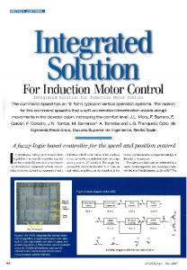
Fig. 4. Rotor resistance variation (Rr )
Fig. 1. Tracking performance ω (k) (solid line), x1 (k) (dash-dot line) and ω r (k) (dashed line).
100 90 80
0.6
70 60 ||wi||
0.5
0.4
50
wb2
40
0.3
30 20
0.2
w54
w44
10
0.1
0
0
0
500
1000
1500
2000 t(ms)
2500
3000
3500
0
500
1000
1500
2000 t(ms)
2500
3000
3500
4000
3500
4000
4000
Fig. 5. Weight evolution Fig. 2. Tracking performance Ψ (k) (solid line), line) and Ψd (k) (dashed line).
x22 +x23
(dash-dot 1 0.8
2.5
0.6 2
0.4
Tl (Nm)
1.5
0.2 0
1
-0.2
0.5
-0.4 0
-0.6 -0.5
0
100
200
300
400
500 t(ms)
600
700
Fig. 3. Load torque TL (k)
800
900
0
500
1000
1500
2000
2500
3000
1000
Fig. 6. Time evolution of ψ α (k) and its estimate (real in solid line and estimated in dashed line)
8
discrete-time recurrent neural networks with stable learning algorithms”, Information Sciences, Vol. 158, pp. 131-147, 2004.
1 0.8 0.6 0.4 0.2 0 -0.2 -0.4 -0.6
0
500
1000
1500
2000
2500
3000
3500
4000
Fig. 7. Time evolution of ψ β (k) and its estimate (real in solid line and estimated in dashed line)
References [1] [2] [3]
[4] [5] [6] [7] [8] [9] [10]
[11] [12] [13]
[14]
[15] [16]
C. K. Chui and G. Chen, Kalman Filtering with Real-Time Applications, 3rd ed., Springer-Verlag, New York, USA, 1998. R. A. Felix, E. N. Sanchez and A.G. Loukianov, “Avoding controller singularities in adaptive recurrent neural control”, Proceedings IFAC’05, Praga, July, 2005. S. S. Ge, J. Zhang and T.H. Lee,“Adaptive neural network control for a class of MIMO nonlinear systems with disturbances in discrete-time”, IEEE Transactions on Systems, Man and Cybernetics, Part B, Vol. 34, No. 4, August, 2004. R. Grover and P. Y. C. Hwang, Introduction to Random Signals and Applied Kalman Filtering, 2nd ed., John Wiley and Sons, New York, USA, 1992. H. Khalil, Nonlinear Systems, 2nd ed, Prentice Hall, Upper Saddle River, N. J., USA, 1996. F. Khorrami, P. Krishnamurthy and H. Melkote, Modeling and Adaptive Nonlinear Control of Electric Motors , Springer-Verlag, New York, USA, 2003. Leonard W. (1986), “Microcomputer control of high dynamic performance AC-drives- a survey”, Automatica, Vol.22, pp. 1-19. A. G. Loukianov, J. Rivera and J. M. Cañedo, “Discretetime sliding mode control of an induction motor”, Proceedings IFAC’02, Barcelone, Spain, July, 2002. Luca A. D. and G. Ulivi. (1989). “Design of exact nonlinear controller for induction motors”, IEEE Trans. Automat. Control, Vol.34, pp. 1304-13 E. N. Sanchez, A. Y. Alanis and G. Chen, “Recurrent neural networks trained with Kalman filtering for discrete chaos reconstruction”, Proceedings of Asian-Pacific Workshop on Chaos Control and Synchronization’04, Melbourne, Australia, July, 2004. G. A. Rovithakis and M. A. Chistodoulou, Adaptive Control with Recurrent High -Order Neural Networks, Springer Verlag, New York, USA, 2000. Shabanovic A. and D. Izosimov. (1981) “Application of sliding modes to induction motor control”, IEEE Trans.Ind.Applicat., Vol. 17, pp. 41-49. S. Singhal and L. Wu, Training multilayer perceptrons with the extended Kalman algorithm, in D. S. Touretzky (ed), Advances in Neural Information Processing Systems 1, pp. 133140, Morgan Kaufmann, San Mateo, CA, USA, 1989. Y. Song and J. W. Grizzle, "The extended Kalman filter as local asymptotic observer for discrete-time nonlinear systems", Journal of Mathematical systems, Estimation and Control,Vol. 5, No. 1, pp. 59-78, Birkhauser-Boston, 1995. Utkin V. A. (1993). “AC drives control problems”, Avtomatica i Telemekhanika, No. 12, pp. 53-65. W. Yu and X. Li, “Nonlinear system identification using