MULTIVARIABLE ADAPTIVE CONTROL USING A RECURRENT NEURAL NETWORK HENRIQUES, J. and DOURADO, A. CISUC - Centro de Informática e Sistemas da Universidade de Coimbra Departamento de Engenharia Informática - Universidade de Coimbra - Pinhal de Marrocos, 3030 Coimbra, Portugal
[email protected],
[email protected]
Abstract An indirect adaptive controller based on a hybrid solution is presented and applied. Using data concerning the process, a dynamic recurrent neural network (Elman’s type) is trained to model a general nonlinear discrete time system. By assuming a linearisation of this neural model, a time varying standard linear state space model is derived. As a consequence, some well-established conventional technique for linear systems can be applied. With simultaneous online training of the neural network and controller synthesis, the resulting algorithm is adaptive. In order to evaluate its performance, the developed methodology is applied to a multivariable real process, a three tanks laboratory system. For this particular process the experimental results shows the effectiveness of the proposed methodology.
Keywords: Recurrent neural networks, Multivariable Adaptive Nonlinear Control, Decoupling
1. Introduction The use of linear conventional control theory applied to real plants, generally nonlinear and multivariable, leads in many cases to suboptimal performances. Also, due to uncertainty in the knowledge, it is not easy to derive a linear model that describes the system properly. In last years, the application of neural networks (NN) for adaptive control has been a subject of extensive study. In this field several works have been presented. Narendra [1] has introduced the idea that a more general flexible control law could be provided using the nonlinear function approximation property of NN. Chen [2] proposed a scheme for combining backpropagation neural networks with selftuning adaptive control and [3] presented an analytical study of the use of multilayer neural networks in the control of the affine class of nonlinear discrete time systems. Jin [4] proposed an adaptive scheme for a general class of unknown nonlinear multivariable discrete time systems and Delgado [5] proposed a generalisation of the Hopfield’s NN to identify and control the affine class of control systems. Among the NN, the dynamic recurrent neural network (DRNN), which involves dynamic elements and have feedback connections, are considered more suitable for dynamical systems. It has been shown, Jin [6], that a discrete time DRNN may be used to approximate, with an arbitrary precision, a discrete time state space representation which is produced from either a discrete time system or a continuos function. In this paper, a strategy that combines the DRNN model with selftuning indirect adaptive control, is proposed. The architecture of the DRNN mimics, in some sense, the block diagram of linear state space equation but with nonlinear blocks. The proposed control structure is based on the DRNN model linearisation at every operating point. A standard linear state space model of the form x ( k +1) = Ax ( k ) + Bu( k ) is derived and a state space feedback controller u ( k ) = Fx ( k ) + Gr ( k ) , combining simultaneously decoupling and pole placement design is applied. With simultaneous online training of the DRNN and control synthesis the resulting algorithm is an indirect adaptive control law. This methodology is applied to the nonlinear multivariable three tanks system DTS200 [7]. The experimental results show the effectiveness of the proposed hybrid approach with respect to set-point tracking. 2. Process Modelling with DRNN We assume that the dynamical system to be controlled is described by the nonlinear discrete state equation
p
q
X ( k ) = f [ X ( k −1), U ( k −1) ]
(1a)
Y ( k )= C X (k )
(b)
n
where U ( k )∈ℜ , Y ( k )∈ℜ and X ( k )∈ℜ and they represent the input, output and state vectors respectively at discrete time k. f is a nonlinear function and C a (q,n) matrix. We also assume that all the states are accessible.
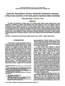
2.1 - Elman´s Network In this paper an Elman’s network [8] is used to approximate the nonlinear function f, using the available data concerning the system. In addition to the input U(k), output Y(k) and hidden units X$ ( k ) , an Elman’s network has a context unit X c ( k ) . The interconnection
Input Units
Hidden Units
^ Y(k) X(k) U(k-1) matrices are W xu ∈ℜ n , p , W xc ∈ℜ n ,n and W yx ∈ℜ q ,n , 1 1 .1 .1 .1 xu yx . . . respectively for the context-hidden layer, input-hidden W W . . . U(k-1) p Y(k) q layer and hidden-output layer, as shown in figure 1. p q n Theoretically an Elman’s network is able to represent an Output xc Units W nth order dynamic system if it has n hidden units. α . 1 . . However, due to practical difficulties with the c n X (k) identification of higher order systems, selfconnections (αα Context Units fixed value, not modified by training) in the context units Figure 1 - Elman’s Dynamic Recurrent Network can be introduced improving the dynamic memorisation ability of the network [8]. The context units are used to memorise the previous information of the hidden units and can be viewed as a one step time delay. The feedforward connections are modifiable and the recurrent connections are fixed. The dynamics of the neural network is described by the following difference equation
[
X$ ( k )=σ W xc X c ( k ), W xuU ( k −1)
]
X c ( k ) =αX c ( k −1) + X$ ( k −1) Y ( k ) =W
yx
(2a) (b)
X$ ( k )
(c)
where σ{.} is a nonlinear function (usually a sigmoidal type). 2.2 - Learning methodology There are several training algorithms that have been proposed for adjust the DRRN weights. Examples of these methods are the Narendra’s dynamic backpropagation, the real time recurrent algorithm from Williams and the Werbos’ backpropagation trough time (BTT) [9], which is used in this work. Due to the computational complexity of the BTT, a natural simplification is obtained by truncating the backpropagation of information to a fixed number (N) of prior time steps on a sliding window mode. The network is duplicated N times in order to describe the behaviour on the considered time window, and standard backpropagation algorithm can be applied through the global static network. In this work N=4, establishing a compromise between computational complexity and system order representation. The performance criterion to be minimised is defined as: J total [ k − N ,k ]=
k
∑
(3)
e( k ) 2
τ =k − N
where k is the actual instant and e( k ) = X ( k ) − X$ ( k ) . The computation of the gradient of J total is obtained after the NN has been run through the interval [k-N…k]. Then the values ε(τ) and δ(τ), for τ∈[k-N…k], are computed recursively using the following equations
[
ε L (τ ) = e L (τ )
(4a)
]
δ L (τ ) = σ ′ W X (k ), W U (k − 1) ε L (τ )
(b)
ε L (τ −1) =e L (τ −1) +∑Wiτ δ L (τ )
(c)
xc
c
xu
i
These equations represent the well known backpropagation in which target values are specified for units in all layers (L) and not only in the last layer (in the standard BP e L (τ −1)= 0 , equation 4c). The total gradient is k ∂ J total [k − n, k ] = ∑ δ i (τ )Xˆ j (τ − 1) ∂ Wij τ = k − N +1
(5)
2.3 – Linearisation the Neural Model σ{.} is a nonlinear function. However it is possible to derive a linear model by computing the derivatives from the outputs with respect to the inputs of the network. In this topic there has been some works: Ahmed [10] proposed a control scheme based on plant linearisation at each operating point. Following this author, since control design for linear systems has been well developed, it is natural to make use of it in nonlinear plants. Sørenson [11] has shown the possibility to extract online, from a nonparametric neural model, the actual linearised parameters. Using the features of this strategy for parameter estimation, a conventional pole
placement adaptive controller can be adopted for nonlinear control. In fact, using equation 2a), a standard space state model can be obtained by taking the derivatives of the outputs with respect to the inputs X$ ( k ) = AX$ ( k −1) + BU ( k −1)
(6)
Yˆ (k ) = CXˆ ( k ) where the (n,n) A matrix, the (n,m) B and the (m,n) C matrices are defined by A=
∂ σ{ } =W xcσ ′{ ∂ X$ ( k −1)
}
B=
∂ σ{
}
∂ U ( k −1)
=W xu σ ′{
}
(b)
C = W yx
(7)
3. Decoupling Pole Placement Control Design The prior information concerning the system determines how the control problem must be formulated as well as what method should be used for its solution. In this work we assume that all the states X (k ) are acessible and the number of inputs is equal to the number of outputs (m=p=q). Also, following section 2, there exist a time varying dynamic system that describes in each instant the nonlinear multivariable plant. Then we have a nonlinear multivariable adaptive control problem. Assuming the system described by equation (6), a state feedback control law is defined by U ( k ) = FX ( k ) +GR ( k )
(8)
q
where R( k )∈ℜ is the setpoint vector. F and G are respectively (m,n) and (m,m) matrices computed by a pole placement law and such that the i th input Ri ( k ) affects only the i th output Yi ( k ) .Falb [12] has established this decoupling pole placement control law. Let d 1 ,Ld m
{
}
d i =min j: Ci A j B≠0 or d i =n−1 if Ci A j B=0
(9)
Then the F and G matrices are defined by −1 λ F = B * ∑ M l CA l − A* l =0
G = B *−1
(10)
where C1 A d 1 B B*= M C A dm B m
C1 A d 1+1 A*= M C A dm+1 m
(11)
λ=max{d i } and the M l matrices are suitably chosen to specify the close loop pole location.
4. Experimental Results 4.1 - The Three Tank System - DTS200 The DTS200 three tank system [7] is a nonlinear system which consists of three plexiglas interconnected in series by two connecting pipes (see figure 2). The liquid leaving T2 is collected in a reservoir from which pumps 1 u1 u2 Pump 1 Pump2 and 2 supply the tanks T1 and T2. The three tanks are h1 h3 equipped with piezo-resistive pressure transducer for h2 measuring the level of the liquid (usually distilled water). T1 T3 T2 A digital controller controls the flow rate u1 and u2 such that the levels in the tanks T1 and T2 can be set independently. The connecting pipes and the tanks are additionally equipped with manually adjustable valves and NO - Normally Open NC - Normally Closed outlets for the purpose of simulating clogs as well as leaks. Figure 2 - A schematic diagram of the DTS200 There are three measurable state variables, h1, h2 and h3. The goal of the control system is to control the level h1 and h2 by adjusting the flow rate u1 and u2. NO
NC
NO
NC
NO
NC
4.2 - The adaptive DRNN model / Decoupling Pole Placement Controller For control purposes we assume the system described by equation (6) with m=2 and n=3. Also, for this particular system, C is fixed and define as C = [1 0 0; 0 1 0]. F and G are computed with the goal that the pump flow u1 affects only the level h1 and the pump flow u2 affects only the level tank h2. In the experiments, the pole location were chosen to be equal for both subsystems (p1=p2=0.9). A priori knowledge about the process was assumed in form of a linear state space equation that was used to initialise the weights of the DRNN. For
the learning stage a learning rate equal to 0.02 was chosen. The sampling time is 1 second and the input/output variables (u1, u2, h1, h2 and h3) were scaled to the range [0…1]. 4.3 - Experiments Figure 3 shows the behaviour of the controller with respect to setpoint tracking. As can be seen the controller performed considerably well and the decoupling characteristic can be clearly observed. 1
0.4 0.35
u1
0.8 r1
0.3
h1
0.6
h3
0.25 0.4
r2
0.2 h2
0.2
0.15 0.1
0
1
2
3
4
5
6
7
8
0 0
u2
1
Time -Minutes
2
3
4
5
6
7
8
Time -Minutes
Figure 3 - Set-Point Tracking
5. CONCLUSIONS In this paper it was developed and applied a strategy of applying DRNN in an indirect adaptive scheme with a conventional linear controller. The ability of an Elman’s DRNN, with online learning, was used to the identification of an arbitrary dynamic nonlinear system and a conventional decoupling pole placement technique was used to derive the adaptive control law. The effectiveness of this strategy was validated in a multivariable real process, the DTS200. In this work no efforts have been made to establish theoretical probes about stability of the closed loop. This problem and the applicability of the methodology to differents systems will be investigated in future research. It is believed that NN can be effectively used for control design of nonlinear systems and they must be seen as an extension to the conventional techniques rather than a replacement. Acknowledges: this work was partially financed by JNICT/PRAXIS XXI.
REFERENCES [1] Narendra K., Parthasarathy K. (1990) - Identification and control of dynamical systems using neural networks IEEE Trans. Neural Networks, Vol 1, pp 4-27 [2] Chen, F-C (1990) - Back propagation neural networks for nonlinear self-tuning adaptive control IEEE Control System Magazine, Special Issue on Neural Networks for control - pp 45-48 [3] Chen, F-C (1995) - Adaptive control of a class of nonlinear discrete-time systems using neural networksIEEE Trans. Automatic Control, Vol 40, nº 7, pp 791-801 [4] Jin L. et al (1994) - Adaptive control of discrete time nonlinear system using recurrent neural networks IEE Proc. Control Theory Applications, Vol 141, nº 3 [5] Delgado, A. et al (1995) - Dynamic recurrent neural networks for system identification and control IEE Proc. Control Theory Applications, Vol 142, nº 4, pp 307-314 [6] Jin L. et al (1995) - Approximation of discrete time state space trajectories using dynamic recurrent networks IEEE Trans. Automatic Control, Vol 40, nº 7, pp1266-1270 [7] Three Tank System DTS200 (1996) -Laboratory Setup - Amira GmbH [8] Pham D, Xing, L. (1995) - Dynamic System Identification Using Elman and Jordan Networks Neural Networks for Chemical Engineers, Editor A. Bulsari, Chap. 23, pp 572-591 [9] Werbos P (1990) - Backpropagation trough time: what it does and how do it- Proc IEEE, 78, 1550-1560 [10] Ahmed M, (1994) - Neural net controller for nonlinear plants: design approach trough linearisation IEE Proc. Control Theory Applications, Vol 141, nº5, pp315-322 [11] Sørensen O. (1996) - Nonlinear pole placement control with a neural network - EJC, Vol 2, pp 36-43 [12] Falb P Wolovith, (1967) - Decoupling in the Design and Synthesis of Multivariable Control Systems IEEE Trans. Automatic Control, Vol 12, nº 6, pp 651-659