Fast Shortest Path Distance Estimation in Large Networks Michalis Potamias1∗ Francesco Bonchi2 Carlos Castillo2 Aristides Gionis2 1
Computer Science Department Boston University, USA
[email protected]
ABSTRACT In this paper we study approximate landmark-based methods for point-to-point distance estimation in very large networks. These methods involve selecting a subset of nodes as landmarks and computing offline the distances from each node in the graph to those landmarks. At runtime, when the distance between a pair of nodes is needed, it can be estimated quickly by combining the precomputed distances. We prove that selecting the optimal set of landmarks is an NP-hard problem, and thus heuristic solutions need to be employed. We therefore explore theoretical insights to devise a variety of simple methods that scale well in very large networks. The efficiency of the suggested techniques is tested experimentally using five real-world graphs having millions of edges. While theoretical bounds support the claim that random landmarks work well in practice, our extensive experimentation shows that smart landmark selection can yield dramatically more accurate results: for a given target accuracy, our methods require as much as 250 times less space than selecting landmarks at random. In addition, we demonstrate that at a very small accuracy loss our techniques are several orders of magnitude faster than the state-of-the-art exact methods. Finally, we study an application of our methods to the task of social search in large graphs. Categories and Subject Descriptors H.4.3 [Information Systems Applications]: Communications Applications General Terms Algorithms Keywords Graphs, shortest-paths, landmarks methods.
1. INTRODUCTION Understanding the mechanisms underlying the characteristics and the evolution of complex networks is an important task, which has received interest by various disciplines ∗
Part of this work was done while the first author was visiting Yahoo! Research Barcelona, under the Yahoo! internship program.
Permission to make digital or hard copies of all or part of this work for personal or classroom use is granted without fee provided that copies are not made or distributed for profit or commercial advantage and that copies bear this notice and the full citation on the first page. To copy otherwise, to republish, to post on servers or to redistribute to lists, requires prior specific permission and/or a fee. CIKM’09, November 2–6, 2009, Hong Kong, China. Copyright 2009 ACM 978-1-60558-512-3/09/11 ...$10.00.
Yahoo! Research Barcelona, Spain
2
{bonchi,chato,gionis}@yahoo-inc.com
including sociology, biology, and physics. In the last years we have witnessed a continuously increasing availability of very large networks; blogs, sites with user-generated content, social networks, and instant messaging systems nowadays count hundreds of millions of users that are active on a daily basis. For graphs of this size, even seemingly simple algorithmic problems become challenging tasks. One basic operation in networks is to measure how close one node is to another, and one intuitive network distance is the geodesic distance or shortest-path distance. Computing shortest-path distances among nodes in a graph is an important primitive in a variety of applications including, among many others, social-network analysis, VLSI design in electronics, protein interaction networks in biology and route computation in transportation. Recently, new motivating applications have arisen in the context of web search and social networks. In web search, the distance of a query’s initiation point (the query context) to the relevant web-pages could be an important aspect in the ranking of the results [34]. In social networks, a user may be interested in finding other users, or in finding content from users that are close to her in the social graph [30]. This socially sensitive search model has been suggested as part of the social network search experience [2, 36]. Using the shortest path distance as a primitive in ranking functions for search tasks is the main motivation of our work. Although computing shortest paths is a well studied problem, exact algorithms can not be adopted for nowadays real-world massive networks, especially in online applications where the distance must be provided in the order of a few milliseconds. A full breadth-first search (BFS) traversal of a web-graph of 4 M nodes and 50 M edges takes roughly a minute in a standard modern desktop computer.1 For the same graph the best known point-to-point shortest path algorithms that combine Dijkstra with A* and landmarks, require to access an average of 20 K nodes in order to determine the shortest path between two nodes. On the other hand, precomputing all the shortest paths and storing them explicitly is infeasible: one would need to store a matrix of approximately 12 trillion elements. The methods described in this paper use precomputed information to provide fast estimates of the actual distance in very short time. The offline step consists of choosing a subset of nodes as landmarks (or reference objects) and computing distances from every node to them. Such precomputed distance information is often referred to as an embedding. Our contribution. In this paper we present an extensive analysis of various strategies for selecting landmarks. We 1
Using the BFS routine of C++ Boost library.
devise and experimentally compare more than 30 strategies that scale well to very large networks. For presentation sake, we report the best ones; in case of ties we report the simplest. Our experimentation shows that for a given target accuracy, our techniques require orders of magnitude less space than random landmark selection, allowing an efficient approximate computation of shortest path distances among nodes in very large graphs. To the best of our knowledge, this is the first systematic analysis of scalable landmarks selection strategies for shortest-path computation in large networks. Our main contributions are summarized as follows: • We define the problem of optimal landmark selection in a graph and prove that it is NP-hard (Section 3). • We theoretically motivate and suggest simple and intuitive strategies to choose landmarks that scale well to huge graphs (Section 4). • We demonstrate the effectiveness and robustness of our techniques experimentally using five large different real-world networks with millions of edges (Section 5). • We report significant efficiency gains with respect to the state-of-the-art. We study the triangulation performance of landmark selection methods (Section 5.4). Although theoretical bounds have been proven in literature [24] for random landmarks selection we prove empirically that our methods outperform it by large margins on real networks. With respect to exact algorithms we show that several orders of magnitude in efficiency can be traded-off with a very small loss in accuracy using the proposed techniques (Section 5.5). • We apply our methods to social search (Section 6), showing high precision and accuracy in the problem of finding the closest nodes in the graph that match a given query. In our experimental evaluation we use real world networks: social graphs with explicit or implicit links from Flickr, a graph based on the communication network of the Yahoo! Instant Messenger service, and the coauthorship graph from the DBLP records. We also use a web-graph defined by the Wikipedia pages and their hyperlinks. Paper structure. In Section 2 we outline the related work, and in Section 3 we introduce our notation and our algorithmic framework. Section 4 presents a series of landmark section strategies which are experimentally evaluated in Section 5. Section 6 evaluates an application of our methods for fast social-network-aware search. Finally, Section 7 presents some concluding remarks.
2. RELATED WORK Exact shortest-path distances. Dijkstra described the algorithm to compute single source shortest paths (SSSP) in weighted graphs with n nodes and m edges from a node to all others [11]. The cost is O(n2 ) in general and can be reduced to O(m + n log n) for sparse graphs. For unweighted graphs, shortest paths can be computed using Breadth First Search (BFS) in time O(m + n). Floyd-Warshall algorithm employs dynamic programming to solve the all-pairs shortest paths (APSP) problem in an elegant and intuitive way [13] in time O(n3 ). Still, the complexity of computing APSP by invoking
n Dijkstra/BFS computations is asymptotically faster, since it costs O(nm + n2 log n) and O(nm) respectively. The state of the art in point to point shortest path (PPSP) queries involves combining bidirectional Dijkstra with A* and lower bounds (ALT algorithms) [16, 17, 37, 27, 22]. ALT algorithms employ landmarks in order to prune the search space of the shortest path computation. Their landmarks are similar to the ones we experimented with for the lower-bound estimation (see Section 4.4); instead, in this paper, we use heuristics for selecting landmarks that work well with upper-bound estimates. Our paper addresses a different problem than the one in [16, 17, 37, 27, 22] since we are interested only on the length of a shortest path, not the path itself. Thus, we avoid any kind of online Dijkstra/BFS traversals of the graph. However, to demonstrate the savings that one can obtain if the path itself is not of interest, and if only the distance length between two nodes is important, in Section 5 we compare our method to these state-of-the-art techniques and demonstrate that orders of magnitude in efficiency can be gained with a very small loss in accuracy. Indexing for approximate shortest-paths. We are interested in preprocessing a graph so that PPSP queries can be answered approximately and quickly at runtime. Thorup and Zwick [32] observe that this problem is probably the most natural formulation of the APSP. In their paper they obtain the result that for any integer k ≥ 1 a graph can be 1 preprocessed in O(kmn k ) expected time, using a data struc1 ture of size O(kn1+ k ), and a PPSP query can be processed in time O(k). The quotient of the division of the estimated distance and the exact is guaranteed to lie within [1, 2k − 1]. For k = 1 we get the exact solution of computing all shortest paths and storing them, which is prohibitively expensive. For k = 2 the estimate may be three times larger than the actual distance. In large real-world graphs this bound is already problematic because distances are short due to the small-world phenomenon. In a small-world network, such as the Flickr-contacts graph described in Section 5, for an estimated distance of 6, the exact distance is only guaranteed to lie within the interval [2, 6], along with almost every pairwise distance in this graph. A survey on exact and approximate distances in graphs can be found in [38]. Embedding methods. Our work is related to general embedding methods. In domains with a computationally expensive distance function, significant speed-ups can be obtained by embedding objects into another space and using a more efficient distance function, such as an Lp norm. Several methods have been proposed to embed a space into a Euclidean space [6, 20]. There have been attempts to optimize the selection of reference objects for such a setting [3, 35]. Other dimensionality reduction techniques are also widely studied especially in theory and machine learning. Landmarks have already been used for graph measurements in many applications [10, 26, 31, 28] such as roundtrip propagation and transmission delay in networks: however, how to optimally select the location of landmarks has not been extensively studied. Kleinberg et al. [24] discuss the problem of approximating network distances in real networks via embeddings using a small set of beacons (i.e., landmarks). Of most interest is the fact that they introduce in their analysis the notion of slack, as a fraction of pairs in the network for which the
algorithm provides no guarantees. Their analysis considers choosing beacons randomly. In this paper we show that in practice, simple intuitive strategies work much better than the random. Abraham et al. [1] generalize the metric embedding with slack. On another perspective, computing shortest paths in spatial networks has also attracted interest recently [25, 29]; our work is different since we focus on graphs that exhibit complex social network or web-graph behavior. Applications. Our work is also tightly connected to the various notions that have been introduced to measure the centrality of a vertex. Betweenness centrality measures the amount of shortest paths passing from a vertex while closeness centrality measures the average distance of a vertex to all other vertices in the network [15]. Brandes [7] gave the best known algorithm to compute the exact betweenness centrality of all vertices by adapting the APSP Dijkstra algorithm. The algorithm runs in O(nm+n2 logn) time, which is prohibitive for large graphs. Bader et al. [4] gave a sampling-based approximation algorithm and showed that centrality is easier to approximate for central nodes. In our work, we use closeness centrality as a strategy in choosing central points as landmarks in the graph. Fast PPSP computation is becoming very relevant for Information Retrieval. Socially sensitive search in social networks and location-aware search are attracting a substantial interest in the information retrieval community [5]. For instance, it has been found that people who chat with each other are more likely to share interests [30]. An experiment discussed in Section 5 considers ranking search results in social networks based on shortest path distances. This problem has also been studied recently by Vieira et al. [36]. Their work is also based on landmarks, but their landmarks are chosen randomly. Since our work has been inspired by the task of social search we revisit it in Section 6 and show that our techniques outperform the random landmark selection [36] by very large margins. Approximation methods for computing other graph proximity functions that are based on random walks, such as personalized pagerank and random walk with restart, have also been studied recently [14, 33]. The growing interest in involving context and/or social connections in search tasks, suggests that distance computation will soon be a primitive of ranking functions. The restriction is that the ranking functions of search engines have hard computational deadlines to meet, in the order of hundreds of milliseconds. Our methods can provide accurate results within these deadlines.
3. ALGORITHMIC FRAMEWORK In this section we introduce the notation that we use in the rest of the paper. We then describe how to index distances very efficiently using landmarks. We formally define the landmark-selection problem that we consider in this paper, and prove that it is an NP-hard problem.
3.1 Notation Consider a graph G(V, E) with n vertices and m edges. Given two vertices s, t ∈ V , define πs,t = hs, u1 , u2 , ..., uℓ−1 , ti to be a path of length |πs,t | = ℓ between s and t, if {u1 , ..., uℓ } ⊆ V and {(s, u1 ), (u1 , u2 ), . . . , (uℓ−1 , t)} ⊆ E, and let Πs,t be the set of all paths from s to t. Accordingly, let dG (s, t) be the length of the shortest path between any two vertices s, t ∈ V , we refer to this as the geodesic distance, or distance, between such vertices. In other words, dG (s, t) =
u
s
t u
s
t
Figure 1: Illustration of the cases for obtaining tight upper bounds (left) and tight lower bounds (right) as provided by Observations 1 and 2 ∗ |πs,t | ≤ |πs,t | for all paths πs,t ∈ Πs,t . Let SPs,t be the set of paths whose length is equal to dG (s, t). For simplicity we consider unweighted, undirected graphs, but all the ideas in our paper can be easily applied to weighted and/or directed graphs. Consider an ordered set of d vertices D = hu1 , u2 , . . . , ud i of the graph G, which we call landmarks. The main idea is to represent each other vertex in the graph as a vector of shortest path distances to the set of landmarks. This is also called an embedding of the graph. In particular, each vertex v ∈ V is represented as a d-dimensional vector φ(v):
φ(v) = hdG (v, u1 ), dG (v, u2 ), ..., dG (v, ud )i
(1)
For ease of presentation, from now on we will denote the i-th coordinate of φ(v) by vi , i.e., vi = dG (v, ui ).
3.2
Distance bounds
The shortest-path distance in graphs is a metric, and therefore it satisfies the triangle inequality. That is, given any three nodes s, u, and t, the following inequalities hold. dG (s, t) ≤ dG (s, u) + dG (u, t), dG (s, t) ≥ |dG (s, u) − dG (u, t)|
(2) (3)
An important observation that we will use to formulate the landmark-selection problem is that if u belongs to one of the shortest paths from s to t, then the inequality (2) holds with equality. Observation 1. Let s, t, u be vertices of G. If there exists a path πs,t ∈ SPs,t so that u ∈ πs,t then dG (s, t) = dG (s, u) + dG (u, t). A similar condition exists for the inequality (3) to be tight, but in this case, it is required that either s or t are the “middle” nodes. Observation 2. Let s, t, u be vertices of G. If there exists a path πs,u ∈ SPs,u so that t ∈ πs,u , or there exists a path πt,u ∈ SPt,u so that s ∈ πt,u , then dG (s, t) = |dG (s, u) − dG (u, t)|. The situation described in Observations 1 and 2 is shown in Figure 1.
3.3
Using landmarks
Given a graph G with n vertices and m edges, and a set of d landmarks D, we precompute the distances between each vertex in G and each landmark. The cost of this offline computation is d BFS traversals of the graph: O(md). Recall that our task is to compute dG (s, t) for any two vertices s, t ∈ V . Due to Inequalities (2) and (3), we have max |si − ti | ≤ dG (s, t) ≤ min{sj + tj }. i
j
In other words, the true distance dG (s, t) lies in the range [L, U ], where L = maxi |ti − si | and U = minj {sj + tj }.
Notice that one landmark may provide the best lower bound and another the best upper bound. Any value in the range ˜ t) for the real value of [L, U ] can be used as an estimate d(s, dG (s, t). Some choices include using the upper bound d˜u (s, t) = U, using the lower bound d˜l (s, t) = L,
cost O(nm) for unweighted graphs and O(nm + n2 log n) for weighted graphs. Additionally, Bader et al. [4] discuss how to approximate betweenness centrality by random sampling. For our problem, consider a modified definition of betweenness centrality according to which we define Ist (u) to be 1 if u lies on at least one shortest path from s to t, and 0 otherwise. We then define X Ist (u). (5) C(u) = s6=u6=t∈V
the middle point L+U , d˜m (s, t) = 2 or the geometric mean √ d˜g (s, t) = L · U . Notice that in all cases the estimation is very fast, as only O(d) operations need to be performed, and d can be thought of as being a constant, or a logarithmic function of the size of the graph. Our experiments indicate that the “upper bound” estimates d˜u (s, t) = U work much better than the other types of estimates, so, in the rest of the paper, we focus on the upper-bound estimates. We only comment briefly on lowerbound estimates later in Section 4.4. As follows by Observation 1, the approximation d˜u (s, t) is exact if there exists a landmark in D, which is also in a shortest path from s to t. This motivates the definition of coverage: Definition 1. We say that a set of landmarks D covers a specific pair of vertices (s, t) if there exists at least one landmark in D that lies in one shortest path from s to t. Our landmark-selection problem is formulated as follows. Problem 1 (landmarksd ). Given a graph G = (V, E) select a set of d landmarks D ⊆ V so that the number of pairs of vertices (s, t) ∈ V × V covered by D is maximized. A related problem is the following Problem 2 (landmarks-cover). Given a graph G = (V, E) select the minimum number of landmarks D ⊆ V so that all pairs of vertices (s, t) ∈ V × V are covered.
3.4 Selecting good landmarks To obtain some intuition about landmark selection, consider the landmarksd problem for d = 1. The best landmark to select, is a vertex that it is very central in the graph, and many shortest paths pass through it. In fact, selecting the best landmark is related to finding the vertex with the highest betweenness centrality [15]. To remind the reader the definition of betweenness centrality, given two vertices s and t, let σst denote the number of shortest paths from s to t. Also let σst (u) denote the number of shortest paths from s to t that some u ∈ V lies on. The betweenness centrality of the vertex u is defined as X σst (u) (4) CB (u) = σst s6=u6=t∈V
The fastest known algorithms to compute betweenness centrality exactly are described by Brandes [7]. They extend well-known all-pairs-shortest-paths algorithms [9]. The time
It follows immediately that the optimal landmark for the landmarksd problem with d = 1 is the vertex that maximizes C(u). Our modified version C(u) can be computed as efficiently as CB (u) by modifying Brandes’ algorithm [7].
3.5
Problem complexity and approximation algorithms
Both of the problems landmarksd and landmarks-cover are NP-hard. An easy reduction for the landmarks-cover problem can be obtained from the vertex-cover problem. Theorem 1. landmarks-cover is NP-hard. Proof. We consider the decision version of the problems landmarks-cover and vertex-cover. The latter problem is defined as follows: given a graph G, and an integer k, decide if there is a subset of vertices V ′ ⊆ V of size at most k so that for all edges (u, v) ∈ E either u ∈ V ′ or v ∈ V ′ . Transform an instance of vertex-cover to an instance of landmarks-cover. Consider a solution D for landmarkscover. Consider now the set of all 1-hop neighbors and observe that each pair is connected by a unique shortest path of length 1 (i.e. an edge). Since all pairs of vertices are covered, so are 1-hop neighbors, therefore the edges of E are also covered by D, therefore, D is a solution to vertex-cover. Conversely, consider a solution V ′ for vertex-cover. Consider a pair of vertices (s, t) ∈ V × V , and any shortest path πs,t between them. Some vertices of V ′ should be on the edges of the path πs,t , and therefore V ′ is also a solution to landmarks-cover. As a consequence, landmarksd is also NP-hard. Next we describe a polynomial-time approximation solution to the landmark-selection problem. The main idea is to map the problem to set-cover problem. Given the graph G = (V, E), we consider a set of elements U = V × V and a collection of sets S, so that each set Sv ∈ S corresponds to a vertex v ∈ V . A set Sv contains an element (s, t) ∈ U if v lies on a shortest path from s to v. Thus, solving the set-cover problem on (U, S) with the greedy algorithm [8], we obtain a O(log n)-approximation to landmarks-cover problem and a (1 − 1/e)-approximation to landmarksd problem. However, the running time of the above approximation algorithm is O(n3 ), which is unacceptable for the size of graphs that we consider in this paper. The suggested strategies of the next section are motivated by the observations made in this section regarding properties of good landmarks.
4.
LANDMARK-SELECTION STRATEGIES
This section describes our landmark-selection strategies. The baseline scalable strategy is to select landmarks at random [36, 24, 31]. The strategies we propose are motivated by the discussion in the previous section. On a high
level, the idea is to select as landmarks “central” nodes of the graph, so that many shortest paths are passing through. We use two proxies for selecting central nodes: (i) high-degree nodes and (ii) nodes with low closeness centrality, where the closeness Pcentrality of a node u is defined as the average distance n1 v dG (u, v) of u to other nodes in the graph. In order to cover many different pairs of nodes, we need to spread the landmarks throughout the graph. In accordance, we propose two improvements for our strategies: (i) a constrained variant, where we do not select landmarks that are too close to each other, and (ii) a partitioning variant, where we first partition the graph and then select landmarks from different partitions.
4.1 Basic strategies Random: The baseline landmark-selection strategy consists of sampling a set of d nodes uniformly at random from the graph. Degree: We sort the nodes of the graph by decreasing degree and we choose the top d nodes. Intuitively, the more connected a node is, the higher the chance that it participates in many shortest paths. Centrality: We select as landmarks the d nodes with the lowest closeness centrality. The intuition is that the closer a node appears to the rest of the nodes the bigger the chance that it is part of many shortest paths. Computing the closeness centrality for all nodes in a graph is an expensive task, so in order to make this strategy scalable to very large graphs, we resort to computing centralities approximately. Our approximation works by selecting a sample of random seed nodes, performing a BFS computation from each of those seed nodes, and recording the distance of each node to the seed nodes. Since the seeds are selected uniformly at random and assuming that graph distances are bounded by a small number (which is true since real graphs typically have small diameter), we can use the Hoeffding inequality [21] to show that we can obtain arbitrarily good approximation to centrality by sampling a constant number of seeds.
4.2 Constrained strategies Our goal is to cover as many pairs as possible. Using a basic strategy such as the ones described above, it may occur that the second landmark we choose covers a set of pairs that is similar to the one covered by the first, and thus its contribution to the cover is small. The constrained variant of our strategies depends on a depth parameter h. We first rank the nodes according to some strategy (e.g., highest degree or lowest closeness centrality). We then select landmarks iteratively according to their rank. For each landmark l selected, we discard from consideration all nodes that are at distance h or less from l. The process is repeated until we select d landmarks. We denote our modified strategies by Degree/h and Centrality/h. For the experiments reported in the next section we use h = 1, 2, 3 and we obtain the best results for h = 1. So, in the rest of the paper, we only consider this latter case.
4.3 Partitioning-based strategies In order to spread the landmarks across different parts of the graph, we also suggest partitioning the graph using a fast graph-partitioning algorithm (such as Metis [23]) and then
select landmarks from the different partitions. We suggest the following partitioning-based strategies. Degree/P: Pick the node with the highest degree in each partition. Centrality/P: Pick the node with the lowest centrality in each partition. Border/P: Pick nodes close to the border of each partition. We do so by picking the node u with the largest b(u) in each partition, according to the following formula: X di (u) · dp (u), (6) b(u) = i∈P,u∈p,i6=p
where P is the set of all partitions, p is the partition that node u belongs to, and di (u) is the degree of u with respect to partition i (i.e., the number of neighbors of u that lie in partition i). The intuition of the above formula is that if a term di (u) · dp (u) is large, then node u lies potentially among many paths from nodes s in partition i to nodes t in partition p: such (s, t) pairs of nodes have distance at most 2, and since they belong to different clusters most likely there are not direct edges for most of them. For completeness, we remark that our experiments in all graphs, indicate that no significant improvement can be obtained by more complex strategies that combine both partitioning and constrained strategies.
4.4
Estimates using the lower bounds
As mentioned in Section 3.3, values d˜l (s, t), d˜m (s, t), and ˜ dg (s, t) can also be used for obtaining estimates for the shortest path length dG (s, t). Following Observation 2, landmarks that give good lowerbound estimates d˜l (s, t) are nodes on the “periphery” of the graph, so that many graph nodes are on a shortest path between those landmarks and other nodes. Most of the strategies we discuss above are optimized to give good upperbound landmarks, by selecting central nodes in the graph, and they perform poorly for lower-bound landmarks. In fact, random landmarks perform better than any of the above methods with respect to lower bounds. With the intuition to select landmarks on the periphery of the graph, we also tried variations of the following algorithm (also described in [17]): (i) select the first landmark at random (ii) iteratively perform a BFS from the last selected landmark and select the next landmark that is the farthest away from all selected landmarks so far (e.g., maximizing the minimum distance to a selected landmark). This algorithm performs better than selecting landmarks at random, but overall the performance is still much worse than any of the methods for upper-bound landmarks.
5.
EXPERIMENTAL EVALUATION
We present experimental results in terms of efficiency, accuracy and comparison to existing work for five datasets.
5.1
Datasets
In order to demonstrate the robustness of our methods and to show their performance in practice, we present experiments with five real-world datasets. The first four are anonymized datasets obtained from various sources, namely Flickr, Yahoo! Instant Messenger (Y!IM), and DBLP. The last one is a document graph from the Wikipedia (nodes
Flickr Explicit dataset
Flickr Implicit dataset
Wikipedia dataset
DBLP dataset
0.4
0.4
0.4
0.4
0.3
0.3
0.3
0.3
0.2
0.2
0.2
0.2
0.1
0.1
0.1
0.1
Y!IM dataset 0.15
0.1
0.05
0 0
5
distance
10
15
0 0
5
distance
10
15
0 0
5
distance
10
15
0 0
5
distance
10
15
0 0
10
20 distance
30
40
Figure 2: Distributions of distances in our datasets. are articles, edges are hyperlinks among them). Figure 2 illustrates the distance distributions. Next, we provide more details and statistics about the datasets. Flickr-E: Explicit contacts in Flickr. Flickr is a popular online-community for sharing photos, with millions of users. The first graph we construct is representative of its social network, in which the node set V represent users, an the edges set E is such that (u, v) ∈ E if and only if a user u has added user v as his/her contact. We use a sample of Flickr which with 25M users and 71M relationships. In order to create a sub-graph suitable for our experimentation we perform the following steps. First, we create a graph from Flickr by taking all the contact relationships that are reciprocal. Then, we keep all the users in the US, UK, and Canada. For all of our datasets, we take the largest connected component of the final graph. Flickr-I: Implicit contacts in Flickr. This graph infers user relationships by observing user behavior. Reciprocal comments are used as a proxy for shared interest. In this graph an edge (u, v) ∈ E exists if and only if a user u has commented on a photo of v, and v has commented on a photo by u. DBLP coauthors graph. We extract the DBLP coauthors graph from a recent snapshot of the DBLP database that considers only the journal publications. There is an undirected edge between two authors if they have coauthored a journal paper. Yahoo! IM graph. We use a subgraph of the Yahoo! Instant Messenger contact graph, containing only users who are active also in Yahoo! Movies. This makes this graph much sparser than the others. Goyal et al. describe this dataset in detail [18]. Wikipedia hyperlinks. Apart from the previous four datasets, which are social and coauthorship graphs, we consider an example of a web graph, the Wikipedia link graph. This graph represents Wikipedia pages that link to one another. We consider all hyperlinks as undirected edges. We remove pages having more than 500 hyperlinks, as they are mostly lists. Summary statistics about these datasets are presented in Table 1. The statistics include the effective diameter ℓ0.9 and the median diameter ℓ0.5 , which are the minimum shortestpath distances at which 90% and 50% of the nodes are found respectively, and the clustering coefficient c. In these graphs the degree follows a Zipf distribution in which the probability of having degree x is proportional to x−θ ; the parameter θ fitted using Hill’s estimator [19] is also shown in the table.
5.2 Approximation quality We measure the accuracy of our methods in calculating shortest paths between pairs of nodes. We randomly choose 500 random pairs of nodes. In the case of the Random
selection strategy we average the results over 10 runs for each landmark set size. We report for each method and dataset the average of the approximation error: |ℓˆ − ℓ|/ℓ where ℓ is the actual distance and ℓˆ the approximation. Figure 3 shows representative results for three datasets. Observe that using two landmarks chosen with the Centrality strategy in the Flickr-E dataset yields an approximation equal to the one provided by using 500 landmarks selected by Random. In terms of space and query-time this results in savings of a factor of 250. For the DBLP dataset the respective savings are of a factor greater than 25. Table 2 summarizes the approximation error of the strategies across all 5 datasets studied here. We are using two landmark sizes: 20 and 100 landmarks; with 100 landmarks we see error rates of 10% or less across most datasets. By examining Table 2 one can conclude that even simple strategies are much better than random landmark selection. Selecting landmarks by Degree is a good strategy, but sometimes does not perform well, as in the case of the Y!IM graph in which it can be worse than random. The strategies based on Centrality yield good results across all datasets.
5.3
Computational efficiency
We implemented our methods in C++ using the Boost and STL Libraries.All the experiments are run on a Linux server with 8 1.86GHz Intel Xeon processors and 16GB of memory. Regarding the online step the tradeoffs are remarkable: The online step is constant, O(d) per pair where d is the number of landmarks. In practice it takes less than a millisecond to answer a query with error less than 0.1. The offline computation time depends on the strategy. We break down the various steps of the offline computation in Table 3. Observe that in some cases the computation time depends on the time it takes to perform a BFS in each dataset, shown in Table 1. The offline computation may include as much as four phases:
Table 1: Summary characteristics of the collections. Dataset Flickr-E Flickr-I Wikipedia DBLP Y!IM
|V | 588K 800K 4M 226K 94K
|E| 11M 18M 49M 1.4M 265K
ℓ0.9 7 7 7 10 22
ℓ0.5 6 6 6 8 16
c 0.15 0.11 0.10 0.47 0.12
θ 2.0 1.9 2.9 2.7 3.2
tBF S 14s 23s 71s 1.8s