Abstract-In this paper we propose a method for data compression and its subsequent regeneration using a polynomial regression technique. We approximate ...
Distributed Data Aggregation in Sensor Networks by Regression Based Compression Torsha Banerjee, Student Member, IEEE Kaushik Chowdhury, Student Member, IEEE Dharma P. Agrawal, Fellow, IEEE University of Cincinnati, Cincinnati, OH 45221-0030 OBR Center for Distributed and Mobile Computing {banerjta, kaushir, dpa}@ececs.uc.edu Abstract-In this paper we propose a method for data compression and its subsequent regeneration using a polynomial regression technique. We approximate data received over the considered area by fitting it to a function and communicate this by passing only the coefficients that describe the function. In this paper, we extend our previous algorithm TREG to consider non-complete aggregation trees. The proposed algorithm DUMMYREG is run at each parent node and uses information present in the existing child to construct a complete binary tree. In addition to obtaining values in regions devoid of sensor nodes and reducing communication overhead, this new approach further reduces the error when the readings are regenerated at the sink. Results reveal that for a network density of 0.0025 and a complete binary tree of depth 4, the absolute error is 6%. For a non-complete binary tree, TREG returns an error of 18% while this is reduced to 12% when DUMMYREG is used.
derived in [19]. Our approximation algorithm performs better with increasing children at each level and hence we consider binary trees as the worst case scenario to show performance improvement. After the tree construction phase, sensing nodes report the sensed values to the tree nodes closest to them. Each tree node then calls the regression function and obtains the coefficients, (β 0 ,....., β 8 ) which is then passed to the higher level
I. Introduction
instead of raw data. Thus nodes at each level use the coefficients of their children to improve the approximation function and this procedure stops at the root. The sink now has access to an approximation, f (x, y ) , of the sensed attribute at any point in the region spanned by the tree. These values can be obtained by choosing suitable x and y co-ordinates. The rest of this paper is organized as follows: Sec. II lists the preliminaries and discusses the most prevalent existing work in this area. In Sec. III, we summarize the root selection algorithm proposed in [19] for better understanding of our work. This section also proposes the modified TREG [19] algorithm called DUMMYREG for non-complete binary trees. Simulation results are presented in Sec. IV. Finally Sec. V concludes the paper.
Wireless sensor network applications require sending of huge amounts of relevant data from one point of the network to another. This necessitates a fast and robust data aggregation protocol which performs data compression without substantial loss in accuracy, addresses considerations of storage and facilitates quick retrieval of attributes. Like most physical attributes, sensed parameters exhibit a gradual and continuous variation over 2D Euclidean space. The basic idea of our scheme is as follows: Attribute values show a smooth spatial gradation, i.e. there is a correlation between attribute values and location as argued in [2], and between multiple sensors in close proximity [3]. DUMMYREG leverages this phenomenon by aggregating the correlated attribute values from sensors and eliminating redundancy in the process. In case the tree is not complete, the parent approximates the information for the missing child based on the data available from the other child. In cases where neither child is present, the parent uses its own data for the approximation process. Our scheme first creates attribute-based non-complete binary tree (or query tree) called NQT and applies the probabilistic bound with which a node joins the tree based on network density
The existing work in data aggregation in wireless sensor networks is studied in this section. In LEACH [5], a set of nodes are selected randomly as clusterheads (CHs) and each node joins a cluster depending on the communication energy between the node and the CH. The role of CH also keeps changing to preserve energy. However, the limitation of this scheme is that the CHs themselves may run out of energy to transfer data to the base station as there are only few nodes which act as CHs and the sink is assumed to be located far away from them. In [6], a node is elected as the representative node for sending the snapshot of a sensed region to the base station. Though this scheme reduces the overall number of nodes required in a query request made by the sink, it nevertheless involves the election algorithm to be run at definite intervals of time (making it strictly proactive) keeping in mind the error threshold to be satisfied. Our proposed scheme avoids this extra work by selecting a random node location (the node might not be actually present) as the representative of the sensed region in a reactive manner unlike [6].
Keywords: Aggregation, Attribute-based Trees, Dummying, Function-approximation, Polynomial Regression
0-7803-9466-6/05/$20.00 ©2005 IEEE
II. Related work
MASS 2005 Workshop - RPMSN05
In Greedy aggregation-tree approach [7], a shortest path is built between the first source to the sink and subsequent sources connect to the closest nodes of the existing tree by creating incremental least energy paths. This scheme returns high savings for proactive systems. However, for attribute based queries [8], in which the sink has to query for attribute values in a certain range, a network-wide flooding is used which is costly in terms of communication energy. Also, sink mobility is not supported as gradients, once set up, are unchanged during the operation of the scheme. In the compression technology proposed in [9], a base signal needs to be updated. The collected data is partitioned into intervals for approximation. Our proposed regression algorithm is simpler in this regard as no pre partitioning of data is necessary thus having substantially less overhead. Since, data is not filtered before the actual compression process, bandwidth required may be more compared to [9], however a trade-off is achieved between consumed bandwidth and latency of the compression process. Unlike [9], our scheme does not involve comparing the error incurred after every update process to a predefined error threshold. Nevertheless, error incurred after running our algorithm is less than 6% for complete binary aggregation tree. Distributed kernel regression [12] has similarities with our scheme with the following important differences. In the former, each node sends a message containing a square matrix and a vector (to summarize the measurements over its local region) the size of which increases with the number of neighbors with which it shares kernel variables, thereby increasing the energy consumption in the communication. In our scheme, the data packet sent by each node is constant, comprising a set of coefficients and boundary of the area from which values have to be re-generated to continue the aggregation process.
III. Our proposed scheme Our scheme considers a distributed scenario where each subregion corresponds to an aggregation tree. Thus each subregion approximates attribute values through distinct set of coefficients. We form disjoint attribute-based trees i.e. NQTs, the root of each being decided by our DECIDE_ROOT algorithm [19] in a distributed manner. The nodes of NQT do not sense any data and participate only in the compression process. We now summarize the DECIDE_ROOT algorithm in the next sub-section.
A. Decision of a node to become the root The root selection method is discussed in details in [19] and the main points are mentioned in this paper. The root in each subregion is selected in such a manner so that minimum routing is required among them when the sink needs attribute information involving more than one subregion. For a node at (Xa, Ya), DECIDE_ROOT and the function ROOT called by it, first enables it to identify if it lies within the permissible distance from the y axis of the
optimal root location. This is repeated for the x axis, and any node which satisfies both these conditions is eligible to be the root and all such nodes broadcast their eligibility. PSEUDOCODE ROOT(Max, value) Input: the maximum value of the coordinate in the network, corresponding coordinate of the node Output: Boolean value true or false depending on whether the node will be the root or not respectively.. begin ans=false n=1 find minimum n such that value>(Max-(n-1) l) // (where l is the length of a side of the subregion)
×
if n is even then if Max − n × l − value
< δ then
ans=true end
PSEUDOCODE DECIDE_ROOT (Xmax, Ymax, Xa, Ya) Input: the maximum x-y coordinates of the network, coordinates of the node begin if d/l is even //(where d is the length of the smallest square defining a sensing region) root_y=call ROOT( Y ,Y ) max a
root_x=call ROOT( X
, Xa )
max
else if
Ya < l if
then
l − Ya
< δ then root_y=true
,Y )
else root_y=call ROOT( Y
max a
if
(Xa > Xmax − l) then if X max − l − X a < δ
then root_x=true
else root_x= call ROOT( X
, Xa )
max
end
B. Discussion on Query tree Unlike [19], in this paper we consider a more general case where query trees (binary) can be formed consisting of nodes with less than two children. This is possible when nodes can be out of range of each other after random deployment. The trees are of a pre-assigned depth, p and hence involve a maximum of p-hops for complete traversal. All the nodes of a tree store the same attribute type. We now derive an upper bound on the depth p of an NQT given the area of the network A and the total number of nodes in the network, D. Density ( ) of the network is D/A. As is the area of a sub region, which contains a single compression, tree Tc. Therefore, average number of nodes, S, in the subregion is given by × As. For a non-complete binary tree for our case, let the total number of nodes be t where (1) t = ceil ((2 ( p +1) − 1) / 2 + 1) Again, assuming that
n s is the average number of sensing
nodes reporting to each tree node, Lower bound on S= n s × t + t or t = S / (n s + 1 )
Substituting the value of t in Eq. (1); we get an optimal value for the depth of query tree (NQT), p = ln( 2 × S − n s − 1 ) − 1 ns + 1
As an example, D = 1630, A = 800 × 800. ∴ ρ = 0.0025, As = 400 × 400. Upper bound on the number of nodes in the region S= 0.002469 × 400 × 400=408. Assuming depth p=4 and number of nodes in Tc , t = 17 , where n s =12. Thus, the total number of sensing nodes= 17 × 12 = 204 and hence the number of nodes actually in the region S= 17 + 204, = 221 < 408. Thus, the parameters defined above are valid. By ensuring that NQTs are spread along the entire network, attribute readings sent by the sensing (NT) nodes to the corresponding NQT incur a smaller hop count. Every time a node has to select two of its children, it selects the two nodes farthest apart. This ensures that the tree is widely spread, covering as much sensing region as possible so that the maximum accuracy of the approximation process achieved. This is asserted by running the algorithm, FORM_QT [19]. It also ensures that redundancy in reported attribute values is reduced.
C. Function approximation Each node of the query tree stores the attribute value sent by each of the nearest non-tree (NT) sensor nodes. These NT nodes report their data to the tree node closest to them, for storage of the current attribute reading. Recall that NT nodes only sense attributes while the NQT is for storage only. Any arbitrary tree node i of a NQT creates a function approximation fi(x, y) from all the data tuples of the form (z i , x i , y i ) stored in i. Using multivariate polynomial regression, a polynomial equation is generated with three input variables (z, x, y) for all the data points in one particular node of NQT. A general multilinear regression model is as follows [11]: y= f
(x
1
, x
2
,....,
x
m
)=
m
a
0
+
a
k
x
k
k = 1
where x1 , x 2 ,..., x m are the independent variables called predictors of the model and y is the dependent variable. The observations are sampled and the observed values of the vector variable y are used at the particular levels of xk to estimate a. y is the n-element vector of sample values and →
a is the (m+1) × 1 vector estimate of a . Applying least-square criterion, the squared error needs to be minimized i.e. T
→ → → → → F a = X a− y X a− y
Where
1 x11 x21 .. xm1 1 x12 x22 .. xm2 X = ...(2) : : : : : 1 x x2n .. xmn 1n
y1 a0 a : y = (3) a = 1 (4) : : a y m n
→
Necessary condition for a minimum is that the partial →
differentiation
of
→ F a
a
w.r.t
is
→
zero.
→
(5) i.e., the normal equation obtained is XT Xa = XT y The system has a solution if X T X is not singular i.e. it has an inverse. Therefore multiplying both sides of (5) by →
(X
T
X
)
−1
where (X T X
we
)
−1
X
T
a = (X
get
T
X
)
−1
X
T
→
y ,
, called the Pseudoinverse of the matrix −1
X is a generalization of the inverse X . Using polynomial regression for our model, we get the following equations analogous to relations 2–4. 1 y1 y12 x1 x1y1 x1y12 x12 x12 y1 x12 y12 z1 X= 1 y2 y22 x2 x2 y2 x2 y22 x22 x22 y2 x22 y22 z= z and 2 : : : : : : : : : : 1 y y2 x x y x y2 x2 x2 y x2 y2 z n n n n n n n n n n n n n β0 β β = 1 : β 8
→
where β = (XT X) X T y −1
→
(6)
p(x,y)= β0 + β1y + β2 y2 + β3x + β4x y + β5xy2 + β6x2 + β7x2 y + β8x2 y2
(7)
→
When β , obtained from relation 6, is used with a given location (x,y), we solve z = p(x,y) to retrieve the attribute value at a node location (x,y). Note that p(x,y) is the final function available at the root. For estimating , a unique inverse of X should exist i.e. X T X must be of full rank →
m+ 1 [10], given that β is a (m+1) × 1 vector. In other words, n>>m+1 and no column of X can be expressed as weighted linear combination of any set of other columns. Based on the function approximation process, we have proposed the algorithm, DUMMYREG stated below. Inputs to the algorithm are the depth and the number of sensing nodes reporting to each tree node. Algorithm, DUMMYREG is a modified version of TREG where spatial correlation of attribute values is taken into account to create readings at locations devoid of actual aggregating nodes. A parent node k regenerates readings by regenerating random node locations in the virtual area spanned by each of its virtual children, i or/and i+1. In cases II and III, coefficients of the real child (the child node present) are used to regenerate attribute readings for the virtual child (the child node absent). In case IV, since the parent node has no children, therefore, it uses its own coefficients to regenerate readings for its two virtual children. This method of dummying attribute readings increases the accuracy of the overall
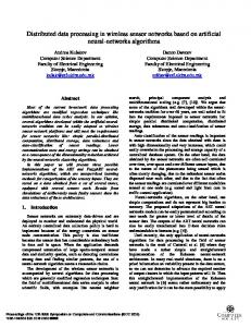
{Xd, Ymax} A’
PSEUDOCODE DUMMYREG (p, ns) begin 1. for each of the leaf nodes i of the tree a. File node”i”.dat is read b. Multivariate polynomial regression is performed on each data file
PB
PD
and the coefficients are stored in the each of the arrays
{Xmax, Yc} D
B
{Xmin, Ya}
Sensing node
Fig. 1. Illustration of how a node calculates the boundary of the region for data regeneration compression process by including readings from regions devoid of actual sensor nodes. Without any dummying i.e. without the inclusion of attribute values from non-existent nodes in the overall approximation process, error incurred is the highest. This is evident from the fact that readings that would have otherwise come from the region spanned by the non-existent nodes are not considered in the compression process. With partial dummying, a parent node follows case IV of DUMMYREG to regenerate attribute values of both of its non-existent children. But, regeneration is not done for the case when one child is present. For the full dummying case, the error incurred is minimum as attribute values are included from the entire region irrespective of whether a node is actually present or not. The lower limit of the xcoordinate (xlow) of the left child of a parent node k and the upper limit of x-coordinate (xhigh) of its right child is assumed to be u (a pre specified system parameter which depends on the size of the network) units each. When node k does not have any children, the x-coordinates of its children are approximated to lie within u units of the midpoint of the area spanned by its sensing region. Their y coordinates are assumed to be u units below that of the parent. Assuming node k to be the parent of nodes i and j, each of nodes i and j uses relation 6 to generate the coefficient tuple (β i 0 ,........, β i 8 ) and β j 0 ,........., β j 8
(
)
respectively and sends this set to node k. Node k now generates two sets of random (x, y) locations and calculates the corresponding values of the sensed attribute at each such location by using the coefficients sent by their children. These two data sets are then appended with k’s own reported readings to calculate the new set of coefficients that will be passed to k’s parent at the next higher level. This process is continued until the root node is reached which will have the final set of coefficients to be used by the sink. In this process, it is important to identify the region over which the data values are generated as they directly affect the accuracy of the approximation. We identify this region as the area bounded by the coordinates x min, y min , x max , y max , where the minimum and
{
p 2. Initialize level to while p is greater than 0 a. sum= level + 2 p − 1 b. fk=level c. while k