Mar 29, 2011 - dividual sub-matrix inverse has been computed they can be ... the individual sub-matrix inversions, where Ïâ1 ...... Colloquia Mathematica.
arXiv:1103.5782v1 [cond-mat.mes-hall] 29 Mar 2011
Distributed NEGF Algorithms for the Simulation of Nanoelectronic Devices with Scattering Stephen Cauley, Mathieu Luisier, Venkataramanan Balakrishnan, Gerhard Klimeck, and Cheng-Kok Koh School of Electrical and Computer Engineering Purdue University, West Lafayette, IN 47907-2035 Abstract Through the Non-Equilibrium Green’s Function (NEGF) formalism, quantumscale device simulation can be performed with the inclusion of electron-phonon scattering. However, the simulation of realistically sized devices under the NEGF formalism typically requires prohibitive amounts of memory and computation time. Two of the most demanding computational problems for NEGF simulation involve mathematical operations with structured matrices called semiseparable matrices. In this work, we present parallel approaches for these computational problems which allow for efficient distribution of both memory and computation based upon the underlying device structure. This is critical when simulating realistically sized devices due to the aforementioned computational burdens. First, we consider determining a distributed compact representation for the retarded Green’s function matrix GR . This compact representation is exact and allows for any entry in the matrix to be generated through the inherent semiseparable structure. The second parallel operation allows for the computation of electron density and current characteristics for the device. Specifically, matrix products between the distributed representation for the semiseparable matrix GR and the self-energy scattering terms in Σ< produce the less-than Green’s function G< . As an illustration of the computational efficiency of our approach, we stably generate the mobility for nanowires with cross-sectional sizes of up to 4.5nm, assuming an atomistic model with scattering.
1 Introduction In the absence of electron-phonon scattering, the problem of computing density of states and transmission through the NEGF formalism reduces to a mathematical problem of finding select entries from the inverse of a typically large and sparse block tridiagonal matrix. Although there has been research into numerically stable and computationally efficient serial computing algorithms [1], when analyzing certain device geometries this type of method will result in prohibitive amounts of computation and memory consumption. In [2] a parallel divide-and-conquer algorithm (PDIV) was shown to be effective for NEGF based simulations. Two applications were presented, 1
the atomistic level simulation of silicon nanowires and the two-dimensional simulation of nanotransistors. Alternative, serial computing, NEGF based approaches such as [3] rely on specific problem structure (currently not capable of addressing atomistic models), with computation limitations that again restrict the size of simulation. In addition, the ability to compute information needed to determine current characteristics for devices has not been demonstrated with methods such as [3]. The prohibitive computational properties associated with NEGF based simulation has prompted a transition to wave function based methods, such as those presented in [4]. Given an assumed basis structure the problem translates from calculating select entries from the inverse of a matrix to solving large sparse systems of linear equations. This is an attractive alternative because solving large sparse systems of equations is one of the most well studied problems in applied mathematics and physics. In addition, popular algorithms such as UMFPACK [5] and SuperLU [6] have been constructed to algebraically (based solely on the matrix) exploit problem specific structure in an attempt to minimize the amount of computation. The performance of these algorithms for the wave function based analysis of several silicon nanowires has been examined in [7]. However, for many devices of interest wave function methods are currently unable to address more sophisticated analyses that involve electron-phonon scattering. Thus, there remains a strong need to further develop NEGF based algorithms for the simulation of realistically sized devices considering these general modeling techniques. When incorporating the effects of scattering into NEGF based simulation, it becomes necessary to determine the entire inverse of the coefficient matrix associated with the device. This substantially increases both the computational and memory requirements. There are a number of theoretical results describing the structure of the inverses of block tridiagonal and block-banded matrices. Representations for the inverses of tridiagonal, banded, and block tridiagonal matrices can be found in [8–13]. It has been shown that the inverse of a tridiagonal matrix can be compactly represented by two sequences {ui } and {vi } [14–17]. This result was extended to the cases of block tridiagonal and banded matrices in [18–20], where the {ui } and {vi } sequences generalized to matrices {Ui } and {Vi }. Matrices that can be represented in this fashion are more generally known as semiseparable matrices [20, 21]. Typically, the computation of parameters {ui } and {vi } suffers from numerical instability even for modest-sized problems [22]. It is well understood that for matrices arising in many physical applications the {ui } and {vi } sequences grow exponentially [17, 23] with the index i. One approach that has been successful in ameliorating these problems, for the tridiagonal case, is the generator approach shown in [24]. Here, ratios for sequential elements of the {ui } and {vi } sequences are used as the generators for the inverse of a tridiagonal matrix. Such an approach is numerically stable for matrices of very large sizes. The extension of this generator approach to the general block-tridiagonal matrices was discussed by the same authors in [13]. The authors used the block factorization of the original block-tridiagonal matrix to construct a block Cholesky decomposition of its inverse. A generator based approach for inversion, typically referred to as the Recursive Green’s Function (RGF) algorithm, was introduced in [1] for NEGF based simulation. It is important to note that the method of [1] requires 3× less memory to compute only the density of states and transmission (in the absence of scattering), when compared 2
to the complete generator representation. In this work, we extend the approach of [2] to consider the computation of a distributed generator representation for the inverse of the block tridiagonal coefficient matrix. We then demonstrate how the distributed generator representation allows for the efficient computation of the electron density and current characteristics of the device. Our parallel algorithms facilitate the simulation of realistically sized devices by utilizing additional computing resources to efficiently divide both the computation time and memory requirements. As an illustration, we stably generate the mobility for 4.5nm cross-section nanowires assuming an atomistic model with scattering.
2 Inverses of Block Tridiagonal Matrices A block-symmetric matrix K is block tridiagonal if it has the form
A1 −BT1 K=
−B1 A2 .. .
−B2 .. . −BTNy −2
..
. ANy −1 −BTNy −1
, −BNy −1 ANy
(1)
where each Ai , Bi ∈ RNx ×Nx . Thus K ∈ RNy Nx ×Ny Nx , with Ny diagonal blocks of size Nx each. We will use the notation K = tri(A1:Ny , B1:Ny −1 ) to represent such a block tridiagonal matrix. The NEGF based simulation of nanowires using the sp3d5s∗ atomistic tight-binding model with electron-phonon scattering has been demonstrated in [25]. The block tridiagonal coefficient matrix for simulation is constructed in the following way: � K = EI − H − ΣRR − ΣRL − ΣRS .
Here, E is the energy of interest, H is the Hamiltonian containing atomistic interactions, and ΣRL , ΣRR , and ΣRS are the left and right boundary conditions and self energy scattering terms respectively. In order to calculate the current characteristics for the device we must first form the retarded Greens Function using the fact that KGR = I. A standard numerically stable mathematical representation for the inverse of this block tridiagoR
→ −
R − nal matrix is dependent on two sequences of generator matrices {g← i },{gi }. Here, → − the terms ← R − and R correspond to the forward and backward propagation through the device. Specifically, we can use the diagonal blocks of the inverse {Di } and the generators to describe the inverse a block tridiagonal matrix K in the following manner:
3
D1 R − g← 1 D1 R G = .. . 1 R − ( ∏ g← k )D1 k=Ny −1
→ − D1 g1R
···
D2
···
.. .
..
2
( ∏
R
k=Ny −1
− g← k )D2
.
···
Ny −1 → − D1 ∏ gkR k=1 Ny −1 → − R D2 ∏ g k . k=2
.. .
DNy
(2)
Where the diagonal blocks of the inverse, Di , and the generator sequences satisfy the following relationships: R
−1 − g← 1 = A1 B1 , � R R �−1 T − ← − Bi , g← i = Ai − Bi−1 gi−1
i = 2, . . . , Ny − 1,
→ −
gNRy −1 = BNy −1 A−1 Ny , � �−1 → − → − R BT R gi = Bi Ai+1 − gi+1 , i+1
i = Ny − 2, . . . , 1,
� �−1 → − D1 = A1 − g1R BT1 , � �−1 � → − → −� R BT Di+1 = Ai+1 − gi+1 I + BTi Di giR , i+1 � � → − T R DNy = A−1 I + B D g N −1 y Ny Ny −1 Ny −1 .
(3)
i = 1, ..., Ny − 2,
The time complexity associated with determining the parametrization of GR by the above approach is O(Nx3 Ny ), with a memory requirement of O(Nx2 Ny ).
2.1 Alternative Approach for Determining the Compact Representation It is important to note that if the block tridiagonal portion of GR is known, the generator → − R − can be extracted directly, i.e. without the use of entries from K sequences g R and g← through the generator expressions (3). Examining closely the block tridiagonal portion of GR we find the following relations: → −
→ −
R − g← i Di
R − g← i
Di giR = Pi =⇒ giR = D−1 i Pi ,
i = 1, . . . , Ny − 1, (4)
= Qi =⇒
=
Qi D−1 i ,
i = 1, . . . , Ny − 1,
where Pi denotes the (i, i + 1) block entry of GR and Qi denotes the (i + 1, i) block entry of GR . Therefore, by being able to produce the block tridiagonal portion of GR we have all the information that is necessary to compute the compact representation. 4
As was alluded to in Section 1, direct techniques for simulation of realistic devices often require prohibitive memory and computational requirements. To address these issues we offer a parallel divide-and-conquer approach in order to construct the compact representation for GR , i.e. the framework allows for the parallel inversion of the coefficient matrix. Specifically, we introduce an efficient method for computing the block tridiagonal portion of GR in order to exploit the process demonstrated in (4).
3 Parallel Inversion of Block Tridiagonal Matrices The compact representation of GR can be computed in a distributed fashion by first creating several smaller sub-matrices φi . That is, the total number of blocks for the matrix K are divided as evenly as possible amongst the sub-matrices. After each individual sub-matrix inverse has been computed they can be combined in a Radix-2 fashion using the matrix inversion lemma from linear algebra. Figure 1 shows both the decomposition and the two combining levels needed to form the block tridiagonal portion of GR , assuming K has been divided into four sub-matrices. In general, if K is separated into p sub-matrices there will be log p combining levels with a total of p − 1 combining operations or “steps”. The notation φ−1 i∼ j is introduced to represent the result of any combining step, through the use of the matrix inversion lemma. For example, φ−1 1∼2 is the inverse of a matrix comprised of the blocks assigned to both φ1 and φ2 . It is important to note that using the matrix inversion lemma repeatedly to join sub-matrix inverses will result in a prohibitive amount of memory and computation for large simulation problems. This is due to the fact that at each combining step all entries would be computed and stored. Thus, the question remains on the most efficient way to produce the block tridiagonal portion of GR , given this general decomposition scheme for the matrix K. In this work, we introduce a mapping scheme to transform compact representations of smaller matrix inverses into the compact representation of GR . The algorithm is organized as follows: • Decompose the block tridiagonal matrix K into p smaller block tridiagonal matrices. • Assign each sub-matrix to an individual CPU. • Independently determine the compact representations associated with each submatrix. • Gather all information that is needed to map the sub-matrix compact representations into the compact representation for GR . • Independently apply the mappings to produce a portion of the compact representation for GR on each CPU. The procedure described above results in a “distributed compact representation” allowing for reduced memory and computational requirements. Specifically, each CPU will
5
Decomposition
Sub−matrix Inversion
Combining Level: 1
Combining Level: 2
Compact Representation
−1
φ1
K
φ1
−1
K
−1
φ1
−1
φ 1~2
−1
φ2
−1
φ2
φ2 −1
φ3
−1
φ3
φ3
−1
φ 3~4
−1
φ4
−1
φ4
φ4
Matrix Maps
Figure 1: Decomposition of block tridiagonal matrix K into four sub-matrices, where the shaded blocks correspond to the bridge matrices. The two combining levels follow the individual sub-matrix inversions, where φ−1 i∼ j represents the inverse of divisions φi through φ j from the matrix K. Matrix mappings will be used to capture the combining effects and allow for the direct computation of the block tridiagonal portion of GR .
eventually be responsible for the elements from both the generator sequences and diagonal blocks that correspond to the initial decomposition (e.g. if φ1 is responsible for blocks 1, 2, and 3 from the matrix K, the mappings will allow for the computation of → −
R
R , g← − g1...3 1...3 , and D1...3 ). In order to derive the mapping relationships needed to produce a distributed compact representation, it is first necessary to analyze how sub-matrix inverses can be combined to form the complete inverse. Consider the decomposition of the block tridiagonal matrix K into two block tridiagonal sub-matrices and a correction term, demonstrated below:
K=
� φ1 |
φ2 {z K˜
�
+ XY,
}
φ1 = tri(A1:k , B1:k−1 ),
X=
� 0 ··· 0 ···
−BTk 0
φ2 = tri(Ak+1:Ny , Bk+1:Ny −1 ), 0 −Bk
··· ···
and
�T � 0 0 ··· ,Y= 0 0 ···
0 I
I ··· 0 ···
� 0 . 0
Thus, the original block tridiagonal matrix can be decomposed into the sum of a block diagonal matrix (with its two diagonal blocks themselves being block tridiagonal) and a correction term parametrized by the Nx × Nx matrix Bk , which we will refer to as the “bridge matrix”. Using the matrix inversion lemma, we have GR = (K˜ + XY )−1 = K˜ −1 − (K˜ −1 X) I + Y K˜ −1 X
6
�−1
(Y K˜ −1 ),
where K˜ −1 X I + Y K˜ −1 X
�−1
Y K˜ −1
� −1 � −φ1 (:, k) Bk 0 T , 0 −φ−1 2 (:, 1) Bk � � T −1 I −φ−1 2 (1, 1) Bk = , −φ−1 I 1 (k, k) Bk � T� 0 φ−1 2 (:, 1) , = T φ−1 0 1 (:, k) =
(5)
−1 −1 and φ−1 1 (:, k) and φ2 (:, 1) denote respectively the last and first block columns of φ1 and φ−1 2 . This shows that the entries of K˜ −1 are modified through the entries from the first −1 rows and last columns of φ−1 1 and φ2 , as well as the bridge matrix Bk . Specifically, since φ1 is before or “above” the bridge point we only need the last column of its inverse to reconstruct GR . Similarly, since φ2 is after or “below” the bridge point we only need the first column of its inverse. These observations were noted in [2], where the authors demonstrated a parallel divide-and-conquer approach to determine the diagonal entries for the inverse of block tridiagonal matrices. We begin by generalizing the method from [2] in order to compute all information necessary to determine the distributed compact representation of GR (3). That is, we would like to create a combining methodology for sub-matrix inverses with two major goals in mind. First, it must allow for the calculation of all information that would be required to repeatedly join sub-matrix inverses, in order to mimic the combining process shown in Figure 1. Second, at the final stage of the combining process it must facilitate the computation of the block tridiagonal portion for the combined inverses. Details pertaining to the parallel computation of GR are provided in Appendix A. The time complexity of the algorithm � presented is O(Nx3 Ny /p + Nx3 log p), with memory consumption O Nx2 Ny /p + Nx2 . The distribution of the compact representation is at the foundation of an efficient parallel method for calculating the less-than Green’s Function G< and greater-than Green’s Function G> .
4 Parallel Computation of the Less-than Green’s Function The parallel inversion algorithm described in Section 3 not only has advantages in computational and memory efficiency but also facilitates the formulation of a fast, and highly scalable, parallel matrix multiplication algorithm. This plays an important role during the simulation process due to the fact that computation of the less-than Green’s Function requires matrix products with the retarded Green’s Function matrix: ∗
G< = GR Σ< GR .
(6)
Σ< , which we will refer to as the less-than scattering matrix, is typically assumed to be a block diagonal matrix. We will demonstrate how the distributed compact representa7
tion of the semiseparable matrix GR presented in Section 3 can be used to calculate the necessary information from G< . Specifically, the electron density for the device will be calculated through the diagonal entries of G< and the current characteristics through the first off-diagonal blocks of G< .
4.1 Mathematical Description Recall that our initial state for this procedure would assume that portions of the block tridiaongal (corresponding to the size and location of the divisions) of GR have been calculated and stored. It is important to note that there are many generator representations for GR and we would like to select a representation that will facilitate efficient calculation of G< . For the mathematical operation shown in (6), our starting point will � → − �T R − be describing the kth block row of GR in terms of Di , giR , and g← i , the diagonal blocks and two generator sequences respectively. The following expressions are used to determine the generators from the block tridiagonal of the semiseparable matrix: R
R
−1 − ← − Pi = g← i Di+1 ⇒ gi = Pi (Di+1 ) ,
� → � → − �T − �T Qi = giR Di ⇒ giR = Qi (Di )−1 .
(7)
Di , Pi , and Qi , are the diagonal, upper diagonal, and lower diagonal blocks respec� → − �T R th − tively. Thus, the generators giR and g← i are used to describe the k block row of GR semiseparable matrix in the following way: GR (k, :) = � 1 � − → �T ∏ giR D1 i=k−1
···
� → − �T R Dk−1 gk−1
Dk
R − g← k Dk+1
Ny −1
··· ∏
i=k
R − g← i DNy
�
This generator representation for GR along with the block diagonal structure of Σ< allows for us to express each diagonal block of G< in terms of recursive sequences. Both → − < − the forward recursive sequence gi< and backward recursive sequence g← i are dependent on a common sequence of injections terms Ji (note: the arrow orientation for g< matches that of gR ). The relationships between the sequences and the diagonal blocks of G< are shown below:
8
∗ Ji = Di Σ< i Di ,
i = 1, 2, . . . , Ny
→ −
g1< = J1 � → − �C − �T → → − − � → R R < gi−1 gi< = Ji + gi−1 , gi−1
i = 2, . . . , Ny