Jan 27, 2008 - known benchmarks including shocks, the Weibel instability, Landau ... ven), by the European Commission through the SOLAIRE network ...
**FULL TITLE** ASP Conference Series, Vol. **VOLUME**, **YEAR OF PUBLICATION** **NAMES OF EDITORS**
arXiv:0801.4134v1 [physics.comp-ph] 27 Jan 2008
The algorithms of the implicit method Giovanni Lapenta Centrum voor Plasma-Astrofysica, Departement Wiskunde, Katholieke Universiteit Leuven, Celestijnenlaan 200B - bus 2400, B-3001 Heverlee, Belgi¨e. Abstract. We discuss the fundamentals of the implicit moment method for Particle In Cell (PIC) simulation as presently implemented in the CELESTE3D code. We present the method in its fully electromagnetic and fully kinetic version. The application of the method is to problems with multiple temporal and spatial scales, common in all space, astrophysical and laboratory plasmas.
1.
Introduction
The implicit particle in cell (PIC) method was developed as a general plasma simulation tool based on a fully kinetic approach (Mason 1981; Denavit 1981) that did not rely on any physical approximation but only on the use of advanced numerical methods to reduce the cost of large scale kinetic simulations. In its simplest form the PIC method uses explicit time discretization methods (Birdsall and Langdon 2004). The equations of motion need the fields acting on the computational particles and the field equations need the moments computed from the particles. The great majority of PIC codes in use today address this problem relying on a explicit method. In the explicit method, the field equations are discretized with one in a number of different explicit methods available (see Birdsall and Langdon (2004); Hockney and Eastwood (1988) for a review) and the equations of motion are usually discretized with the leap-frog algorithm (Birdsall and Langdon 2004; Hockney and Eastwood 1988). The key point is that in the explicit method, the field equations need only the sources from the previous time cycle and the equations of motions need only the fields from the previous time cycle. Even though the equations remain coupled, no iteration is needed and the cycle becomes a simple marching order where each block is applied after its predecessor and needs only information already available. This choice makes the explicit PIC very simple. As can be imagined this simplicity comes at a price. The explicit PIC approach is subject to three very restrictive stability constraints. First, the explicit discretization of the field equations requires that a Courant condition must be satisfied on the speed of light: c∆t < ∆x
(1)
Second, the explicit discretization of the equations of motion introduces a constraint related to the fastest electron response time, the electron plasma frequency: ωpe ∆t < ∆x (2) 1
2
Giovanni Lapenta
Note that, instead, thanks to the Boris algorithm for the motion in a magnetic field, the gyromotion introduces no stability constraints (Birdsall and Langdon 2004). Finally, the interpolation between grid and particles causes a loss of information and an aliasing instability called finite grid instability that results in an additional stability constraint: ∆x < ςλDe
(3)
that requires the grid spacing to be of the order of the Debye length or smaller, the proportionality constant ς being of order one and dependent on the details of the scheme used (Birdsall and Langdon 2004; Hockney and Eastwood 1988). Thanks to ever faster computers, the explicit PIC method has been able to achieve remarkable results. But there are problems where multiple scales still prevent its use. When the interest is on large scales and slow processes other approaches are needed. The implicit PIC approach provides a viable alternative in such cases. 2.
Implicit PIC
The implicit PIC method has been developed along two different lines of investigation: the direct implicit method (Langdon et al. 1983) and the implicit moment method (Brackbill and Forslund 1982). Here we consider the implicit moment method. In the last few years, we have published a number of papers on the application of CELESTE3D and a full description of the methods used has been provided by Lapenta et al. (2006). In the present work, we summarize the latest status of the implicit moment method as implemented in CELESTE3D. We consider first the time discretization. The solution is advanced in time with discrete steps, ∆t, from the initial time, t0 = 0 to the final time tN = T . The generic quantity Ψ at time step n (t = tn ), is denoted with Ψn . The equations of motion are discretized as (Vu and Brackbill 1992): xn+1 = xnp + vpn+1/2 ∆t p vpn+1
=
vpn
� qs ∆t � n+θ n+1/2 + Ep (xp ) + vpn+1/2 × Bnp (xpn+1/2 ) ms
(4)
where all quantities evaluated at intermediate levels are computed as: Ψn+θ = Ψn (1−θ)+Ψn+1 θ. Note that the velocity equation is more conveniently rewritten as: b n+θ (xn+1/2 ) bp + βs E vpn+1/2 = v (5) p p
where βs = qp ∆t/mp (independent of the particle weight and unique to a given species). For convenience, we have introduced hatted quantities obtained by explicit transformation of quantities known from the previous computational cycle: bp = αns · vpn v (6) b n+θ = αn · En+θ E s s s
Implicit Moment PIC
3
The transformation tensor operators αns are defined as: αns =
� 1 n 2 n n I − β I × B + β B B s s 1 + (βs B n )2
(7)
and represent a scaling and rotation of the velocity vector. The semi–discrete (continuous in space) temporal discretization to Maxwell’s equations is written as: ∇ × En+θ + ∇ × Bn+θ −
1 Bn+1 − Bn =0 c ∆t
1 En+1 − En 4π n+ 1 = J 2 c ∆t c
(8)
∇ · En+θ = 4πρn+θ ∇ · Bn = ∇ · Bn+1 = 0, The parameter θ ∈ [1/2, 1] is chosen in order to adjust the numerical dispersion relation for electromagnetic waves (for θ < 1/2, the algorithm is shown to be unstable (Brackbill and Forslund 1982)). We note that for θ = 1/2 the scheme is second-order accurate in ∆t; for 1/2 < θ ≤ 1 the scheme is first-order accurate. The sources in Maxwell’s equations necessitate information from the particles: P s ρs = N p=1 qp W (x − xp ) (9) P s q v W (x − x ) Js (r) = N p p=1 p p where the species is labelled by s and the sums are carried over all particles of a species Ns . The coupling with the particle equations of motion is evident. The fundamental problem to address in developing an implicit PIC method is the coupling between the equations of motion and the field equations for the presence of the time advanced electric field (but not magnetic field, that is used from the previous cycle, as no instability is introduced) in the equations of motion and for the appearance of the particle properties in the sources of the Maxwell equations. In both cases the coupling is implicit, so that the new particle properties need to be known before the fields can be computed and likewise the new fields need to be available before the new particle properties can be computed. 3.
Implicit Moment Method
The implicit moment method removes the need for iterative methods and provides a direct method to compute the advanced fields without first having to move the particles. The implicit moment method reduces the number of equations that must be solved self-consistently to a set of coupled fluid moment and field equations. The solution of these equations implicitly, and the subsequent
4
Giovanni Lapenta
solution of the particle equations of motion in the resulting fields, is stable and accurate. The coupling due to the implicit discretization of both field and particle equations is approximated, representing the sources of the field equations using the moment equations instead of the particle equations directly. Once the field equations are solved within this approximation, the rest of the steps can be completed directly without iterations: with the new fields, the particle equations of motion can be solved and the new current and density can be computed for the next computational cycle. The implicit moment method formulation used here is described in details by Brackbill and Forslund (1982); Lapenta et al. (2006). The key step is to derive a suitable set of moment equations that can approximate the particle motion over a computational cycle. The approach followed in the present implementation is based on a series expansion of the interpolation functions used to transfer information between grid and particles. The details of the simple but demanding algebraic manipulations are provided by Vu and Brackbill (1992), the final answer being: n+1/2 = ρns − ∆t∇ · Js ρn+1 s (10) n+1/2 ∆t ∆t b b Js = Js − 2 µs · Eθ − 2 ∇ · Πs
where the following expressions were defined:
b s = P qp v bp W (x − xnp ) J p
b s = P qp v bp v bp W (x − xnp ) Π p
(11)
with the obvious meaning, respectively, of current and pressure tensor based on the transformed hatted velocities. An effective dielectric tensor is defined to express the feedback of the electric field on the plasma current and density: µns = −
qs ρns n α ms s
(12)
The expression (10) for the sources of the Maxwell’s equations provide a direct and explicit closure of Maxwell’s equations. When eq. (10) is inserted in eq. (8), the Maxwell’s equations can be solved without further coupling with the particle equations. This is the key property of the moment implicit method and allows the implicit moment PIC method to retain the once-through approach typical of explicit methods and eliminates the need for expensive iteration procedures that would require to move the particles multiple times per each computational cycle. 4.
Stability
The stability properties of the method described above have been studied extensively in the past (Brackbill and Forslund 1982). All the stability constraints
Implicit Moment PIC
5
discussed above for the explicit method are removed. The implicit particle mover removes the need to resolve the electron plasma frequency, and the implicit formulation of the field equations removes the need to resolve the speed of light. The time step constraints are replaced by an accuracy limit arising from the derivation of the fluid moment equations using the series expansion. This limit restricts the mean particle motion to one grid cell per time step (Brackbill and Forslund 1982), i.e. vth,e ∆t/∆x < 1, (13) The finite grid instability limit for the explicit method, ∆x < ςλDe is replaced by (Brackbill and Forslund 1982) ∆x/∆t < ςvth,e ,
(14)
that allows large grid spacings to be used when large time steps are taken. The gain afforded by the relaxation of the stability limits is two-fold. First, the time step can far exceed the explicit limit. In a typical plasma the electron plasma frequency is far smaller than the time scales of interest and its accurate resolution is not needed. Within the current approach, the processes developing at the sub-∆t scale are averaged and their energy is damped by a numerically-enhanced Landau damping. In other approaches, such as the gyrokinetic or hybrid approach (Lipatov 2002), such processes are completely removed and the energy channel towards them is interrupted, removing for example the possibility to exchange energy between sub-∆t fluctuations and particles. In the implicit approach, instead, the sub-∆t scales remain active and the energy channel remains open. This is a crucial feature to retain a full kinetic approach. Furthermore, when additional resolution of the smallest scales is needed, the implicit method can access the same accuracy of the explicit method simply using a smaller time step and grid spacing. This feature is not accessible to reduced models, e.g. gyroaveraged methods, that remove the small scales entirely. Second, the grid spacing can far exceed the Debye length. Often the scales of interest are much larger than the Debye length. The ability to retain a full kinetic treatment without the need to resolve the Debye length results in a much reduced cost for the implicit PIC method. 5.
Conclusions
The implicit moment PIC method described above is implemented in the CELESTE3D code. The CELESTE3D code was originally conceived for the numerical tokamak project (Brackbill and Lapenta 1994) but has found its main application in space physics. Four types of tests have been conducted to verify and validate CELESTE in full 3D cartesian geometry and in reduced geometries in 2D and 1D: 1) well known benchmarks including shocks, the Weibel instability, Landau damping and ion acoustic waves (Vu and Brackbill 1992); 2) the GEM challenge (Ricci et al. 2002b,a) and the Newton challenge (Birn et al. 2005); 3) study of reconnection in systems with low betas, investigating the reconnection process both at the macroscopic and microscopic level obtaining agreement with the explicit PIC code NPIC (Ricci et al. 2004a); 4) 3D stability study of a current sheet
6
Giovanni Lapenta
Figure 1. 3D Simulation of the magnetotail requiring 1 day of CPU time on CELESTE3D or 800,000 years on a explicit code
equilibrium, compared with satellite observations obtained from the CLUSTER and GEOTAIL mission (Lapenta and Brackbill 2002; Lapenta et al. 2003; Ricci et al. 2004b). As an example of this last case, we show here the results of an actual simulation conducted in 3D of a system initially in the magnetotail equilibrium described by Birn (1987). The physics developing in the simulation includes first the growth and saturation of the lower hybrid drift instability, followed by the onset of reconnection and current flapping leading to the macroscopic restructuring of the topological configuration of the magnetotail. The physics steps of the process are described in deatils by Lapenta and Brackbill (2002, 2000); Lapenta et al. (2003); Ricci et al. (2004b). The fundamental consideration of interest here is the efficacy of the simulation approach. In a typical explicit run, the time step would have to be selected according to the stability constraint of ωpe ∆t < 2. In a typical magnetotail case, the electron plasma frequency is of the order of ωpe ≈ 5 · 104 s−1 , and the ion plasma frequency is of the order of ωpi ≈ 103 s−1 , both smaller than the smallest scale of interest for this problem which is the lower hybrid frequency range of ωLH ≈ 102 s−1 . In a implicit simulation, we can select the time step to the ion plasma frequency, still resolving accurately the lower hybrid range, but saving two orders of magnitude compared with the explicit case that instead is needlessly resolving the electron plasma scale. A similar gain occurs in each spatial direction. In a explicit simulation, for stability the grid spacing needs to satisfy ∆x/λDe < ς. The Debye length in the magnetotail is of the order of 100m. But the smallest scales of interest in the present case are in the range between the electron (10km) and the ion (100km) inertial scales or gyroscales. In our simulation we set the resolution at 10km, saving two orders of magnitude in each spatial direction but still resolving the important scales. Counting all savings, we have saved 2 orders of magnitude in each spatial direction and in time (in total 8 orders of magnitude), without loosing the deatils
Implicit Moment PIC
7
of the scales of interest. The savings means that on the same computer, an implciti simulation can compute in one day what an explicit simulation would require nearly 800,000 years. Acknowledgments. The author is very grateful to Jerry Brackbill and Paolo Ricci for the collaboration in all the work summarized here. The present work is supported by the Onderzoekfonds K.U. Leuven (Research Fund KU Leuven), by the European Commission through the SOLAIRE network (MRTN-CT2006-035484), by the NASA Sun Earth Connection Theory Program and by the LDRD program at the Los Alamos National Laboratory. Work performed in part under the auspices of the National Nuclear Security Administration of the U.S. Department of Energy by the Los Alamos National Laboratory, operated by Los Alamos National Security LLC under contract DE-AC52-06NA25396. Simulations conducted in part on the HPC cluster VIC of the Katholieke Universiteit Leuven. References Birdsall, C. and Langdon, A.: Plasma Physics Via Computer Simulation, Taylor & Francis, London, 2004. Birn, J.: J. Geophys. Res., 92, 11 101–11 108, 1987. Birn, J., Galsgaard, K., Hesse, M., Hoshino, M., Huba, J., Lapenta, G., Pritchett, P. L., Schindler, K., Yin, L., Buchner, J., Neukirch, T., and Priest, E. R.: Geophys. Res. Lett., 32, L06 105, 2005. Brackbill, J. and Forslund, D.: J. Comp. Phys., 46, 271, 1982. Brackbill, J. and Lapenta, G.: The Effect of Shape on the Ion Temperature Gradient Instability, Bull. Am. Phys. Soc., 39, 1665–1666, 1994. Denavit, J.: J. Comp. Phys., 42, 337, 1981. Hockney, R. and Eastwood, J.: Computer simulation using particles, Taylor & Francis, London, 1988. Langdon, A., Cohen, B., and Friedman, A.: J. Comp. Phys., 51, 107–138, 1983. Lapenta, G. and Brackbill, J.: Nonlinear Processes Geophys., 7, 151, 2000. Lapenta, G. and Brackbill, J.: Phys. Plasmas, 9, 1544–1554, 2002. Lapenta, G., Brackbill, J. U., and Daughton, W. S.: Phys. Plasmas, 10, 1577–1587, 2003. Lapenta, G., Brackbill, J. U., and Ricci, P.: Phys. Plasmas, 13, 5904, 2006. Lipatov, A. S. S.: The Hybrid Multiscale Simulation Technology, Springer, Berlin, 2002. Mason, R.: J. Comp. Phys., 41, 233, 1981. Ricci, P., Lapenta, G., and Brackbill, J.: Geophys. Res. Lett., 29, 10.1029/2002GL015314, 2002a. Ricci, P., Lapenta, G., and Brackbill, J.:J. Computat. Phys., 183, 117–141, 2002b. Ricci, P., Brackbill, J., Daughton, W., and Lapenta, G.: Phys. Plasmas, 11, 4102–4114, 2004a. Ricci, P., Lapenta, G., and Brackbill, J.: Geophys. Res. Lett., 31, L06801, 2004b. Vu, H. X. and Brackbill, J. U.: Comp. Phys. Comm., 69, 253, 1992.