Sep 20, 1993 - p2 pn t1' (alfa1', beta1') pn+1 pn+2 pn+m p1 p2 pn t (alfa,beta) pn+1 pn+2 pn+m t2' (alfa2', beta2') p. Timing Contraints Event Transformation.
IPTES Project EP5570
Hierarchical Decomposition of High Level Timed Petri Nets
Author: Miguel Felder, Carlo Ghezzi, Mauro Pezz�e Date: September 20th, 1993 Doc. Id.: IPTES-PDM-54-V2.0 Work Package/Task No.: NWP1/T4.1-T4.2
IPTES Project
The objective of the IPTES (Incremental Prototyping Technology for Embedded Real-Time Systems) project is to develop methodologies, tools and theoretical results on distributed prototyping for realtime systems. IPTES is partially funded by the European Communities under the ESPRIT programme, project nos. EP5570 and EP7811.
IPTES Consortium
IFAD - The Institute of Applied Computer Science VTT - Technical Research Centre of Finland PDM - Politecnico di Milano MARI Computer Systems Limited DIT/UPM - Universidad Polit�ecnica de Madrid TS - T�el�esystemes TID - Telef�onica Investigaci�on y Desarrollo CEA/LETI - Commissariat a� l'Energie Atomique ENEA - Ente per Energia & Ambiente RNT - Rautaruukki New Technology
Denmark Finland Italy UK Spain France Spain France Italy Finland
Type: Status: Availability: Copyright:
IPTES.Report Final Public
c 1993 PDM
Document History V1.0 V2.0
Original Version Final version. Corrected according to the suggestions of the internal reviewers, discussed at TCC19 (Milan, September 15-16th, 1993).
Abstract In IPTES, real-time system speci cations expressed in SA/SD-RT are internally represented by means of High Level Timed Petri Nets (HLTPNs). Petri nets present several widely recognized advantages, however their usefulness is limited by the absence of hierarchical decomposition mechanisms. The absence of hierarchical decomposition mechanisms has at least three main consequences on the usability of Petri nets for the speci cations of real size systems: fast growth of the speci cations that become quickly unreadable: impossibility of mapping the hierarchical aspects of speci cations expressed in a hierarchical language (e.g. SA/SD-RT) directly onto Petri nets; no support for reducing the analysis e�ort by means of divide and conquer strategies based on a suitable hierarchy. This report presents a formal hierarchical decomposition mechanism for HLTPNs, that it can enhance existing analysis techniques, support mapping from hierarchical speci cation languages, and improve the readability of large speci cations. This report de nes the conditions under which the properties that are proven to hold at a given abstraction level are preserved at the next re ned level. To do so, we de ne the concept of correct re nement, and we show that interesting temporal properties are preserved by correct re nements. We also provide a set of constructive rules that may be applied to re ne a net in such a way that the resulting net is a correct re nement. Finally the report sketches the main features of a rst prototype built as part of the IPTES project.
Contents
1 2 3 4 5 6 7 8
Introduction Notation and Properties Observable Time Behavior Implementation Relation Re nement Rules The Prototype Conclusions References
IPTES-PDM-54-V2.0
2 4 6 8 10 15 21 21
1
1 Introduction The IPTES end-user speci es real-time system by means of speci cation techniques suggested by the SA/SD-RT methodology ([Ward&85]). Such speci cations are mapped onto a formal kernel model (High Level Timed Petri Nets - HLTPNs), so that ambiguities that may raise by the use of semiformal speci cation languages (such as the one proposed by the SA/SD-RT methodology) are solved. The IPTES platform provides several analysis techniques based on the formal kernel model. The analysis results are always presented to the end-users in terms of their speci cation language, so that the end users can even ignore the existence of the formal kernel and still take advantage for it. Petri nets present several widely recognized advantages, however their usefulness is limited by the absence of hierarchical decomposition mechanisms. The absence of hierarchical decomposition mechanisms has at least three main consequences on the usability of Petri nets for the speci cations of real size systems:
� fast growth of the speci cations: the Petri net speci cations of even small systems
�
�
1
quickly become too large to be kept on the screen and to be understand by the enduser. This makes Petri nets di�cult to be directly used for the speci cation of real size system, whenever speci cations are used as a means of communication among people involved in the analysis and development. This is not a big disadvantage for the IPTES end-users that can even ignore the underlying Petri nets. impossibility of mapping speci cations expressed in any hierarchical language directly onto Petri nets. Only non-hierarchical aspects can be directly mapped onto Petri nets, while all hierarchy related aspects are lost in the mapping. This is potentially a serious limitation in the IPTES framework, which is based on hierarchical end-user speci cation languages automatically mapped onto nets. Presently, such inconvenience is solved by mapping only the " atten" speci cation (i.e. the speci cation without hierarchy) onto HLTPNs. However, we believe that the needs of mapping the hierarchy as well can become crucial for further development of the IPTES methodology and toolset. no support for reducing the analysis e�ort by means of divide and conquer strategies based on a suitable hierarchy. A suitable hierarchy could largely reduce the e�ort needed for analysing real size speci cations by requiring the analysis technique to be applied only to the top of the hierarchy, i.e. on a reasonably small speci cation. The lack of support for analysis is not a crucial point as far as the end-user only refers to testing and simulation, and uses some high level hierarchical interface (e.g., SA/SD-RT). However in some cases, part of the system may be so critical to require more reliable analysis techniques. In such cases, the possibility of applying techniques for formally proving the validity of the required properties may become a key feature for the success of the methodology and the toolset. Moreover, we believe that a skilled user will highly appreciate the simulation and testing facilities o�ered by IPTES at the rst impact, but he/she will appreciate even more formal proof techniques as far as he/she proceeds in the speci cation and analysis of large critical systems, thus becoming a next generation user of IPTES 1.
We would like to stress here that this last statement re ects the opinion of PDM and some other
IPTES-PDM-54-V2.0
2
Recently, some attempts to de ne hierarchical extensions of Petri net have been made. Unfortunately, none of them is fully satisfactory in the IPTES framework. Some of them are only syntactical (e.g. [Huber&89]). Hierarchies de ned only syntactically help in keeping the growth of the speci cation at a reasonable level, but do not provide an acceptable support for mapping hierarchical speci cation languages onto Petri nets nor for supporting formal proof of properties. The few attempts to provide a formal basis to the hierarchy do not deal with time and are usually too strict to provide a reasonable platform to base the representation of hierarchies as needed when modeling real size systems ([Vogler90, Glabbeek&90, Damm&90, Aizikowitz90]). This report presents a hierarchy for HLTPNs. The hierarchy de ned in this report di�ers from previous proposals in many aspects:
� the reference model: we deal with HLTPNs and not only with traditional Petri
� �
�
nets as most of the previous attempts (an exception being represented by [Huber&89], that deals with Colored Petri nets. However, [Huber&89] proposes only a syntactically de ned hierarchy). Actually we deal with a subset of HLTPNs; basically the semantics of correct re nement is de ned with respect to temporal properties and thus it takes into account only temporal information and ignores data, consistently with the work done on analysis within the IPTES project ([Bellettini&93]). All the concepts de ned in this report can be applied to HLTPNs that includes data and functionalities, but the consistency of the re nement is de ned only with respect to the temporal information, that is a re nement proven to be correct with respect to the de nitions presented in this report may be wrong with respect to data and functional information. This limits the bene ts of using the rules de ned in this report to the IPTES methodology. it relies on a formally de ned basis, i.e. if a net N 0 is shown to be a correct re nement of a net N according to the de nition presented in this report, the temporal properties proven for net N are guaranteed to be valid for net N 0 as well. it allows a net initially fairly small to become larger and larger. This overcomes one of the major disadvantages of many de nitions of equivalence that lead to hierarchies. Such de nitions often preserve far more properties, but greatly limit the changes in the initial net so that they are of little interest for practical applications where the speci cation starts with a small de nition that grows by adding a great amount of details ignored in the rst speci cation. it has been used for building an early prototype that we plan to use for investigating real size examples. Unfortunately, due to higher priorities within the project a lot of e�ort initially planned for to this task has been moved to more critical tasks with the result of greatly restricting the production of a prototype and its validation within this project.
partners, but not all the partners hold with this way of thinking. We like to consider this as the di�erence between a long term goal, maybe not satis able at the industrial level now, versus a more concrete view that gives high priority to tools and techniques that are current status of the art. We maybe wrong. Anyway, we believe that the work documented in this report adds value to the IPTES project despite the dispute on this last topic, considering potential advantages in mapping hierarchical speci cation languages on HLTPNs.
IPTES-PDM-54-V2.0
3
This report is organized as follows. Section 2 shows the basic restrictions on HLTPNs that we consider in this report. It also presents the temporal properties we referred to while de ning property preserving transformations. The main restrictions to HLTPNs and the properties are fully consistent with the one used in the analysis toolset de nition and implementation. The reader familiar with [Bellettini&93] can skip this section. Some restrictions may appear too strong. In particular, excluding functions data and predicates may a�ect the applicability of the rules de ned in this report to interesting cases that the IPTES methodology addresses. The restrictions are due to the cuts on the overall e�ort spent in tasks T4.1 and T4.2 2 , resulting in not enough e�ort for coping with the more general problem. The reminder of the report is organized in two major parts: the rst part, including Sections 3 and 4, presents general de nitions; the second part, including Section 5, presents a set of re nement rules that can be immediately applicated to concrete examples. The general de nitions introduced in the rst part refer to a general model (HLTPNs with the restrictions described in Section 2) and are essential for proving the correct semantics of the rules de ned in the second part. The rules de ned in the second part have been proven correct only in speci c situations. Such situations are partially given rule by rule as hypothesis for the applicability of the speci c rule, and partially given for the whole set of rules. In particular, the restrictions for the whole set of rules are given by referring to a subset of HLTPNs, called MF nets. However, despite the re nement rules practically applicable given in Section 5 are de ned for the special case of MF nets, the general de nitions given in Section 3 and 4 can be used for de ning additional rules for HLTPNs not restricted to MF nets only. Sections 6 and 7 conclude brie y by describing an early prototype, and presenting possible extensions of the work described in this report.
2 Notation and Properties The hierarchical decomposition techniques presented in this report has been de ned and implemented using a notation that slightly di�ers from the notation used in [Felder&92]. The new notation is consistent with the notation used in [Ghezzi&91] and [Bellettini&93] that describe the analysis algorithm and toolset. In particular, the notation used in this report di�ers from HLTPNs for what concern the basic model which is a subset of HLTPNs. HLTPNs have been slightly restricted in order to cope with the complexity of the problem. The main restrictions concern data, that are simply ignored. The hierarchy de ned in this report only preserves temporal properties, and thus it deals only with timing information. All the supporting functionalities has been provided by an existing tool: Cabernet3 . The use of Cabernet made possible the implementation of the initial prototype with the available resources. Here we brie y describe the notation used in this document referring to the simple example of Figure 1, that will be used through the whole report. The net of Figure 1 represents a simple producer/consumer system. The producer gets data (e.g., temperature, pressure) from an external device and then it communicates the acquired The e�ort taken away from tasks T4.1 and T4.2 has been used for de ning the mapping of SA/SDRT to HLTPNs, a task more critical for the completion of the IPTES platform. 3 Cabernet is part of the IPTES background. 2
IPTES-PDM-54-V2.0
4
p2 (ready for elaboration) p1 (ready for acquisition)
t1 (acquisition)
t2 (communication)
p3 (ready for communication)
t3 (elaboration)
p4 (ready for communication)
t1 hp1 + 5; p1 + 10i Time-Functions: t2 henab + 2; enab + 5i t3 hp2 + 6; p2 + 8i
Figure 1: A simple HLTPN: a producer/consumer system, a high-level speci cation. data to the consumer, which is responsible for the elaboration. Time functions are expressed as pair of functions representing the minimum and maximum ring time of the transition, respectively. Time functions refer to the time stamps of the tokens in the preset of the transition by means of the name of the place. For instance, the time function associated with transition t1 (hp1 + 5; p1 + 10i) indicates that transition t1 , that represents the producer acquiring a datum, res not before 5 and not later than 10 time units after place p1 has been marked. The special identi er enab is used to indicate the maximum among the timestamps associated with the tokens concurring in enabling the transitions. For instance, the time function associated with transition t2 (henab + 2; enab + 5i) indicates that transition t2, representing the communication between consumer and producer, res between 2 and 5 time units after both places p3 and p4 have been marked. The elaboration of the consumer takes 6 to 8 time units (transition t3). In the initial marking (shown in Figure 1), the producer is ready for acquiring a new datum and the consumer is ready for elaborating the last received datum. From now on, for simplicity, we will implicitly assume that all marked places in the initial marking contain tokens whose timestamp are zero. In this report we consider two di�erent time semantics: Monotonic Weak Time Semantics (MWTS), and Strong Time Semantics (STS). Under MWTS enabled transitions are not forced to re, i.e. a transition t may never re, despite being enabled in a given interval and not being disabled by any other ring. MWTS only requires occurrence of rings in ring sequences to be ordered with respect to the occurrences of the rings on the time axis. Under STS an enabled transition is forced to re unless disabled by the ring of another transition before the latest ring time of t. Presently, IPTES refers only to STS. This report is thus more general than strictly required. The added generality does not limit the results and makes them applicable to a wider class of cases and possible extensions. Any formal de nition of hierarchical decomposition relies on a set of properties that are preserved by the re nement relation. Since IPTES supports the development of real-time systems, interesting properties to be preserved include temporal properties. The re nement relation de ned in this document preserve temporal properties that we can formally prove for HLTPN speci cations, namely bounded invariance and bounded IPTES-PDM-54-V2.0
5
response properties. A bounded invariance property asserts a property that is veri ed in all the states reached within a given time limit. For example the nuclear reactor control system always being in a safe state within a given deadline is a bounded invariance property. A bounded-response property asserts that a property eventually holds before a given time is reached. In the case of the net of Figure 1, the requirement that, once a datum is acquired, it will be elaborated within a given time (e.g. 25 time units), is a bounded-response property.
3 Observable Time Behavior The purpose of HLTPNs speci cations is to provide a formal description of temporal behaviors of a given system. Behaviors, in a given nite time interval, can be described by transition rings occurring on the temporal axis. According to this view, rings are the only externally observable elements. The structure of the net, including the causal relation among rings, are indeed hidden. In HLTPNs, there is no explicit concept of clock; time progresses only as rings occur. When we observe a ring sequence � , we can say that we are at time � , if � is the ring time of the last ring of � . In order to de ne the behavior of a system within a given time interval, let us introduce �(N; � ), the set of observable ring sequences within a given time limit. The de nition works in the context of both MWTS and STS. Informally, �(N; � ) represents the set of all possible behaviors of the net that an external user can observe within a nite time, i.e. the set of all possible ring sequences \cut" to the time limit � . The formal de nition presented below requires the net to be augmented with a simple subnet that guarantees to consider only \complete" sequences up to the time limit. In particular the added subnet ensures that all strong transitions that must re at time � (the time limit) belong to the considered sequences. �(N; � )
De nition 1 (�(N; � ): Set of ring sequences of HLTPN N observable until � ) Given
a HLTPN N and a time value � , let � (called cut value) be any value with � > � . We rst modify N by adding two new places p1 , p2 (place p1 marked with a token) and a transition t, which is an output transition for p1 and an input transition for p2 . The time-function associated with t is the constant �. Let N� be the resulting net, and let �t be the set of N� 's ring sequences whose last ring occurrence is t's ring. �(N; � ) is de ned as the smallest set that contains the empty string �, if there is a sequence in �t whose rst element's ring time is greater than � , and the following set: fhx1; x2; : : :; xii j hx1; x2; : : :; xi; : : :; xj i 2 �t^
^� � � ^ � +1 � �; �
and �i+1 being the firing time of xi and xi+1 ; respectivelyg Note that �(N; � ) cannot be empty: it comprises at least the empty sequence. Under MWTS, �(N; � ) includes sequences of rings whose time is not greater than � , including the empty sequence4 . Under STS, �(N; � ) does not include the ring sequences that \terminate" before � , i.e. the ones where the last ring leads to a marking where some transitions are still enabled and must re not later than � . i
i
i
Under MWTS transitions are not forced to re. Consequently no activity may be observed until for any � . 4
�,
IPTES-PDM-54-V2.0
6
a
b
a
b
p1
ta
tb
ta
tb
t
c
d
c
d
p2
N N-theta
ta ha + 5; a + 5i Time-Functions: tb hb + 5; b + 5i t h�; �i
Figure 2: A HLTPN N and the corresponding net N� . As an example, consider the HLTPN N in Figure 2 and assume � = 5:1 5 : �(N; 5) = f�; hh0; ta; 5ii; hh0; tb; 5ii; hh0; ta; 5i; h0; tb;5ii; hh0;tb;5i; h0;ta;5iig under MWTS �(N; 5) = fhh0; ta; 5i; h0; tb;5ii; hh0;tb;5i; h0;ta;5iig under STS �(N; 4) = f�g under both MWTS and STS:
This example motivates the introduction of transition t and the cut value � > � in De nition 1. Transition t guarantees that time progresses up to �; its ring ensures that all behaviors up to � be observed. The reason for choosing value � greater than � is that more than one ring may occur at time � , and we wish to make sure that, for STS, �(N; � ) includes only the sequences comprising all events occurring at time � . For example, referring to Figure 2 and assuming STS, by allowing � = 5 to be chosen, �(N; 5) would include the sequences hh0; ta; 5ii and hh0; tb; 5ii. The meaning of STS, however, is that all rings that are enabled to occur within their timeset, must indeed occur. Thus, �(N; 5) must include only the sequences where both ta and tb re at time 5; the sequence comprising only one of the two rings would not represent the intuitive concept of the observable behaviors up to (and including) time instant 5. Two more de nitions are needed to support our treatment of correct re nements that will be discussed in Section 4. First, suppose that a net N speci es the behavior of a system in such a way that only a subset E of transitions T actually represents events that are meaningful and/or observable by an external observer. Other transitions represent \internal" events that are introduced by the net in order to model the required behaviors correctly, but have no domain-speci c meaning. Thus, we wish to be able to take each sequence � = hx1 ; x2; : : :; xi i in �(N; � ) and project it onto a sequence �E by eliminating the rings of transitions not belonging to E . In �E we also wish to ignore the tuples of timestamps removed by the rings. For example, considering the net of Figure 1, let E be ft1 ; t3g. The sequence � : hh0; t1 ; 6i; h0; t3; 6i; hh6; 6i; t2; 9i; h9; t1; 14ii (i) is an element of �(N; 14); the corresponding sequence �E is hht1 ; 6i; ht3; 6i; ht1; 14ii (ii) 5 Each ring in a sequence is represented as a triple: h timestamps associated to the tokens removed by the ring, transition, timestamp of the token produced by the ring i.
IPTES-PDM-54-V2.0
7
Furthermore, we wish to group in a set all rings that occur at the same time instant, i.e. hhft1 ; t3g; 6i; hft1g; 14ii (iii) Given a subset E of T and a time value � the above informally de ned construction transforms �(N; � ) into E (N; � ), a set of sequences called the time behavior of N until � w.r.t. a set of events E . Each sequence of E (N; � ), like (iii), is called an observation of E until � . Formally, an observation of a net N until a time � w.r.t. a set of events E can be de ned as follows:
De nition 2 (observation of a net N until a time � w.r.t. a set of events E )
Given a HLTPN N = < P; T; �; F; tf; m0 >, and a set E , E � T , an observation of N until a time � is a function !E� : [0; � ] ! E 1 where [0; � ] is an interval on �, i� there exists a ring sequence � 2 �(N; � ) such that
t 2 !E� (�)
, < en; t; � >2 �
The time behavior of a net N until a time � w.r.t. a set of events E can be de ned as follows:
De nition 3 (time behavior of a net N until a time � w.r.t. a set of events E ) Given a HLTPN N = < P; T; �; F; tf; m0 >, and a set E , E � T , the time behavior of N until � with respect to E is de ned as the set of all observations of N until � w.r.t. E.
4 Implementation Relation In this section, we characterize what it means that a HLTPN NI is a correct implementation of another HLTPN NS , acting as a speci cation. Intuitively, NI may add details (i.e. transitions, places, and arcs) to NS . Moreover, it may restrict the behaviors that are possible at the NS level. More speci cally, if EI � TI is a set of observable events at the NI level, we assume that an event function is provided that maps EI into ES , a subset of TS representing the observable events at the NS level. The notation
( EI (NI ; � )) denotes the set of observations obtained by replacing event names in the sequences of EI (NI ; � )) with the corresponding event name in ES according to . Given an event function , we say that NI is a correct implementation of NS under the event function if ( EI (NI ; � )) is a subset of ES (NS ; � )) for all � . Formally, an implementation of a net N can be de ned as follows:
De nition 4 (Implementation) Given two HLTPNs NI and NS , a set of events
EI � TI for NI and a function : EI ! ES , ES � TS , NI implements NS w.r.t. the set of events EI and the event transformation if and only if for each � , the image thorough of the time behavior B�EI for NI is a subset of the time behavior B�ES for NS .
The reader should notice that the empty net is a correct implementation of a net N only if N admits the empty observation in its time behavior, that is only if no strong transition is enabled in the initial marking of N . In fact, if we assume that in the IPTES-PDM-54-V2.0
8
p2 (ready for elaboration) p1 (ready for acquisition)
t31 (start elab.) t2 (end comm.)
p512
p31
p32
t11 (acquisition) p52
t34
t512
t511
t32
p34
p33
p511
t35
t33 (end elab.)
t21 (start comm.)
p3 (ready for communication)
P7
hp1 + 5; p1 + 10i hp2 + 2; p2 + 2i hp31 + 4; p31 + 4i hp32 + 0:5; p32 + 0:5i hp34 ) + 1:5; p34) + 1:5i henab; enabi henab + 1; enab + 1i hp511; p511 + 0:7i hp511 + 0:6; p511 + 0:9i henab + 1; enab + 2i Figure 3: A detailed speci cation of the Producer/Consumer system, whose abstract speci cation is given in Figure 1. t1 t31 t32 t34 Time-Functions: tt35 33 t21 t511 t512 t22
initial marking of N there is a strong transition t enabled at time � (let us assume that transition t is not disabled by any other con icting transition in N 6 ), all observations of N until � , for any � greater than � include the ring of t. that is the empty observation does not belong to the time behavior of N . Consequently the empty net, whose time behavior contains only the empty observation, is not a correct implementation of N . According to this de nition, we proved that the net in Figure 3 correctly implements the net in Figure 1, considering the set EI = ft11; t22; t33g and the event transformation
de ned as
: ft11; t22; t33g ! ft1 ; t2; t3 g such that: (tii ) = ti . If NI correctly implements NS , it is possible to prove that the implementation relation ensures that all bounded invariance and bounded response properties holding for NS continue to hold for NI (up to a mapping). This result is quite important. Once we prove certain bounded-invariance and bounded-response properties at the NS level, these properties are preserved at the 6
This assumption only simpli es the discussion, but does not a�ect the conclusions
IPTES-PDM-54-V2.0
9
NI level, if we can show that NI is a correct implementation of NS according to our de nition. Moreover, given three HLTPNs N1, N2 and N3, if N3 implements N2 w.r.t the set of events E3 and the event transformation and N2 implements N1 w.r.t E2 and , then N3 implements N1 with respect to the set of events E3 and the event transformation � . Notice that the sets E1 , E2 and E3 must be chosen to permit the composition of the functions and .
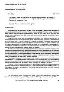
5 Re nement Rules In this section, we de ne some re nement rules that can transform a HLTPN into an implementation that is guaranteed to be correct by construction. The rules are de ned for a well-known subclass of HLTPNs: Merlin and Farber nets (MF nets) [Merlin&76]. An MF net is a HLTPN with strong time semantics, where time-functions associate each enabling tuple with an interval. Such interval can be described as a pair of constant values, called a Static Firing Interval, that represents the set of possible ring times, relative to the enabling time. The nets in Figures 1 and 3, with STS, may be easily rewritten as MF nets. Hereafter, we denote the time-functions as pair of constants representing the Static Firing Interval; the pair is written within square brackets in the graphical representation of the net. The transformation rules we identi ed are listed below informally. Given a net NS the application of a rule produces a new net NI which is an implementation of NS . All rules have been proven to satisfy the de nition of implementation presented in the former section, i.e. a net obtained by applying one of the rules presented below is guaranteed to be a correct implementation of the starting net. For the sake of simplicity, in this report, we omit the details of the formal proofs.
Transition Sequencing
Figure 4 shows the transition sequencing re nement rule. This re nement rule replaces a transition t with the sequence of two transitions t01 , t02 and a place p (Figure 4). The rule can be applied if there are no transitions con icting with t (i.e. no transitions sharing some place of their preset with the places in the preset of t). The transition sequencing rule can be applied to transition t2 of Figure 1. The action representing the communication between the producer and the consumer is detailed in two actions representing the start and the end of the communication respectively (transitions t21 and t22 of Figure 5).
Place Splitting
Figure 6 shows the place splitting re nement rule. Place p is replaced by two places p01 and p02 with the same preset and postset of p. If place p is initially marked, so will be places p01 and p02 . Since no transition is transformed, the event transformation is empty. Place p5 in Figure 5, representing two tasks (producer and consumer) during the communication, may be re ned into two di�erent places (places p51 and p52 in Figure 7) representing the state of the two tasks involved in communication separately.
IPTES-PDM-54-V2.0
10
p1
pn
p2
t1’ (alfa1’, beta1’)
t (alfa,beta) pn+1
pn
p2
p1
pn+2
p
pn+m
t2’ (alfa2’, beta2’)
pn+m
pn+2
pn+1
Timing Contraints Event Transformation t1 62 Domain( )
�1 + � 2 = � 1 + 2 = 0
0
0
0
0
(t 2 ) = t1 0
Figure 4: Transition Sequencing rule. p2 (ready for elaboration) p1 (ready for acquisition) t22 (end comm.) p5 (comm. in progress)
t3 (elaboration)
t1 (acquisition) t21 (start comm.) p3 (ready for communication)
p4 (ready for communication)
Figure 5: Application of the transition sequencing rule for re ning the MF net of Figure 1. t1
t2
tn
t1
p1
tn+1
tn+2
t2
p2’
p1’
tn+m
tn+1
tn
tn+2
tn+m
Figure 6: Place Splitting rule. IPTES-PDM-54-V2.0
11
p2 (ready for elaboration) p1 (ready for acquisition) t22 (end comm.) p52
p51
t3 (elaboration)
t1 (acquisition) t21 (start comm.) p3 (ready for communication)
p4 (ready for communication)
Figure 7: Application of the place splitting rule for re ning the MF net of Figure 5.
t1
tn
t2
t1
p1’
p
tn+1
tn
t2
t
tn+m
tn+2 tn+i
p2’
t’n+1
t’n+m
t’n+2
t’n+i (alfa’n+i,beta’n+i)
Timing Contraints Event Transformation 8n < i � n + m : � + � i = �i 8n < i � n + m : (t i ) = ti t1 62 Domain( ) + i = i 0
0
0
0
0
0
Figure 8: Place Sequencing Rule.
IPTES-PDM-54-V2.0
12
p2 (ready for elaboration)
p1 (ready for acquisition)
t22 (end comm.) p512
t1 (acquisition)
p52
t51
t3 (elaboration)
p511
t21 (start comm.) p3 (ready for communication)
p4 (ready for communication)
Figure 9: Application of the place sequencing rule for re ning the MF net of Figure 7. p1
p2
pn
p1
t (alfa,beta)
pn+1
p2
t1’ (alfa1’,beta1’)
pn+2
pn+m
pn+1
pn
t2’ (alfa2’,beta2’)
pn+2
pn+m
Timing Contraints Event Transformation
�1=�2=� 1= 2= 0
0
0
0
(t 1 ) = t
(t 2 ) = t 0 0
Figure 10: Transition Splitting rule.
Place Sequencing
Figure 8 shows the place sequencing re nement rule. This rule establishes that a place
p and the transitions in its postset can be replaced by places p01, p02, transition t0 and a set of transitions ft0n+i g, each of which corresponds to a transition tn+i 2 p� . Place p51 of Figure 7, representing the producer during the communication, is re ned into two places (p511 and p512) and a transition (t51) in Figure 9 in order to model the action executed during the communication (the body of the rendezvous).
Transition Splitting
Figure 10 shows the transition splitting re nement rule; transition t is replaced by transitions t01 and t02 which have the same preset and postset as t and the same static ring time intervals. Transition t51 of Figure 9, that represents the body of a rendezvous, can be further re ned into two transitions (t511 and t512) representing two alternative actions (e.g. an
IPTES-PDM-54-V2.0
13
p2 (ready for elaboration)
p1 (ready for acquisition)
t22 (end comm.) p512
p52
t512
t511
t1 (acquisition)
t3 (elaboration)
p511
t21 (start comm.) p3 (ready for communication)
p4 (ready for communication)
Figure 11: Application of the transition splitting rule for re ning the MF net of Figure 9. p1
p2
pn
p1
t (alfa,beta)
pn+1
p2
pn
t’ (alfa’,beta’)
pn+2
pn+m
pn+1
pn+2
pn+m
Timing Contraints Event Transformation
��� � � 0
0
(t ) = t 0
Figure 12: Firing Time Reduction rule. \if" inside the body of the rendezvous), as shown in Figure 11.
Firing Times Reduction
Given a net N the ring time reduction re nement rule, shown in Figure 12, consists of substituting a generic transition t of N with a new transition t0 having a more restricted static ring interval. The application of this rule to transitions t511 and t512 of Figure 11 reduces their ring time interval. It can be used to represent the fact that the two transitions (t511, t512) correspond to actions with di�erent timing (e.g. tft511 (p511) = [0; 0:7], tft512 (p511) = [0:6; 0:9])
Iteration
The iteration re nement rule, shown in Figure 13, consists of substituting a transition t with a set of transitions and places that represent the execution of the action modeled IPTES-PDM-54-V2.0
14
p1
p1
p2
p2
pn
t1’ (alfa1’,beta1’)
pn
t2’ (epsilon’,epsilon’) t (alfa,beta) t3’ (delta’,delta’)
pn+1
pn+2
pn+m
t4’ (alfa2’,beta2’)
t’5 (0,0)
pn+1
pn+2
pn+m
Timing Contraints Event Transformation
� + � + 1 + 2 = t1 ; t2; t3; t4 62 Domain( ) � + �1 = �
(t 5 ) = t � >0 0
0
0
0
0
0
0
0
0
0
0
0
Figure 13: Iteration Rule. by transition t, as an action that may be repeated several times in a cycle. The structure of the resulting net guarantees an upper bound to the number of cycles so that the total execution time is not greater than the execution time of the original transition t. The HLTPN in Figure 3 can be obtained from the net in Figure 11 applying the ring time reduction rule followed by the iteration rule applied to transition t3 . The idea behind this example is that the consumer's behavior is described by two tasks: a time-out controlling the timing and an iteration executing the computation. The net in Figure 3 is a correct re nement of the net of Figure 1, by construction, Thus it satis es the time properties of the net in Figure 1, since it is obtained by applications of the property preserving re nement rules described in this section.
6 The Prototype A rst prototype that automatically applies the re nement rules to HLTPNs speci cation has been implemented. The prototype uses the services of Cabernet7 ([Pezze&92]). The embedding in Cabernet provides several advantages:
� the possibility of reusing important parts (e.g. graphical interface and data and �
7
management facilities), that are needed to provide reasonable access to the prototype, but are not strictly part of it. the possibility of reusing existing technology and expertises of PDM. After the reductions in man e�ort moved from this task to more urgent tasks, the design,
Cabernet is part of the IPTES background
IPTES-PDM-54-V2.0
15
�
implementation, testing and documentation of the toolset has been completed with an e�ort of 6 man months. Only the heavy reuse of technology and expertises made possible to realize an interesting prototype with such a small e�ort. the integration with other advanced tools, and in particular with the analysis prototype, that has also been integrated in Cabernet for similar reasons. In this way the two prototypes (analyser and hierarchy manager) could be used for experimental veri cation of the bene ts of the two di�erent technologies for the analysis of large speci cations.
The integration with Cabernet has no big e�ects on the overall project. The hierarchical decomposition toolset comprises two basic tools: a re nement tool and a navigation tool. The re nement tool allows the end-user to apply the re nement rules described in this document to a HLTPN. It rst checks the selected element for compatibility with the selected rule (e.g. it checks that the transition sequencing rule is applied to a transition). It also checks that the net to which the rule is applied is an MF net, in fact the rules described in this document and implemented by the re nement toolset can be applied only to MF nets. It then acquires, if needed, the new time functions from the user; it checks for their validity with respect to the time functions associated to the transitions in the original HLTPN; it produces the time functions that can be automatically derived, and, nally, produces the new HLTPN. We report here, for each re nement rule, the input that the end-user must provide, and the controls and computations performed by the tool:
Transition sequencing rule: allows the end-user to select the time function associ-
ated with one of the two produced transition. The lowest and the greatest ring time speci ed by the end-user must be no higher than the lowest and the greatest ring time of the re ned transition respectively. If these requirements are veri ed, the tool derives the time function of the other produced transition. Otherwise, it refuses to apply the rule and does not generate a re ned HLTPN. Place splitting rule: no datum is required from the end-user. The tool automatically generates the new time functions associated with the transitions in the postset of the re ned places. Place sequencing rule: the end-user must provide the time function associated with the newly produced transition. The tool checks that the lowest and the greatest ring time of the new transition are not greater than any of the lowest and greatest ring times associated with the transitions in the postset of the re ned place respectively. It then generates the new time functions for the transitions in the postset of the re ned place. Transition splitting rule: no datum is required from the end user. The tool automatically computes the time functions associated with the new transitions. Firing time reduction rule: the end-user must provide the new time function. the toolset controls whether it is comprised in the old time function or not. If not, the re nement step is refused as incorrect. Iteration rule: such rule has not been implemented yet in the current prototype. IPTES-PDM-54-V2.0
16
Figure 14: The cabernet window The navigation tool allows the end-user to access the di�erent level of re nement of the speci cation. The current version supports a total order of re nement levels: only the most re ned level can be further re ned. In the reminder of this section we present a few guidelines to simplify the access to the toolset. Here, we also give a few suggestion on how to use Cabernet for creating a net. The use of Cabernet is straightforward. The end-user is referred to the Cabernet documentation available with Cabernet for a detailed introduction on the tool. It can also refer to [Bellettini&93] (the documentation of the analysis toolset) for a more general, yet incomplete introduction to the use of Cabernet. The reader is strongly suggested to use the reminder of this section as a guide while practising with the toolset.
User manual
The hierarchical decomposition toolset is fully integrated in Cabernet that provides graphical display and editing facilities. Cabernet can be launched on an X server, using the command cabernet. The gnu C++ compiler required for the use of the HLTPN executor and animator is not strictly necessary for running the hierarchical decomposition toolset. The Cabernet interface is the Xwindows shown in Figure 14. HLTPNs can be drawn in the main window by using the buttons on the upper left IPTES-PDM-54-V2.0
17
hand side. Each bottom must be selected before clicking on the canvas. The buttons examined from top left to bottom right allow:
� to select one or more elements (places, transitions, arcs). The rst element can � � � � �
be selected using the leftmost button, further elements can be selected using the rightmost button. Selected elements can be used later for applying further actions, e.g. move. to move the selected elements. Once selected the move button (indicated with a little hand) any element can be moved using the leftmost button of the mouse. The current set of selected elements can be moved using the rightmost button of the mouse. Elements are moved clicking on them an dragging the mouse before releasing the button. to create a new place. Clicking on the canvas produces a new place associated with default values. to create a new transition. Clicking on the canvas produces a new transition associated with default values. to create a new arc. Clicking on a node (either a place or a transition) and then on a second node (a transition, if the rst one was a place, a place otherwise) creates an arc between the two nodes. Intermediate clicking introduce bending points in the new arc. to add tokens. Clicking on a place adds a token in such a place.
Each created element can be modi ed by selecting the selection button and double clicking on the element to be modi ed. A suitable mask appears. The mask popped up when double clicking on a transition is shown in Figure 15. For running the hierarchical decomposition toolset only few attributes related to transitions are interesting:
Semantics, strong time semantics must be selected Static min time, indicating the lowest ring time for the transition; it must be the
keyword enab (indicating the maximum among the time-stamps associated with the enabling tuple) followed by a + and a constant (it can be integer or real). Static max time, indicating the highest ring time for the transition; same syntax as EFT. The constant should be no less than the constant used for the EFT eld, to make the net meaningful. Additional editing commands, including cut, paste, and modify are available under menu edit. Nets created with the graphical editor can be saved and loaded using the self explanatory items under menu le. The re nement tool is accessible via menu re ne, shown in Figure 16. The end -user must rst select the node (either a transition or a place) to which the re nement rule has to be applied using button select from the buttons on the left hand side described above, and then one of the re nement rules listed under menu re ne. If the net is not an MF net or the selected rule does not apply to the selected element the re nement is aborted and suitable messages are popped up. Otherwise the system asks the end-user IPTES-PDM-54-V2.0
18
Figure 15: The mask popped up when double clicking on a transition
IPTES-PDM-54-V2.0
19
Figure 16: Menu re ne
Figure 17: The mask asking the end-user for the time function of one of the transitions generated by the transition sequencing re nement rule. for further details, if needed, through a suitable mask. Items \Transition Cycle", \User Choice", and \Check" are not implemented in the current version. As an example, the mask asking for the time function for the transition sequencing re nement rule is shown in Figure 17. Finally the new HLTPN is shown on the canvas window. The navigation tool can be invoked through the menu Hierarchy, shown in Figure 18. It allows the visualization of the next or the former level in the hierarchy. Suitable messages are popped up if the end-user attempts to go beyond the rst or the last level. Menu Hierarchy also allows a hierarchy to be saved. It di�ers from the corresponding command available under menu le because it causes the whole hierarchy information to be save and not only the current net.
Figure 18: Menu hierarchy
IPTES-PDM-54-V2.0
20
The reader is referred to the Cabernet documentation for further commands available, but not strictly needed for using the hierarchical decomposition toolset described in this document.
7 Conclusions Speci cations may contain aws. If such aws remain undetected, they can propagate down to design, implementation and even to the delivered systems. An important bene t of formal speci cations is that they provide conceptual means for early validation, based on various kinds of analysis techniques. Unfortunately for most speci cation formalisms having high expressive power, analysis procedures either cannot be performed mechanically to check meaningful properties, or their computational cost is too high. High complexity inhibits scalability of analysis techniques from simple examples to realistic, complex cases. In this report we discussed these issues in the context of operational speci cations of real-time systems given in terms of HLTPNs. We categorized the properties we wish to prove to validate speci cations as bounded invariance and bounded response. We discussed how to analyze these properties in the case of speci cations given through levels of abstractions. We de ned the concept of correct re nement of a HLTPN, and we were able to show that interesting timing properties are preserved by correct re nements. We also introduced constructive transformation rules which can be proven to yield correct re nements. Currently, we are using the re nement concepts de ned in this report for the incremental analysis of real size systems, using the prototype developed at Politecnico di Milano. From this work, we hope to be able to identify new useful re nement rules to be de ned. We are also working on e�cient techniques for proving that re nement rules de ned ad-hoc by the end-users are correct re nements. Finally, we are trying to identify new implementation relations preserving di�erent set of properties. The rules de ned in this report are not shown to directly correspond to the re nements possible at the SA/SD-RT level. Investigating these relations has not been possible due to lack of time. At a rst look, it seems like some SA/SD-RT hierarchical re nements rule can nd a correspondence with the rules presented here, some other cannot. Whether the set of rules de ned here can be extended to completely match the SA/SD-RT hierarchical decomposition rules or not is left to further investigation. The authors feel like some SA/SD-RT hierarchical decomposition rules cannot be matched at all due to their intrinsic informality that cannot match a rigorous formal framework as de ned in this report.
8 References [Aizikowitz90]
Aizikowitz J. Designing distributed services using re nements mappings. PhD thesis, Department of Computer Science, Cornell University, 1990.
IPTES-PDM-54-V2.0
21
[Bellettini&93]
Carlo Bellettini, Miguel Felder, Mauro Pezz�e. A tool for analysing High-Level Timed Petri Nets. Technical Report, Politecnico di Milano, July 1993. IPTES Doc.id.: IPTES-PDM-41-V2.0.
[Damm&90]
Damm W., Dohmen G., Volker G., Josko B. Modular veri cation of Petri nets, the temporal logic approach. In Proceedings of CAV 1990, 1990. LNCS vol. 430.
[Felder&92]
Miguel Felder, Carlo Ghezzi, Mauro Pezz�e. HLTPN Kernel Model. Technical Report, Politecnico di Milano, July 1992. IPTES Doc.id.: IPTES-PDM-6-V3.0.
[Ghezzi&91]
Carlo Ghezzi, Sandro Morasca, Mauro Pezz�e. Timing Analysis of Time Basic Nets. Technical Report, Politecnico di Milano, July 1992. IPTES Doc.id.: IPTES-PDM-29-V1.0.
[Glabbeek&90]
Glabbeek R., Goltz U. Re nement of actions in causality based models. In Proceedings of CAV 1990, 1990. LNCS vol. 430.
[Huber&89]
Peter Huber and Kurt Jensen and Robert Shapiro. Hierarchies in Coloured Petri Nets. 10th International Conference on Application and theory of Petri Nets, June 1989.
[Merlin&76]
P.M. Merlin, D.J. Farber. Recoverability of Communication Protocols { Implications of a Theoretical Study. IEEE Transactions on Communications, September 1976.
[Pezze&92]
Carlo Ghezzi, Mauro Pezz�e. Cabernet: an Environment for the Speci cation and Veri cation of Real-Time Systems. Proceedings of the DECUS Conference, September 1992. Cannes.
[Vogler90]
Vogler W. Failures semantics based on interval semiwords is a congruence for re nement. In Proceedings of STACS 1990, 1990. LNCS vol. 415.
[Ward&85]
P.T. Ward and S.J. Mellor. Structured Development for Real-Time Systems. Volume 1-3, Yourdon Press, New York, 1985-1986.
IPTES-PDM-54-V2.0
End of Document
22