Distributed Spectrum-Efficient Routing Algorithms in Wireless Networks

1

Distributed Spectrum-Efficient Routing Algorithms in Wireless Networks Deqiang Chen, Martin Haenggi, Senior Member, IEEE J. Nicholas Laneman, Member, IEEE

Abstract This paper applies spectral efficiency as a performance measure for routing schemes and considers how to obtain a good route in a wireless network. The objective for this study is to combine different perspectives from networking and information theory in the design of routing schemes. The problem of finding the optimum route with the maximum spectral efficiency is difficult to solve in a distributed fashion. Motivated by an information-theoretic analysis, this paper proposes two suboptimal alternatives, namely, the approximately-ideal-path routing (AIPR) scheme and the distributed spectrum-efficient routing (DSER) scheme. AIPR finds a path to approximate an optimum regular path and requires location information. DSER is more amenable to distributed implementations based on Bellman-Ford or Dijkstra’s algorithms. The spectral efficiencies of AIPR and DSER for random networks approach that of nearest-neighbor routing in the low signal-to-noise ratio (SNR) regime and that of single-hop routing in the high SNR regime. In the moderate SNR regime, the spectral efficiency of DSER is up to twice that of nearest-neighbor or single-hop routing.

I. BACKGROUND

AND

M OTIVATION

As wireless communications are extended beyond the last hop of networks, a better understanding of wireless relaying (including routing as a special case) is needed to deploy efficient multihop wireless networks. Research from different perspectives, e.g., networking and information theory, yields in different relaying paradigms for wireless networks [1]–[7]. The goal of this This work has been supported in part by NSF Grants CCF05-15012 and CNS06-26595. Deqiang Chen, Martin Haenggi and J. Nicholas Laneman are with Department of Electrical Engineering, University of Notre Dame, Notre Dame, IN 46556, Email: {dchen2, mhaenggi, jnl}@nd.edu Parts of the material in this paper have been presented at CISS 2007. September 13, 2007

DRAFT

2

paper is to study the wireless routing problem combining networking and information-theoretic perspectives. The study of wireless networks using information theory [1]–[4] has led to several relaying protocols that are asymptotically order-optimal as the number of nodes goes to infinity. However, all practical networks have a finite number of terminals. Furthermore, relaying protocols derived from information theory often involve complicated multiuser coding techniques, such as block-Markov coding and successive interference cancellation, which are often too complex to implement in practical systems. Moreover, information-theoretic relaying strategies may not be easily implementable in a distributed manner. The gap between information-theoretic analyses and practical implementations has inspired us to study networks with a finite number of nodes with an emphasis on the distributed implementation aspects of our routing schemes. On the other hand, previous work on routing within the networking community, e.g., [6], [7], mainly studies how to design new routing metrics to improve the throughput, and how to modify existing routing protocols to incorporate new metrics. These models are often built on link-level abstractions of the network without fully considering the impact of the physical layer. There is little if any discussion about the fundamental performance limits, such as Shannon capacity or spectral efficiency. In contrast to these works, this paper studies the influence of different routing schemes on spectral efficiency and designs distributed routing schemes based on insights from an information-theoretic analysis. The work in [8]–[10] provides important guidelines for designing spectrum-efficient networks. Assuming a one-dimensional linear network, [8]–[10] show that there is an optimum number of hops in terms of maximizing end-to-end spectral efficiency. The results challenge the purely signal-to-noise ratio (SNR) guided traditional wireless routing paradigm of “the more hops the better”. However, [8]–[10] assume that the number of relays and their locations are design parameters. In practice, the network geometry changes as the network operates and evolves; thus, neither the number of available relay nodes nor their locations between a source and destination are design parameters. Therefore, this paper considers choosing a route in a network comprised of an arbitrary number of randomly located nodes. The remainder of the paper is organized as follows. Section II describes the system model and assumptions. Section III formulates the problems of finding a route with the maximum spectral efficiency assuming both the optimal bandwidth allocation and the equal bandwidth allocation. September 13, 2007

DRAFT

3

Since bandwidth allocation requires exchange of at least some global information, most of the paper focuses on providing solutions for the case of equal bandwidth sharing. Specifically, Section IV proposes approximately-ideal-path routing (AIPR), a location-assisted routing scheme, and Section V proposes distributed spectrum-efficient routing (DSER) scheme as another nearoptimum solution. The spectral efficiency of AIPR and DSER closely follows the optimal spectral efficiency. Furthermore, DSER can be implemented with standard distributed algorithms that are guaranteed to converge and generate loop-free paths. Section VI discusses the applications of AIPR and DSER in interference-limited networks and the connections between DSER and other well-known routing schemes. Section VII presents simulation results, and Section VIII concludes the paper. II. S YSTEM M ODEL A. Network Model For simplicity, we only consider routing for one source-destination pair and limit our study to single-path routing. Also we do not allow the links to exploit cooperative diversity, e.g., [11], [12]. One typical assumption in networks is that there is no link between two nodes if the signal quality is below certain thresholds [1], [6], [7]. However, from an information-theoretic perspective, two nodes can always communicate with a sufficiently low rate. Therefore, in this paper we assume any two nodes in the network can directly communicate. We represent the nodes in a network and the possible transmissions between nodes by a complete graph G = (V, E), where V represents the set of nodes in the network and E represents the set of edges (links). In general, nodes are arbitrarily located. For each link e ∈ E, we use t(e) to represent the transmit end of the link and r(e) to represent the receive end. A path L from node s to node d, s 6= d, consists of an ordered sequence of unique links l1 , l2 , l3 , ..., ln ∈ E that satisfies the following: for each 1 ≤ k ≤ n − 1, r(lk ) = t(lk+1 ); t(l1 ) = s; and r(ln ) = d. We also denote the source and destination of a given path L as t(L) = t(l1 ) and r(L) = r(ln ), respectively. The length of the path |L| is the number of links or hops in the path.

September 13, 2007

DRAFT

4

B. Channel Model We use a standard path-loss model, i.e., the path-loss factor from node i to node j, i, j ∈ V, is given by Gi,j = c[max(Di,j , Df )]−α ,

(1)

where Di,j is the Euclidean distance between node i and j, Df is the far-field distance [13], α is the path loss exponent (typically taking values between 2 and 4), and c is a constant. For most practical scenarios, Di,j is much larger than Df ; thus, (1) can be approximated as −α Gi,j ≈ cDi,j .

(2)

For simplicity of presentation, we mainly use (2). We can also express Gi,j as Gl where l ∈ E, t(l) = i, r(l) = j. In this paper, after appropriately normalizing the transmission power, which is sufficient for relative comparison, we will assume that c = 1. The received signal is further corrupted by additive white Gaussian noise (AWGN) with a normalized one-sided power spectral density N0 , which is assumed to be the same for all receivers. We consider the setting in which all transmit devices are constrained by the same symbolwise average transmit power P and assume all devices transmit with power P when transmitting. This assumption is justified by the fact that, for low-power transceivers, local oscillators and bias circuitry dominate energy consumption [14]. Moreover, the radio frequency (RF) power amplifier (PA) should mostly operate close to its saturated power for the most energy efficient operation, as this is when the power added efficiency (PAE) is largest [15]. Another observation in support of this assumption is that nodes in wireless mesh networks are mostly immobile and connected with abundant power supplies. We further assume that the network is supplied with a finite bandwidth B (Hz) and define the network SNR as ρ :=

P . N0 B

(3)

For link l ∈ E, we define the SNR on link l as ρl = ρGl ,

(4)

where Gl is the path-loss factor along the link. We define the spectral efficiency RL for a path L as the bandwidth-normalized end-to-end rate, i.e., RL = CL /B b/s/Hz, where CL is the end-to-end achievable rate in bits per second given a bandwidth constraint B along the path L [8]. September 13, 2007

DRAFT

5

C. Scheduling In general, optimum scheduling in networks is NP-hard [16]. To avoid the difficulty of jointly optimizing routing and scheduling, we first assume the network operates with time division multiple access (TDMA) without spatial reuse, i.e., each node transmits in its own unique time slot. For a network with spatial reuse of bandwidth, it is important to design the medium access control (MAC) layer judiciously to mitigate interference. In this case, the interference stays approximately constant over time, and our framework is directly applicable by adding the interference to the noise. In Section VI-A, we will discuss extensions of our routing schemes to a simple scheduling scheme that allows for some spatial reuse. III. O PTIMAL ROUTING This section discusses selection of routing paths that maximize the end-to-end spectral efficiency. The resulting optimization problem and its solution depend on whether the bandwidth or time slots can be optimally allocated across links. Given optimum bandwidth allocation among links, [9] shows that the maximum spectral efficiency along a route L is 1

. 1 l∈L log(1+ρl )

P

(5)

Since the denominator of (5) is additive, we can use Bellman-Ford or Dijkstra’s algorithms with a link metric of 1/ log(1 + ρl ) to find the route that maximizes the spectral efficiency by P minimizing l (1/ log(1 + ρl )) [9]. We refer to such a routing scheme as optimal routing with

bandwidth optimization (ORBO). Although ORBO can be performed in a distributed fashion, allocating bandwidth requires propagating the value of (5) backwards to the nodes on the route [9]. As we will see, ORBO is most beneficial in the low SNR regime, where the power spent in distributing this knowledge may not be neglected. Another concern about bandwidth optimization is the issue of fairness, as one node with a larger share of the bandwidth might spend more energy than other nodes with a smaller share of the bandwidth. For these reasons, the rest of the paper focuses on the case of equal bandwidth sharing. Under the constraint of equal bandwidth sharing, the end-to-end spectral efficiency of a given path L is [17], [18] RL = min l∈L

September 13, 2007

1 log(1 + ρl ), |L|

(6) DRAFT

6

where the factor 1/|L| results from the sharing of bandwidth among relay links. For a path L, the signal quality is reflected by the worst link SNR ρ∗L = minl∈L ρl , and the bandwidth use is characterized by inverse of the number of hops |L|. The spectral efficiency (6) increases as ρ∗L increases or |L| decreases. However, for routes connecting a given source and destination, if the number of links |L| increases (or decreases), there are more (or less) relay nodes and ρ∗L is more likely to increase (or decrease) due to shorter (longer) inter-relay distances. This trade-off can be seen by comparing the nearest-neighbor route and the single-hop route (the source directly transmits to the destination) in a linear network. Among all routes connecting a given source and destination, the nearest-neighbor route has the largest ρ∗L but also the largest |L|. On the other hand, single-hop has the smallest ρ∗L , but also has the smallest |L|. Therefore, there is a trade-off between physical layer parameters, i.e., signal quality and bandwidth use, in selection of routes. The optimal routing scheme takes this trade-off into account by providing a solution to the optimization problem max

L:t(L)=s,r(L)=d

min l∈L

1 log(1 + ρl ), |L|

(7)

where nodes s and d form the desired source-destination pair. Unfortunately, generalized Bellman-Ford and Dijkstra’s algorithms cannot be used to solve (7), because the routing metric (6) is neither isotonic nor monotone [19], [20]. In general, the computation of the spectral efficiency by (6) requires global information about a path. Therefore, the problem in (7) does not exhibit the optimal substructure that is necessary for the use of dynamic programming methods [21]. The solution to (7) can in principle be obtained by an exhaustive search method. However, for a network with n relays, there are at least 2n−1 different reasonable routes connecting the source and destination. This exponential growth makes exhaustive search unrealistic in practice if the network has a moderate to large number of relay nodes. More importantly, an exhaustive search method is not amenable to distributed implementation. In the following, Section IV and Section V provide two suboptimal solutions to (7) that are more amenable to distributed implementation. IV. A PPROXIMATELY I DEAL PATH ROUTING (AIPR) The motivation for our first scheme is to approximate the ideal regular path; we thus refer to this routing scheme as the approximately ideal path routing (AIPR) scheme. AIPR directly September 13, 2007

DRAFT

7

utilizes the Euclidean distance to select relays, and thus differs from the nth -nearest-neighbor routing schemes [22]. For a given source and destination, [8] suggests that in a regular linear network there is an optimum number of hops nopt . More specifically, the number of links in an optimal regular linear network satisfies [8] nopt R ≈

α + W(−αe−α ) , ln 2

(8)

where R is the path spectral efficiency, and W(·) is the principal branch of the Lambert W function [23]. Combining (2), (6) and (8), we obtain the number of hops in an optimal regular linear network given the network SNR ρ:  !1/α  [α+W(−αe−α )]/ ln 2 2 −1  , nopt ≈  ρ

(9)

+

where [·]+ rounds the operand to the nearest positive integer. Assuming that the distance between the source and destination Ds,d and the network SNR are known, the optimum inter-relay distance

Dhop is Dhop = Ds,d/nopt .

(10)

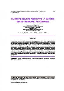
Thus, an optimum regular linear network connecting node s and d consists of nopt hops with a per-hop distance Dhop . The above discussion applies to networks in which both the number and locations of relays can be designed. However, such a regular linear path with an ideal inter-relay distance most likely will not exist in more general network scenarios. As an alternative, we propose the procedure as shown in Algorithm 1 to find a path approximating this ideal path given that location information is available. The basic idea is demonstrated in Fig. 1. Starting from the source, we look for a relay node that lies within a distance Dhop and in the right direction to the destination. If no such node is available, Algorithm 1 increases the per-hop distance Dhop by δ. After the source chooses its relay node, the source passes the value of Dhop to the relay, which repeats the process of finding its next relay node and passing the value of Dhop until the destination is reached. The source is assumed to know Ds,d in order to compute the initial value of Dhop . A transmit node is assumed to know the destination location in order to proceed in the right direction and to know location information for at least neighboring nodes. To prevent the path from going in the wrong direction in the two-dimensional plane [22], the search for the relay is limited inside a September 13, 2007

DRAFT

8

sector originated from the transmitter with a radius Dhop and with an angle φ/2, 0 ≤ φ ≤ π of the axis to the destination as suggested in [22]. Algorithm 1 AIPR 1: {Node s and d denotes the source and destination respectively; P ath[0...N] is a sufficiently large array with initial value NULL and will contain the path; sect(a, b, r, φ/2) denotes the sector originated from node a, with a radius r and an angle φ/2 of the axis from the node a to b; δ is the given step in increasing the inter-relay distance D.}

4:

calculate Dhop based on (10); sˆ = s; dˆ = NULL; P ath[0] = s; n = 0; D = Dhop ; while dˆ 6= d do

5:

if No relay node lies in sect(ˆ s, d, D, φ/2) then

2: 3:

6:

D = D + δ;

8:

else if node d lies in sect(ˆ s, d, D, φ/2) then ˆ dˆ = d; P ath[n++] = d;

9:

else

7:

10:

choose the relay node in sect(ˆ s, d, D, φ/2) with the largest distance from node sˆ, denote ˆ it as node dˆ and P ath[n++] = d;.

11:

end if

12:

end while

In AIPR, a transmit node is assumed to know the destination and neighboring nodes’ location information. In the following section, we propose an alternative routing scheme that does not rely on location information. V. D ISTRIBUTED S PECTRUM -E FFICIENT ROUTING (DSER) The motivation for our second routing scheme, namely, the distributed spectrum-efficient routing (DSER) scheme, is to balance the trade-off between the power efficiency and bandwidth efficiency, thus improving the spectral efficiency. More specifically, the discussion in Section III suggests that longer per-hop distances might result in power inefficiency, and shorter per-hop distances might result in bandwidth inefficiency. Thus, there is both a penalty and a reward, in

September 13, 2007

DRAFT

9

terms of spectral efficiency, with the addition of intermediate relay links. This motivates us to solve the following problem for a spectrum-efficient route: X β min 1+ , L:t(L)=s,r(L)=d ρl l∈L

(11)

where, as before, nodes s and d form the desired source-destination pair, and β ≥ 0, referred to as the routing coefficient, is a parameter that can be designed. Intuitively, the additive constant 1 represents the penalty on bandwidth efficiency for additional hops; the factor 1/ρl characterizes SNR gains by using links with short distances; and the parameter β weights the impact of power

and bandwidth. A routing algorithm can use 1 + β/ρl as the link metric and use distributed Bellman-Ford or Dijkstra’s algorithms to solve (11). As we will see, this routing scheme can offer significant gains in spectral efficiency compared to nearest-neighbor routing or single-hop. The DSER scheme does not depend on the particular path-loss model in (2). In practice, the link SNR can be directly measured by received signal strength indicators (RSSI) available on most devices and fed back to the transmitters. A. Values of the Routing Coefficient To determine the routing coefficient β, we note that (9) provides the optimum number of hops nopt for the design of a regular linear network. Now, if we assume that DSER is used to design a regular linear network connecting a particular source-destination pair with a unit distance and SNR ρ, the objective function to be minimized becomes   β|L|−α f (|L|) = |L| 1 + . ρ

(12)

We relax |L| as a real number, differentiate (12) with respect to |L| and set df (|L|)/d|L| = 0 to obtain an expression for the optimum number of links |L|opt . By setting |L|opt = nopt , we obtain eα+W(−αe ) − 1 β= . α−1 −α

(13)

The routing coefficient determined by (13) is independent of the network SNR and can be determined by the channel model. Furthermore, in the range 1 < α ≤ 5, (13) can be very accurately approximated as β ≈ 2α .

September 13, 2007

(14)

DRAFT

10

In Section VII we present simulation results to show that DSER performs quite well using these approximations. It can be observed from (14) that the value of routing coefficient increases drastically as the path loss exponent increases. This suggests that the SNR gain of shorter hops is assigned a higher weight as the path loss exponent increases. As a result, DSER favors a route with a shorter per-hop distance to combat the path loss when the path loss exponent is large. We note that (13) is developed essentially assuming there are an infinite number of nodes and a continuum of locations from which to choose. Moreover, our derivation has not fully taken into account the effect of modulation, coding, queueing, and so forth. Therefore, for an arbitrary network with a finite number of nodes and practical communication schemes, the value of β can be further tuned, e.g., for a specific network geometry, network SNR, modulation format, and so forth, to improve the spectral efficiency of the DSER scheme. B. Properties From (11), it is straightforward to see that for a given network, the route generated by DSER depends on the link SNRs. In the high SNR regime, β/ρl ≪ 1, i.e., the cost of sharing bandwidth among many links outweighs the SNR gains of shorter inter-relay distances. Thus, the DSER route will approach single-hop between the source and destination in this regime. In the low SNR regime or the high path loss exponent regime, β/ρl ≫ 1, i.e., the SNR gains of shorter links outweigh the cost of sharing bandwidth. In such scenarios, the performance of DSER will approach that of nearest-neighbor routing. The discussion here agrees with simulation results we will present in Section VII. For the DSER scheme, the weight of a path L is W (L) =

P

l∈L

1 + β/ρl . For any paths

L1 , L2 , L3 , if W (L1 ) < W (L2 ), we have both W (L1 ⊕ L3 ) < W (L2 ⊕ L3 ) and W (L3 ⊕ L1 ) < W (L3 ⊕ L2 ), where L1 ⊕ L2 denotes the concatenation of two paths L1 and L2 . Thus, the DSER metric is strictly isotonic [19]. Moreover, for any paths L1 , L2 , we have W (L1 ) ≤ W (L1 ⊕L2 ) if t(L2 ) = r(L1 ), i.e., the DSER metric is monotone [20]. It has been shown [19] that for link-state routing protocols, isotonicity of the path weight function is a necessary and sufficient condition for a generalized Dijkstra’s algorithm to yield optimal paths. If the path weight function satisfies strict isotonicity, forwarding decisions can be based only on independent local computation, and the resulting path is loop free. For path vector routing protocols, monotonicity of the path weight function implies protocol convergence in every network, and isotonicity assures convergence of September 13, 2007

DRAFT

11

algorithms to optimal paths [20]. Therefore, the DSER scheme can be implemented in existing networks with link-state or path vector routing protocols. Also, the path metric of the DSER scheme is additive, meeting a standard assumption of most existing implementations of BellmanFord or Dijkstra’s algorithms [21]. Thus, DSER can be implemented on top of existing wireless network routing protocols such as DSR and AODV [5], [6]. By contrast, AIPR is not as easy to incorporate into existing routing protocols. However, as we will see, AIPR offers certain advantages in low SNR regimes, thus is a good alternative for routing in wireless sensor networks, where location information can be available to sensor nodes. VI. E XTENSIONS A. Spatial Reuse AIPR and DSER have so far been developed without taking into account the effect of spatial reuse of bandwidth, i.e., without considering interference. However, it is worth noting that the condition (8), which guides our design of AIPR and DSER, turns out to be equivalent to, up to a factor of 2, the condition for maximizing the intensity of transmission in an interference-limited network [24]. In the context of [24], nopt can be viewed as the number of orthogonal sub-bands and R as the required spectral efficiency on each link. As indicated in Section II, joint design of routing and scheduling can be difficult. For the purpose of illustrating that our routing schemes can benefit from spatial reuse, it suffices to consider a separate design approach: apply the routing scheme assuming no interference to obtain a route, and then apply a scheduling algorithm to the selected route. In particular, we consider modulo-K scheduling [8], also called K-phase TDMA [25]: two links li , lj ∈ L can use the same time slot if (i − j) mod K = 0 where

mod is the modulo operation. Note that we

assume the transmission is scheduled in the right order. The idea of modulo-K scheduling is to limit the co-channel interference while reusing wireless resources spatially. For each route, we choose an optimum K that maximizes the path spectral efficiency. Even though allowing nodes to transmit with different levels of power might improve the efficiency of networks via power control, we only consider the constant transmit power assumption as argued in Section II-B. Note that both modulo-K scheduling and the constant transmit power assumption are not optimal in general, but they suffice to show that spatial reuse can improve the spectral efficiency of the

September 13, 2007

DRAFT

12

DSER scheme. In Section VII, we present simulation results showing that at low SNR the spectral efficiency of DSER with modulo-K scheduling is larger than without spatial reuse. Note that once a path L is determined, the spectral efficiency of the path with a modulo-K scheduling is given by RL = min l∈L

1 log(1 + γl ), K

(15)

where K is the number of time slots needed for scheduling and γl is the signal-to-interferenceand-noise ratio (SINR) of link l ∈ L, i.e., γl =

ρl 1+

P

ρGt(li ),r(l)

,

(16)

{li :li ∈L,li 6=l,τ (li )=τ (l)}

with τ (l) denoting the time slot used by link l. B. Relation of DSER to Other Protocols

It turns out that DSER is related to several widely known routing metrics. As we will show in the sequel, by adjusting the routing coefficient β, the DSER metric specializes to the minimal hopcount or to the expected transmission count (ETX) routing metric. These connections demonstrate the robustness of DSER. When β = 0, DSER falls back to minimal hop-count routing. As demonstrated in [26], minimal hop-count routing is very robust and provides good performance when network devices are highly mobile. Thus, even though DSER is developed assuming a relatively static network, it can still apply to a highly mobile network by choosing β = 0. With proper choice of β, the DSER metric can also approximate the ETX routing metric [6], a well-known metric for improving the throughput of wireless networks. To illustrate, we consider a network with an independently identical distributed (i.i.d) block Rayleigh fading model for each channel. Signals also suffer path loss as described in Section II-B. The fading coefficients are complex Gaussian random variables with zero mean and unit variance. Each link l has a desired link data rate R and uses automatic repeat-request (ARQ) until the message is correctly received. Denoting the packet error rate for link l as Ple , the average number of transmissions for a packet on a link is 1/(1 − Ple ). To minimize the end-to-end delay, the ETX scheme proposed in [6] aims to minimize the expected total number of packet transmissions, i.e., X 1 min . e L:t(L)=s,r(L)=d 1 − P l l∈L September 13, 2007

(17)

DRAFT

13

In terms of diversity-multiplexing trade-off, [27] shows that the main error event causing packet losses is outage. Thus, we approximate the packet loss rate by the outage probability,  R  2 −1 e Pl = 1 − exp − . ρl

(18)

Substituting (18) into (17), and making use the approximation ex ≈ 1 + x for small x, i.e., small R or large ρl , (17) becomes min

L:t(L)=s,r(L)=d

which is the same as (11) with

X

1+

l∈L

2R − 1 , ρl

β = 2R − 1.

(19)

(20)

Thus, with a proper choice of β, the DSER metric approximates the ETX routing metric for fading channels at high SNR. Comparing (20) with (14), we note that for ETX in the fading channel, the per-link data rate R assumes the role that α held in (14). As the per-link data rate requirement R increases, β increases, suggesting that the SNR gain provided by a shorter per-hop distance becomes more important in guaranteeing reliability. VII. S IMULATION R ESULTS This section presents simulation results to compare spectral efficiencies of different routing schemes averaged over random network realizations. Our simulations focus on uniformly random networks. For a one-dimensional linear network, we assume the source and destination are located at coordinates (0, 0) and (1, 0), respectively, and the horizontal coordinates of intermediate relay nodes are independent random variables uniformly distributed between 0 and 1. For a twodimensional network, we assume the source and destination are located at (0, 0) and (1, 1), respectively. The horizontal and vertical coordinates of the potential relay nodes are independent random variables uniformly distributed between 0 and 1. To estimate average spectral efficiency over the ensemble of random networks, we take the mean over 104 network realizations. In our simulations, the boundaries of the 95% confidence interval are within ±2% of the average value, assuming the spectral efficiency of a routing scheme is Gaussian distributed. Thus, the confidence interval is sufficiently-small, allowing us to compare routing schemes using these simulation statistics.

September 13, 2007

DRAFT

14

We also assume a path-loss model described in (1), taking the path loss exponent α = 4 and the far-field distance Df = 10−3 unless specified otherwise. Motivated by the approximation β ≈ 2α in Section V, the routing coefficient is taken to be β = 16. As two examples, Fig. 2 and 3 show the average spectral efficiency of different routing schemes including nearest-neighbor routing, single-hop, AIPR, and DSER for uniformly random linear networks with 5 and 9 nodes, respectively. To see a wider dynamical range around the low SNR regimes, the horizontal coordinate is taken as Eb /N0 , i.e., the ratio between the SNR and the average spectral efficiency. In Fig. 2 and 3, the optimal spectral efficiency is obtained by an exhaustive search method and is provided as a reference. It is clear that the performance of single-hop only approaches the optimum performance in the high SNR regime and suffers from a significant loss in spectral efficiency in the low SNR regime. The performance of nearestneighbor routing approaches the optimal performance in the low SNR regime, but degrades in the high SNR regime due to its inefficient use of bandwidth. By contrast, one can observe that the curves of the DSER scheme track the optimal curves throughout the whole SNR regime. In particular, in the moderate SNR regime, DSER offers significant gains in spectral efficiency relative to AIPR, nearest-neighbor routing, and single-hop. In particular, when Eb /N0 is around 0 dB, the spectral efficiency of the DSER scheme is twice as large as those of nearest-neighbor routing and single-hop. Thus, networks can benefit significantly in spectral efficiency from the use of DSER. DSER exhibits a drastic transition in performance around Eb /N0 ≈ 5dB. This is mainly due to the round-off error in (9). In random networks, AIPR suffers from a significant performance loss in the moderate SNR regime because it is difficult to find a regular linear path. However, AIPR performs reasonably well in either the low SNR or the high SNR regimes in our simulation. This is because at low SNR, AIPR degenerates into nearest-neighbor routing. Hence, the impact of path irregularity at low SNR is not as serious as at moderate SNR. In the high SNR regime, AIPR degenerates to choosing the direct link from the source to destination, which is the optimum route. We stress that our simulation does not fully consider the impact of fading, which might cause significant degradation in performance for AIPR. Fig. 4 shows the average spectral efficiencies of different routing schemes in a two-dimensional random network with 9 nodes. Note that the nearest-neighbor routing in Fig. 4 selects its nearest neighbor that lies within an angle φ/2 of the line from the source to destination, i.e., Strategy September 13, 2007

DRAFT

15

A in [22]. We choose φ = π/2. Compared to the case of one-dimensional random networks, the performance of DSER in two-dimensional random networks degrades in the low SNR regime. This could be explained by the fact that DSER does not require its relay node to lie within angle φ/2 of the line from source to destination, i.e., DSER does not require location information even in two-dimensional random networks. In contrast, both nearest-neighbor routing and AIPR require location information in two-dimensional networks. Other than this difference, most other observations from one-dimensional networks carry over to two-dimensional networks. Thus, in the remainder, we will only focus on the results from the one-dimensional case with the understanding that these observations carry over to the two-dimensional networks. Fig. 5 shows how DSER and AIPR adapt to different network SNRs, choosing different paths in a sample linear random network with 8 nodes. Note that based on (9), the optimum hop number of an optimum regular linear path for the network SNR of -20, 0 and 20dB is 8, 3 and 1, respectively. As shown in Fig. 5, DSER and AIPR choose paths with shorter hops when SNR is low. As the SNR increases, they tend to choose paths with longer inter-relay distance. Paths selected by AIPR and DSER are not necessarily the same. In particular, Fig. 5 shows that, relative to DSER, AIPR can choose a more balanced route at low SNR due to its utilization of location information. This observation is in line with our previous observation that AIPR can provide better performance at low SNR. Together with Fig. 3 – 4, Fig. 5 demonstrates that DSER and AIPR adapt to changes of the network SNR as we expected. Fig. 6 compares the performance of DSER with that of optimal routing with bandwidth optimization (ORBO). The spectral efficiency improves for ORBO mainly in the low SNR regime. However, as the network SNR increases, the benefit of bandwidth optimization decreases and eventually vanishes. This is because at high SNR, ORBO corresponds to single-hop, which is also the case for DSER. Fig. 7 show the average spectral efficiency as a function of the path-loss exponent for uniformly random linear networks with 9 nodes and network SNR of -40 and 20 dB. It might seem counterintuitive that the average spectral efficiency grows as the path-loss exponent increases. However, this is because our network SNR is end-to-end normalized SNR. Thus, as the path-loss exponent increases, the effective link SNRs on intermediate links increases as well. From Fig. 7, when the network SNR is high, the impact of different path loss exponent on routing schemes decreases. When the network SNR is small, relative to single-hop, routing schemes with multi-hop relaying September 13, 2007

DRAFT

16

benefit significantly from the high path loss exponent. Fig. 8 shows that even though DSER and AIPR are proposed assuming TDMA without spatial reuse, a modulo-K scheduling can further improve their performance at low SNR. Moreover, we observe that in the high SNR regime, there is not much to gain from spatial reuse, as single-hop between the source and destination is optimal. VIII. C ONCLUSION This paper studies end-to-end spectral efficiencies of different wireless routing schemes. This paper’s main contribution is to introduce two suboptimal solutions, namely, approximately ideal path routing (AIPR) and distributed spectrum-efficient routing (DSER), to the problem of finding routes with high spectral efficiency. AIPR is a location-assisted routing scheme. DSER can be based upon local link quality estimates, can be implemented using standard Bellman-Ford or Dijkstra’s algorithms, and can be integrated into existing network protocols. Furthermore, the performance of DSER and AIPR is close to that of nearest-neighbor routing and that of minimum hop-count routing in the low and high SNR regimes, respectively. In the moderate SNR regime, DSER provides significant gains in spectral efficiency compared with both nearest-neighbor routing and minimum hop-count routing. R EFERENCES [1] P. Gupta and P. Kumar, “The Capacity of Wireless Networks,” IEEE Trans. Inform. Theory, vol. 46, no. 2, pp. 388–404, 2000. [2] M. Gastpar and M. Vetterli, “On the Capacity of Large Gaussian Relay Networks,” IEEE Trans. Inform. Theory, vol. 51, no. 3, pp. 765–779, Mar. 2005. [3] G. Kramer, M. Gastpar, and P. Gupta, “Cooperative Strategies and Capacity Theorems for Relay Networks,” IEEE Trans. Inform. Theory, vol. 51, no. 9, pp. 3037–3063, Sep. 2005. [4] L.-L. Xie and P. Kumar, “A Network Information Theory for Wireless Communication: Scaling Laws and Optimal Operation,” IEEE Trans. Inform. Theory, vol. 50, no. 5, pp. 748–767, May 2004. [5] X. Hong, K. Xu, and M. Gerla, “Scalable Routing Protocols for Mobile Ad Hoc Networks,” IEEE Network Magazine, pp. 11–21, July/August 2002. [6] D. S. J. D. Couto, D. Aguayo, J. Bicket, and R. Morris, “A High-Throughput Path Metric for Multi-Hop Wireless Routing,” in Proc. ACM MOBICOM, 2003. [7] R. Draves, J. Padhye, and B. Zill, “Routing in Multi-radio, Multi-hop Wireless Mesh Networks,” in Proc. ACM MOBICOM, 2004.

September 13, 2007

DRAFT

17

[8] M. Sikora, J. N. Laneman, M. Haenggi, J. D. J. Costello, and T. E. Fuja, “Bandwidth- and Power-Efficient Routing in Linear Wireless Networks,” Joint Special Issue of IEEE Trans. Inform. Theory and IEEE Trans. Networking , vol. 52, no. 6, pp. 2624–2633, June 2006. ¨ Oyman and S. Sandhu, “A Shannon-Theoretic Perspective on Fading Multihop Networks,” in Proc. Conf. Inform. Sci. [9] O. and Syst. (CISS), 2006. [10] ——, “Non-Ergodic Power-Bandwidth Tradeoff in Linear Multi-hop Networks,” in Proc. IEEE Int. Symp. Information Theory (ISIT), 2006. [11] A. Sendonaris, E. Erkip, and B. Aazhang, “User Cooperation Diversity, Parts I & II,” vol. 15, no. 11, pp. 1927–1948, 2003. [12] J. N. Laneman, D. N. C. Tse, and G. W. Wornell, “ Cooperative Diversity in Wireless Networks: Efficient Protocols and Outage Behavior,” IEEE Trans. Inform. Theory, vol. 50, no. 12, pp. 3062–3080, December 2004. [13] T. Rappaport, Wireless Communications: Principles and Practice. Prentice Hall PTR, 2001. [14] M. Haenggi and D. Puccinelli, “Routing in Ad Hoc Networks: A Case for Long Hops,” IEEE Communications Magazine, vol. 43, pp. 93–101, Oct. 2005. [15] M. Haenggi, “The Impact of Power Amplifier Characteristics on Routing in Random Wireless Networks,” 2003. [16] B. Hajek and G. Sasaki, “Link Scheduling in Polynomial Time,” IEEE Trans. Inform. Theory, vol. 34, no. 5, pp. 910–917, 1988. [17] T. M. Cover and J. A. Thomas, Elements of Information Theory.

New York: John Wiley & Sons, Inc., 1991.

[18] E. Posner and A. Rubin, “The Capacity of Digital Links in Tandem,” IEEE Trans. Inform. Theory, vol. 30, no. 3, pp. 464 – 470, 1984. [19] J. L. Sobrinho, “Algebra and Algorithms for QoS Path Computation and Hop-by-Hop Routing in the Internet,” IEEE/ACM Trans. Networking, vol. 10, no. 4, pp. 541–550, 2002. [20] ——, “An Algebraic Theory of Dynamic Network Routing,” IEEE/ACM Trans. Networking, vol. 13, no. 5, pp. 1160–1173, 2005. [21] T. H. Cormen, C. E. Leiserson, R. L. Rivest, C. S. Abramowitz, and I. A. Stegun, Introduction to Algorithms. The MIT Press and McGraw-Hill, 2001. [22] M. Haenggi, “On Routing in Random Rayleigh Fading Networks,” IEEE Trans. Wireless Communication, vol. 4, pp. 1553–1562, July 2005. [23] R. M. Corless, G. H. Gonnet, D. E. G. Hare, D. J. Jeffrey, and D. E. Knuth, “On the Lambert W Function,” Adv. Computational Maths, vol. 5, pp. 329–359, 1996. [24] N. Jindal, J. Andrews, and S. Weber, “Bandwidth-SINR Tradeoffs in Spatial Networks,” in Proc. IEEE Int. Symp. Information Theory (ISIT), 2007. [25] M. Xie and M. Haenggi, “A Study of the Correlations between Channel and Traffic Statistics in Multihop Networks,” IEEE Transactions on Vehicular Technology, 2007, to be published. [26] R. Draves, J. Padhye, and B. Zill, “Comparison of Routing Metrics for Static Multi-Hop Wireless Networks,” in Proc. ACM SIGCOMM, 2004. [27] L. Zheng and D. N. C. Tse, “Diversity and Multiplexing: A Fundamental Tradeoff in Multiple-Antenna Channels,” IEEE Trans. Inform. Theory, vol. 49, no. 5, pp. 1073–1096, May 2003.

September 13, 2007

DRAFT

18

1 2 3 4 5 6 7 8

L IST OF F IGURES Illustration of the first step in AIPR. . . . . . . . . . . . . . . . . . . . . . . . . . . Average spectral efficiencies of different routing schemes for uniformly random linear networks with 5 nodes and α = 4. . . . . . . . . . . . . . . . . . . . . . . . Average spectral efficiencies of different routing schemes for uniformly random linear networks with 9 nodes and α = 4. . . . . . . . . . . . . . . . . . . . . . . . Average spectral efficiencies of different routing schemes for 2-D random networks with 9 nodes, α = 4 and φ = π/2. . . . . . . . . . . . . . . . . . . . . . . . . . . . Sample DSER paths in a linear network. . . . . . . . . . . . . . . . . . . . . . . . Average spectral efficiencies of the optimal routing with bandwidth optimization (ORBO) and DSER for uniformly random linear networks with 5 nodes and α = 4.. Average spectral efficiencies as a function of path-loss exponent. for uniformly random linear networks with 9 nodes. . . . . . . . . . . . . . . . . . . . . . . . . . Average spectral efficiencies versus network SNR for uniformly random linear networks with 9 nodes and α = 4.. The dashed lines correspond to TDMA without spatial reuse and the solid lines correspond to modulo-K scheduling. . . . . . . . .

September 13, 2007

19 20 21 22 23 24 25

26

DRAFT

FIGURES

19

relay Dhop source

φ/2

destination

φ/2

Fig. 1.

Illustration of the first step in AIPR.

September 13, 2007

DRAFT

FIGURES

20

Average Spectral Efficiency (b/s/Hz)

7 Nearest Direct Optimal DSER AIPR

6 5 4 3 2 1

0 −15

Fig. 2. α = 4.

−10

−5

0 5 Eb/N0 (dB)

10

15

20

Average spectral efficiencies of different routing schemes for uniformly random linear networks with 5 nodes and

September 13, 2007

DRAFT

FIGURES

21

Average Spectral Efficiency (b/s/Hz)

7 Nearest Direct Optimal DSER AIPR

6 5 4 3 2 1

0 −20

Fig. 3. α = 4.

−15

−10

−5

0 5 Eb/N0 (dB)

10

15

20

Average spectral efficiencies of different routing schemes for uniformly random linear networks with 9 nodes and

September 13, 2007

DRAFT

FIGURES

22

5 Nearest Direct Optimal DSER AIPR

Average Spectral Efficiency (b/s/Hz)

4.5 4 3.5 3 2.5 2 1.5 1 0.5 0 −15

−10

−5

0 Eb/N0 (dB)

5

10

15

Fig. 4. Average spectral efficiencies of different routing schemes for 2-D random networks with 9 nodes, α = 4 and φ = π/2.

September 13, 2007

DRAFT

FIGURES

23

(a) DSER: ρ = −20 db, 5 hops

(b) AIPR: ρ = −20 db, 3 hops

(c) DSER: ρ = 0 db, 3 hops

(d) AIPR: ρ = 0 db, 3 hops

(e) DSER: ρ = 20 db, 1 hop

(f) AIPR: ρ = 20 db, 1 hop Fig. 5.

Sample DSER paths in a linear network.

September 13, 2007

DRAFT

FIGURES

24

Average Spectral Efficiency (b/s/Hz)

7 ORBO Optimal(Equal Bandwidth Sharing) DSER AIPR

6 5 4 3 2 1

0 −15

−10

−5

0 Eb/N0 (dB)

5

10

15

Fig. 6. Average spectral efficiencies of the optimal routing with bandwidth optimization (ORBO) and DSER for uniformly random linear networks with 5 nodes and α = 4..

September 13, 2007

DRAFT

FIGURES

25

3

Average Spectral Efficiency (b/s/Hz)

10

DSER(−40db) nearest(−40db) Optimal(−40db) DSER(20db) nearest(20db) Optimal(20db)

2

10

1

10

0

10

−1

10

Fig. 7.

2

2.5

3

3.5 4 4.5 Pathloss Exponent

5

5.5

6

Average spectral efficiencies as a function of path-loss exponent. for uniformly random linear networks with 9 nodes.

September 13, 2007

DRAFT

FIGURES

26

Average Spectral Efficiency (b/s/Hz)

7 Optimal(K) DSER(K) AIPR(K) Optimal(TDMA) DSER(TDMA) AIPR(TDMA)

6 5 4 3 2 1

0 −20

−15

−10

−5 0 Eb/N0 (dB)

5

10

15

Fig. 8. Average spectral efficiencies versus network SNR for uniformly random linear networks with 9 nodes and α = 4.. The dashed lines correspond to TDMA without spatial reuse and the solid lines correspond to modulo-K scheduling.

September 13, 2007

DRAFT