Distributed Transmit Beamforming with Autonomous and ... - cse.sc.edu

Distributed Transmit Beamforming with Autonomous and Self-organizing Mobile Antennas Jian Hou∗, Zhiyun Lin∗ , Wenyuan Xu† , Gangfeng Yan ∗ ∗ College of Electrical Engineering † Dept. of Computer Science and Engineering Zhejiang University Hangzhou 310027, P. R. China {linz,ygf}@zju.edu.cn Abstract—The paper studies the problem of distributed transmit beamforming with autonomous and self-organizing mobile antennas. The objective is to design a distributed algorithm for a network of autonomous mobile robots with carry-on antennas so that they can form a functional antenna array and cooperatively transmit messages to a remote station. Note that the spatial relationship of the antennas also contributes to the directionality of the reception or transmission of a signal. In the paper, by exploiting the mobility of the antennas, we show that optimal beamforming can be achieved by reconfiguring the spatial relationship of the mobile antennas in a completely distributed fashion. A probability-based coordination scheme utilizing only the signal-to-ratio (SNR) feedback from the receiver is presented to update the positions of the antennas ensuring that they eventually converge to a global optimal configuration maximizing the SNR at the receiver. It is noticed that the spatial configuration of the antennas can also address the phase synchronization issue in transmit beamforming. Keywords: Beamforming; distributed antennas; cooperative systems; optimization

I. I NTRODUCTION Beamforming technology is of great importance in providing reliable and widespread services in wireless communication systems, such as space division multiple access (SDMA) and Enhanced 911 (E911) [9]. The beamforming processing, performed either at the transmit side or at the receive side, relies on the operation of an array of antennas. For a transmit beamformer with m antennas, properly weighted and phaseshifted signals transmitted from each antenna can create a combined yet enhanced signal at the desired receiver. Similarly, a receive beamformer can selectively receive a signal from the receiver of interest and simultaneously minimizing any interference signals from other locations by adjusting weights of signals received from each antenna. Traditional beamforming techniques typically utilize a centralized antenna array, and adaptively adjust their weights and phase shifts by the least-mean-square(LMS), the recursive-least-squares(RLS) or generalized-eigenvalue(GE) methods [5]. The goal of the adaptive algorithms includes estimating the direction of arrival (DOA) of signals [9], [14] and achieving the optimal beamforming [3], [15]. Recently, collaborative and distributed beamforming [11]– [13], [16], [17] have attracted increasing interests. Those beamforming techniques utilize the distributed antenna array with each antenna mounted on a network node. Such systems leverage the increased spacial diversity, e.g., the antennas are

University of South Carolina Columbia, SC 29208, USC {wyxu}@cse.sc.edu

expected capable of repositioning themselves adaptively to achieve an optimal configuration for transmitting or receiving. Reposition techniques was first explored by Bradaric et al. [2] in multistatic RADAR systems. Later, Koch [8] investigated mobility as a means to improve communication performance in the mobile antenna array formed by multiple vehicle systems. Our paper is motivated by this creative idea. This paper focuses on solving the communication problem in the following scenario: A team of autonomous robots are sent out for exploring an unknown area and collecting data. After a period of exploring and data collecting, they need to report the collected data to a remote super-powered station R. For the purpose of continuing exploration, they just stay around in this area, which is far away from the station, and try to send the data via wireless communication. However, due to the power limitation of communication devices carried by the robots or the strong interferers close to the station R, individual robot might not be able to effectively deliver signals to R by itself alone. Therefore, the robots arrange themselves adaptively in a suitable formation to become an antenna array for collaborative signal transmission. Here, we suppose that the station R has a powerful communication device so that it is able to deliver feedback signals to the robots. Thus, the robots can use the feedback signals from the remote station R to update their positions in order to optimize the combined signal strength at the station R. To solve the problem, we propose an iterative algorithm, where each robot moves to one of its adjacent spots with certain probability at each step. The probability at each step that governs the movement is purely controlled by the feedback from the receiver, and the feedback is quantified by Signal to Noise Ratio (SNR) measured at the receiver end. We note that each robot independently calculates its movement probabilities and collectively their location distribution converges to a global optimal configuration, maximizing the SNR at the receiver. The remainder of the paper is organized as follows: We present the problem formulation in Section II and describe the algorithm in Section III. In Section IV, we illustrate the proposed distributed scheme by simulations. Finally, we conclude the paper in Section V. The proof of the main result is given in the Appendix.

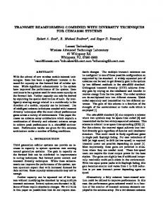
Let ρi = zi , the distance from the ith robot to the receiver. Now suppose the robots are transmitting a common signal, represented by As(t) where A is the amplitude of the transmission signal. For simplicity of analysis, let the message s(t) be the complex sinusoid, i.e., s(t) = e ιωt . Let τi represents the propagation delay from transmitter i to the receiver, and τi = ρi /c. Then the combined received signal, including the noise, by the receiver is r(t) = Fig. 1.

Robots on a grid.

II. P ROBLEM F ORMULATION In this section, we introduce the system model and then present the problem formulation. A. System Model We consider a system of m mobile robots, labeled 1 through m, transmitting a signal representing a common message to a receiver. Each robot is equipped with an isotropic antenna so that a signal is radiated uniformly in all directions. The model of robots on a grid (see Fig. 1) is considered. That is, each robot can move to one of the four adjacent locations (North, South, East, West) at each step only if the adjacent location is not occupied by others or obstacles. We list the assumptions for the system in the following. (a) The robots can detect objects when they have a short distance to them (e.g., less than r¯ where r¯ is the sensing radius of each robot and is assumed to be greater than one-fourth of the wavelength λ). (b) The clocks on the robots are not perfectly synchronized, which may lead to unknown phase offsets for the robots. We denote the offsets by η 1 , . . . , ηm , respectively. (c) Carrier frequency synchronization is achieved in advance. For instance, one approach for frequency synchronization is to employ a master-slave architecture [10], where “slave” nodes use phase-locked loops (PLLs) to lock to a reference carrier signal broadcasted by a “master” node.

m 

μi As(t − τi − ηi ) + n(t),

i=1

where n(t) is white, zero-mean Gaussian noise with power σ 2 , ηi is the phase offset (as a result of clock synchronization errors), and μ i represents the signal attenuation from transmitter i to the receiver which is inversely proportional to the distance ρi , i.e., μi = ρνi for some ν > 0. Then the power of the received signal, not including noise, is  m 1 T /2  νA 2 Pr = | s(t − τi − ηi )| dt T −T /2 i=1 ρi  m ν 2 A2 T /2  1 ιw(t−τi−ηi ) 2 | e | dt = T −T /2 i=1 ρi = ν 2 A2 |

m  1 −ιw(τi+ηi ) 2 e | . ρ i=1 i

Without loss of generality, we let σ 2 = 1. Moreover, we introduce the wave number k = ω/c and the wavelength λ = 2π/k. The signal-to-noise ratio (SNR) is therefore expressed as F (z) =ν 2 A2 |

m  1 −ιw(τi +ηi ) 2 e | ρ i=1 i

m m  1 ιk(ρi +ζi )  1 −ιk(ρj +ζj ) =ν 2 A2 ( e )( e ) ρ ρ i=1 i j=1 i

=

m  ν 2 A2 j=1

ρ2i

+

+

m  ν 2 A2 j=2

m  j=1,j=2

B. Notations Throughout the paper, ι represents the imaginary unit,  ·  indicates the Euclidean 2-norm, c is the speed of light, and the notation [·]+ means that it is zero when the value in the square bracket is less than zero otherwise it has the same value. We refer the robots as the transmitters and the remote station as the receiver.

=

m  m  ν 2 A2 i=1 j=1

ρi ρj

ρ1 ρj

eιk(ρ1 +ζ1 −ρj −ζj )

ν 2 A2 ιk(ρ2 +ζ2 −ρj −ζj ) e + ··· ρ2 ρj

cos k(ρi + ζi − ρj − ζj ),

where ζi = cηi . The formula of F (z) indicates that the SNR depends on the distribution of the m robots and the time difference between them. D. Distributed Transmit Beamforming Problem

C. SNR Formula Consider a coordinate frame with the origin located at the receiver and denote the positions of the m mobile robots at time t by z1 (t), . . . , zm (t). The aggregate position vector is z = (z1 , . . . , zm ) ∈ R2m .

In the paper, we are going to exploit the mobility of the antennas to achieve optimal transmit beamforming. This problem is equivalent to finding a distributed algorithm whereby each robot moves independently while collectively they reach a global optimal configuration that maximizes the SNR at the

receiver 2π/k

2π/k

40 30

20 10

0 −10

−20

Fig. 2. A configuration that maximizes the SNR when the phase offsets ηi ’s are all zero.

receiver. To satisfy practical requirements, we introduce two constraints: (a) The m robots are confined in a given region S on the grid, where the region S is bounded but with irregular obstacles inside. (b) The separation distance L ij =  zi − zj  between any two robots should be always greater than λ/4 in order to minimize the effects of mutual interference [1] and also to avoid collisions. If the m robots are aware of the accurate distances to the receiver and the exact phase offsets, then the solution to the problem is trivial. It can be shown that the maximum of F (z) is achieved when [k(ρ i + ζi ) mod 2π] = [k(ρj + ζj ) mod 2π] for any i and j (see also [8]). Fig. 2 shows an example of one configuration that maximizes the SNR when the phase offsets ηi ’s are all zero (i.e., the clocks are perfectly synchronized). The robots (transmitters) are positioned on concentric circles centered at the receiver with 2π/k distance between them. However, in practice, it is unlikely that robots can measure the distance to the remote receiver. Moreover, the clocks are rarely perfectly synchronized. Thus, in the paper, we assume that each robot can only receive a feedback message of the current SNR from the powerful receiver and can only leverage this feedback information to adjust its position locally. Eventually, the m robots are expected to converge to an optimal configuration in the region S when every robot iteratively updates its position. III. A LGORITHM D ESCRIPTION In this section, we present a distributed algorithm for each robot to update its position using only feedback information from the receiver. The distributed algorithm is probabilitybased, similar to the simulated annealing algorithm [7]. We show that using this protocol, the group of m robots asymptotically converges to an optimal configuration maximizing the SNR with probability one. The proposed distributed algorithm guides each robot toward a global optimal configuration in the region S by performing a sequence of “stop-and-go” maneuvers. A stopand-go maneuver takes place at rounds. Each round is divided to two consecutive intervals: a communication period and a maneuvering period. During a communication period T , the robot transmits at the beginning and receives the SNR feedback in the end. During a maneuvering period, the robot moves from its current position to one of its adjacent spots and

−30

−40 −40

−30

−20

−10

0

10

20

30

40

Fig. 3. An initial randomly deployed configuration of 12 robots in the grid satisfying both constraints. The blue objects of irregular shapes are the obstacles.

again come to rest. We assume that max{η 1 , . . . , ηn }  T , e.g., synchronization errors are much smaller than the communication period such that transmission of m robots will overlap most of the time. So the receiver is able to obtain the SNR when all m robots transmit at the same time. Let Ni (t) be the set of adjacent locations of z i (t) on the grid that are not occupied at time t and meet the two constraints (a) and (b). That is, if x ∈ N i (t), then x is an adjacent location of robot i’s position at t and satisfies x ∈ S and x − zj (t) > λ/4 for any j = i. Let ni (t) denote the cardinality of the set N i (t) at time t. Denote zx−i (t) the new aggregate position vector with the ith component z i (t) replaced by x, i.e., zx−i (t) = (z1 (t), . . . , zi−1 (t), x, zi+1 (t), . . . , zm (t)). Suppose that every robot i can receive the feedback information of the SNR F (z(t)) from the receiver and also the SNR x (t)) when it moves to an adjacent location while the F (z−i others are stationary. At each step, only one robot is allowed to move and it moves to a new location x ∈ N i (t) according to the following probability:  + x − F (z(t)) − F (z−i (t)) 1 exp , (1) qzi (t)→x = ni (t) α(t) 2

m where α(t) = ln(t+1) . α(t) is a positive parameter depending on time t, and it determines how fast the algorithm converges. The probability for robot i to remain in the current location is  1− qzi (t)→x . x∈Ni (t)

This local updating rule means that if a robot moves to an adjacent location for which the receiver has a worse SNR, then the probability of going to that location decreases in terms of an exponential function. The algorithm requires that at each step, only one robot is allowed to update the position. To implement this scheme in practice, we can simply label the robots and let the receiver send a label message in each round to indicate who could move in this round. Next we show that the group of m robots asymptotically converges to an optimal configuration maximizing the SNR

40

40

40

30

30

30

20

20

20

10

10

10

0

0

0

−10

−10

−10

−20

−20

−20

−30

−30

−40 −40

−30

−20

−10

0

20

10

30

40

−40 −40

−30

−30

−20

−10

0

10

20

30

40

−40 −40

−30

−20

−10

0

10

20

30

40

(a) case 1 (b) case 2 (c) case 3 Fig. 4. The final configuration achieved by the 12 robots for 3 cases: (a) The receiver was at [0, 800], and the clocks were not perfectly synchronized; (b) The receiver was at [80, 80], and the clocks were not perfectly synchronized; (c) The receiver was at [80, 80], and the clocks were perfectly synchronized.

when performing the proposed distributed algorithm. Theorem 3.1: Suppose that a group of m robots initially satisfy the two constraints (a) and (b). If α(t) > 0 is nonincreasing and satisfies lim α(t) = 0,

t→∞

α(t) ≥

(2a)

2

m , ln(t + 1)

(2b)

then the m robots converge to an optimal configuration maximizing the SNR with probability one. The proof is given in Appendix. The monotonicity of α(t) decreasing to zero ensures that each robot gets less and less opportunity to enter bad locations, while the condition (2b) guarantees the convergence to a global optimal configuration rather than being trapped in a local optimal one. IV. VALIDATION R ESULTS To verify our distributed algorithm, we studied the configuration of 12 robots in an 80 × 80 square grid (region S) with several obstacles inside. As shown in Fig. 3, the 80 × 80 square grid was located in [−40, 40] × [−40, 40], and each square was at a size of 0.03m × 0.03m. We considered the communication frequency of 433M Hz (the wavelength λ is about 0.69m) and assume νA = 1. The robots were initially placed at random spots in the grid satisfying the constraints (a) and (b). (Notice that if the initial distribution does not satisfy the constraint (b), then a repulsive potential based approach [6] can be adopted to push them away from each other so that the constraint becomes satisfied.) We present simulations in the following three scenarios: 1) The receiver was at [0, 800], and the clocks were not perfectly synchronized; 2) The receiver was at [80, 80], and the clocks were not perfectly synchronized; 3) The receiver was at [80, 80], and the clocks were perfectly synchronized. For the above three cases, the final spatial configurations of the 12 robots are provided in Fig. 4(a), Fig. 4(b), and Fig. 4(c), respectively.

From the simulation results, we observed that the robots approximately converge to the concentric circles centered at the receiver with a separation of at least λ/4 for any pair of robots. The nearby concentric circles have the distance of the wavelength λ between each other providing the best transmitting quality. For case 1 and 2, since the clocks are not perfectly synchronized, the robots in the final configurations in Fig. 4(a) and Fig. 4(b) are a little bit shifted away from the concentric circles. These shifts actually compensate the phase offsets caused by the timing synchronizing errors. For case 3, the robots lie on exactly the concentric circles in the final configuration (Fig. 4(c)) because no phase offset is present due to prefect timing synchronization. V. C ONCLUSIONS We proposed a distributed transmit beamforming algorithm, which utilizes the additional degree of freedom provided by the mobility of antennas to form “beams” towards the receiver. According to the algorithm, the mobile antennas sequentially adjust their positions based on the feedback information of signal-to-noise-ratio (SNR) from the receiver. We have validated and proved that the proposed algorithm are guaranteed to converge to a global optimal configuration. ACKNOWLEDGMENT The work was supported in part, by National Natural Science Foundation of China (60875074), Qianjiang Talents Program (2009R10027), and US National Science Foundation Grant CNS-0845671. A PPENDIX The proof of Theorem 3.1 is similar to the one for the simulated annealing algorithm. We first recall several notions and an important lemma from [4]. Consider a tuple (ϕ, F, N ) where ϕ is a set of a finite number of states, F is a cost function defined on ϕ, and N defines a neighbor relationship for state transition. For any two states x and y in ϕ, the state y is said to be reachable at hight E from x if x = y and F (x) ≥ E, or if there is a sequence of stats x = x0 , x1 , . . . , xk = y for some k ≥ 1 such that xi+1 ∈ N (xi ) and F (xi ) ≥ E for 0 ≤ i ≤ k. If for any real number E and any two states x and y, x is reachable at hight

E from y and y is reachable at hight E from x, then the tuple (ϕ, F, N ) is said to satisfy property WR (weak reversibility). A state x is said to be a local maximum if no state y with F (y) > F (x) is reachable from x at hight F (x). Let x be a local optimal state but not a global optimal one. Then the depth of x is defined to be the smallest number E (E > 0), such that some state y with F (y) > F (x) can be reached from x at height F (x) − E. Finally we say the tuple (ϕ, F, N ) is irreducible if any state in ϕ is reachable from any other state in ϕ. Next, we introduce the lemma. Lemma 5.1: Assume that (ϕ, F, N ) is irreducible and satisfies WR. Suppose the one-step transition probability at step t is pt (x, y)

= P [Xt+1 = y|Xt = x] ⎧ 0 if y ∈ N (x) ∪ {x}, ⎪ ⎪ ⎨ −[F (x)−F (y)]+ 1 if y ∈ N (x), |N (x)| exp αt =

⎪ ⎪ pk (x, z) if y = x, 1− ⎩ z=x

where α1 , α2 , . . . , αt , . . . is a non-increasing sequence of positive numbers and has limit zero. Let d be the maximum of the depths of all states which are local but not global maxima. Let ϕ denote the set of global maxima. Then lim P [Xt ∈ ϕ ] = 1

t→∞

if and only if

∞  t=1

exp (

−d

) = ∞. αt

Proof of Theorem 3.1: Notice that for a bounded set S there are totally a finite number of locations on the grid. We denote the total number of grid nodes in S by n. We construct a graph G = (V, E) with each node representing a configuration of m robots in the region S without overlapping. Thus the n! nodes. Clearly, in our setup (v, v) node set V has (n−m)! is always an edge of the graph (i.e., each node has a loop), meaning that the m robots remain in its current configuration. In addition, a node pair (v, v  ) is an edge of the graph G if the configuration vectors z and z  corresponding to v and v  have only one different component, say z i and zi , where zi and zi are adjacent locations also satisfying the separation constraint. This means that only one robot updates its location from z i to zi while all the others keep stationary. Note that if a robot can move from z i to zi , it can also move from z i to zi . So the graph is undirected. Also, it can be easily observed that the graph is connected. Hence, the transition system is irreducible and satisfies the property WR. According to (1), it follows that the transition probability from one node v to its neighbor node v  has the same formula as defined in Lemma 5.1. Moreover, the sequence α(1), α(2), . . . is non-increasing and has limit zero as stated in Theorem 3.1. Note from the formula of the SNR F (z) that 0 ≤ F (z) ≤ m2 for any z. As a result, the maximum of the depths, d , of all configurations which are local but not global

maxima satisfies

d∗ ≤ m2 .

Then by the condition (2b), we obtain that ∞  t=1

exp (

∞  −d

−d ln(t + 1) )≥ exp ( ) α(t) m2 t=1

≥ =

∞  t=1 ∞  t=1

exp (− ln(t + 1)) 1 = ∞. t+1

Thus, applying Lemma 5.1, it concludes that the m robots eventually converge to an optimal configuration maximizing the SNR with probability one.  R EFERENCES [1] P. J. Bevelacqua and C. A. Balanis, “Optimizing antenna array geometry for interference suppression,” IEEE Transactions on Antennas and Propagation, vol. 55, no. 3, pp. 637–641, 2007. [2] I. Bradaric, G. T. Capraro, and M. C. Wicks, “Waveform diversity for different multistatic radar configurations,” in Proceedings of the 41st Asilomar Conference on Signals, Systems and Computers, Pacific Grove, CA, 2007, pp. 2038–2042. [3] P. Fertl, A. Hottinen, and G. Matz, “Perturbation based distributed beamforming for wireless relay networks,” in Proceedings of IEEE Globecom, New Orleans, USA, 2008. [4] B. Hajek, “Cooling schedules for optimal annealing,” Mathematics of Operations Research, vol. 13, no. 2, pp. 311–329, 1988. [5] S. Haykin, Adaptive Filter Theory. Singapore: Pearson Education, 2003. [6] A. Howard, M. J. Mataric, and G. S. Sukhatme, “Mobile sensor network deployment using potential fields: A distributed, scalable solution to the area coverage problem,” in Proceedings of 2002 International Conference on Distributed Autonomous Robotic Systems, Fukuoka, Japan, 2002, pp. 299–308. [7] S. Kirkpatrick, “Optimization by simulated annealing,” Journal of Statistical Physics, vol. 34, no. 5, pp. 975–986, 1984. [8] L. Koch, “Multi-vehicle systems as mobile antenna arrays,” Master’s thesis, University of Toronto, 2008. [9] C. K. E. Lau, R. S. Adve, and T. K. Sarkar, “Minimum norm mutual coupling compensation with applications in direction of arrival estimation,” IEEE Transactions on Antennas and Propagation, vol. 52, no. 8, pp. 2034–2041, 2004. [10] R. Mudumbai, G. Barriac, and U. Madhow, “On the feasibility of distributed beamforming in wireless networks,” IEEE Transactions on Wireless Communications, vol. 6, no. 5, pp. 1754–1763, 2007. [11] R. Mudumbai, D. Brown, U. Madhow, and H. Poor, “Distributed transmit beamforming: challenges and recent progress,” IEEE Communications Magazine, vol. 47, no. 2, pp. 102–110, 2009. [12] R. Mudumbai, J. Hespanha, U. Madhow, and G. Barriac, “Scalable feedback control for distributed beamforming in sensor networks,” in Proceedings of the 2005 International Symposium on Information Theory, Adelaide, Australia, 2005, pp. 137–141. [13] H. Ochiai, P. Mitran, H. V. Poor, and V. Tarokh, “Collaborative beamforming for distributed wireless ad hoc sensor networks,” IEEE Transactions on Signal Processing, vol. 53, no. 11, pp. 4110–4124, 2005. [14] T. Trump and B. Ottersten, “Estimation of nominal direction of arrival and angular spread using an array of sensors,” Signal Processing, vol. 50, no. 1-2, pp. 57–69, 1996. [15] E. Visotsky and U. Madhow, “Optimum beamforming using transmit antenna arrays,” in Proceedings of 49th Vehicular Technology Conference, Houston, Texas, USA, 1999, pp. 851–856. [16] P. Xia and G. B. Giannakis, “Design and analysis of transmitbeamforming based on limited-rate feedback,” IEEE Transactions on Signal Processing, vol. 54, no. 5, pp. 1853–1863, 2006. [17] K. Zarifi, S. Affes, and A. Ghrayeb, “Distributed beamforming for wireless sensor networks with random node location,” in Proceedings of 2009 IEEE International Conference on Acoustics, Speech and Signal Processing, Taipei, Taiwan, 2009, pp. 2261–2264.