Distributed Transmit Beamforming using Feedback Control - arXiv

1

Distributed Transmit Beamforming using Feedback Control R. Mudumbai, Student Member, IEEE, J. Hespanha, Senior Member, IEEE, U. Madhow, Fellow, IEEE

arXiv:cs/0603072v1 [cs.IT] 18 Mar 2006

and G. Barriac, Member, IEEE

Abstract— A simple feedback control algorithm is presented for distributed beamforming in a wireless network.

tion, wireless networks, sensor networks, space-time communication.

A network of wireless sensors that seek to cooperatively transmit a common message signal to a Base Station (BS)

I. I NTRODUCTION

is considered. In this case, it is well-known that substantial energy efficiencies are possible by using distributed

Energy efficient communication is important for wire-

beamforming. The feedback algorithm is shown to achieve

less ad-hoc and sensor networks. We consider the prob-

the carrier phase coherence required for beamforming

lem of cooperative communication in a sensor network,

in a scalable and distributed manner. In the proposed

where there are multiple transmitters (e.g., sensor nodes)

algorithm, each sensor independently makes a random adjustment to its carrier phase. Assuming that the BS is

seeking to transmit a common message signal to a distant

able to broadcast one bit of feedback each timeslot about

Base Station receiver (BS). In particular, we investigate

the change in received signal to noise ratio (SNR), the

distributed beamforming, where multiple transmitters

sensors are able to keep the favorable phase adjustments

coordinate their transmissions to combine coherently

and discard the unfavorable ones, asymptotically achiev-

at the intended receiver. With beamforming, the sig-

ing perfect phase coherence. A novel analytical model is derived that accurately predicts the convergence rate. The

nals transmitted from each antenna undergo constructive

analytical model is used to optimize the algorithm for

interference at the receiver, the multiple transmitters

fast convergence and to establish the scalability of the

acting as a virtual antenna array. Thus, the received

algorithm.

signal magnitude increases in proportion to number of

Index Terms— Distributed beamforming, synchroniza-

transmitters N , and the SNR increases proportional to N 2 , whereas the total transmit power only increases

This work was supported by the National Science Foundation under

proportional to N . This N -fold increase in energy ef-

grants CCF-0431205, ANI-0220118 and EIA-0080134, by the Office

ficiency, however, requires precise control of the carrier

of Naval Research under grant N00014-03-1-0090, and by the Institute for Collaborative Biotechnologies through grant DAAD19-03-D-0004 from the U.S. Army Research Office. R. Mudumbai, J. Hespanha and U. Madhow are with the Department

phases at each transmitter in order that the transmitted signals arrive in phase at the receiver. In this paper, we propose a feedback control protocol for achieving

of Electrical and Computer Engineering, University of California Santa Barbara G. Barriac is with Qualcomm Inc., San Diego, CA

such phase coherence. The protocol is based on a fully distributed iterative algorithm, in which each transmitter

2

independently adjusts its phase by a small amount in a

antenna system. This is a challenging problem, because

manner depending on a single bit of feedback from the

even small timing errors lead to large phase errors at the

BS. The algorithm is scalable, in that convergence to

carrier frequencies of interest. Once phase synchroniza-

phase coherence occurs in a time that is linear in the

tion is achieved, reciprocity was proposed as a means

number of cooperating transmitters.

of measuring the channel phase response to the BS. In

Prior work on cooperative communication mainly fo-

this paper, we present an alternative method of achieving

cuses on exploiting spatial diversity for several wireless

coherent transmission iteratively using a simple feedback

relaying and networking problems [1], [2]. Such dis-

control algorithm, which removes the need for explicit

tributed diversity methods require different transmitters

estimation of the channel to the BS, and greatly reduces

to transmit information on orthogonal channels, which

the level of coordination required among the sensors.

are then combined at the receiver. The resulting diver-

Other related work on synchronization in sensor net-

sity gains could be substantial in terms of smoothing

works is based on pulse-coupled oscillator networks

out statistical fluctuations in received power due to

[8] and biologically inspired (firefly synchronization)

fading and shadowing environments. However, unlike

[9] methods. These methods are elegant, robust and

distributed beamforming, distributed diversity does not

suitable for distributed implementation, however they are

provide a gain in energy efficiency in terms of average

limited by assumptions of zero propagation delay and the

received power, which simply scales with the transmitted

requirement of mesh-connectivity, and are not suitable

power. On the other hand, the coherent combining of

for carrier phase synchronization.

signals at the receiver due to distributed beamforming also provides diversity gains.

We consider the following model to illustrate our ideas. The protocol is initialized by each sensor trans-

Recent papers discussing potential gains from dis-

mitting a common message signal modulated by a car-

tributed beamforming include [3], which investigates the

rier with an arbitary phase offset. (This phase offset

use of beamforming for relay under ideal coherence

is a result of unknown timing synchronization errors,

at the receiver, and [4], which shows that even partial

and is therefore unknown.) When the sensors’ wireless

phase synchronization leads to significant increase in

channel is linear and time-invariant, the received signal

power efficiency in wireless ad hoc networks. The beam

is the message signal modulated by an effective carrier

patterns resulting from distributed beamforming using

signal that is the phasor sum of the channel-attenuated

randomly placed nodes are investigated in [5]. However,

carrier signals of the individual sensors. At periodic

the technical feasibility of distributed beamforming is

intervals, the BS broadcasts a single bit of feedback

not investigated in the preceding papers. In our prior

to the sensors indicating whether or not the received

work [6], [7], we recognized that the key technical

SNR level increased in the preceding interval. Each

bottleneck in distributed beamforming is carrier phase

sensor introduces an independent random perturbation

synchronization across cooperating nodes. We presented

of their transmitted phase offset. When this results in

a protocol in which the nodes first establish a common

increased total SNR compared to the previous time

carrier phase reference using a master-slave architecture,

intervals (as indicated by feedback from the BS), the

thus providing a direct emulation of a centralized multi-

new phase offset is set equal to the perturbed phase by

3

each sensor; otherwise, the new phase offset is set equal

channel. This means that each sensor has a flat-

to the phase prior to the perturbation. Each sensor then

fading channel to the receiver. Therefore the sensor

introduces a new random perturbation, and the process

i’s channel can be represented by a complex scalar

continues. We show that this procedure asymptotically

gain hi .

converges to perfect coherence of the received signals,

2) Each sensor has a local oscillator synchronized to

and provide a novel analysis that accurately predicts

the carrier frequency fc i.e. carrier drift is small.

the rate of convergence. We verify the analytical model

One way to ensure this is to use Phase-Locked

using Monte-Carlo simulations, and use it to optimize

Loops (PLLs) to synchronize to a reference tone

the convergence rate of the algorithm.

transmitted by a designated master sensor as in

The rest of this paper is organized as follows. Sec-

[6]. In this paper, we use complex-baseband nota-

tion II describes our communication model for the

tion for all the transmitted signals referred to the

sensor network. A feedback control protocol for dis-

common carrier frequency fc .

tributed beamforming is described in Section III-A and

3) The local carrier of each sensor i has an unknown

its asymptotic convergence is shown in Section III-B.

phase offset, γi relative to the receiver’s phase

Section IV describes an analytical model to characterize

reference. Note that synchronization using PLLs

the convergence behavior of the protocol. Some ana-

still results in independent random phase offsets

lytical and simulation results are presented in Section

γi = (2πfc τi

V. Section V-A presents an optimized version of the

synchronization errors τi that are fundamentally

feedback control protocol. Sections V-B and V-C present

limited by propagation delay effects.

mod

2π), because of timing

some results on scalability, and the effect of time-varying

4) The sensors’ communication channel is time-

channels respectively. Section VI concludes the paper

slotted with slot length T . The sensors only trans-

with a short discussion of open issues.

mit at the beginning of a slot. This requires some

II. C OMMUNICATION M ODEL FOR A S ENSOR N ETWORK We consider a system of N sensors transmitting a

coarse timing synchronization: τi ≪ T where τi is the timing error of sensor i. 5) Timing errors among sensors are small compared to a symbol interval (a “symbol interval” Ts is 1 B ).

common message signal m(t) to a receiver. Each sensor

nominally defined as inverse bandwidth: Ts =

is power constrained to a maximum transmit power of

For a digitally modulated message signal m(t),

P . The message m(t) could represent raw measurement

this means that Inter Symbol Interference (ISI) can

data, or it could be a waveform encoded with digital

be neglected.

data. We now list the assumptions in this model.

6) The channels hi are assumed to exhibit slow-

1) The sensors communicate with the receiver over

fading, i.e. the channel gains stay roughly constant

a narrowband wireless channel at some carrier

for several time-slots. In other words Ts ≪ T ≪

frequency, fc . In particular, the message bandwidth

Tc , where Tc is the coherence time of the sensor

B < Wc , where B is the bandwidth of m(t) and

channels.

Wc is the coherence bandwidth of each sensor’s

4

tion process begins with the receiver broadcasting a

equality, we can see that to maximize G, it is necessary . that the received carrier phases Φi = γi + θi + ψi , are

signal to the sensors to transmit their measured data.

all equal:

The sensors then transmit the message signal at the next

N X ai bi ejΦi G=

Distributed transmission model: The communica-

time-slot. Specifically, each sensor transmits: si (t) = A· gi m(t − τi ), where τi is the timing error of sensor √ i, A ∝ P is the amplitude of the transmission, and gi is a complex amplification performed by sensor i. Our objective is to choose gi to achieve optimum received SNR, given transmit power constraint of P on each sensor. For simplicity, we write hi = ai ejψi and gi = bi e

jθi

, where bi ≤ 1 to satisfy the power constraint. Then

the received signal is: r(t) =

N X

i=1

N X ai ejΦi ≤ i=1

N X √
√ jΦi
= ai ai e

(5)

i=1

≤ Gopt ≡

N X i=1


ai , with equality if and only if Φi = Φj and bi = 1 (6)

However sensor i is unable to estimate either γi or ψi because of the lack of a common carrier phase reference.

hi si (t)e

jγi

+ n(t)

(1)

In the rest of this paper, we propose and analyze a

i=1

=A

hi gi ejγi m(t − τi ) + n(t)

N X

ai bi ej(γi +θi +ψi ) m(t − τi ) + n(t).

i=1

=A

feedback control technique for sensor i to dynamically

N X

i=1

compute the optimal value of θi so as to achieve the condition for equality in (6). (2) III. F EEDBACK C ONTROL P ROTOCOL

In the frequency domain, this becomes: R(f ) = A

N X

ai bi ej(γi +θi +ψi ) M (f )e−jf τi + N (f )

i=1

≈ A· M (f )

N X

ai bi ej(γi +θi +ψi ) + N (f ),

(3)

i=1

where n(t) is the additive noise at the receiver and N (f ) is its Fourier transform over the frequency range f ≤

Fig. 1.

Phase synchronization using receiver feedback

B 2.

In (1), the phase term γi accounts for the phase offset

Fig. 1 illustrates the process of phase synchronization

in sensor i. In (3), we set e−jf τi ≈ 1 because f τi ≤

using feedback control. In this section, we describe the

≪ 1. Equation (3) motivates a figure of merit

feedback control algorithm, and prove its asymptotic

Bτi ≡

τi Ts

for the beamforming gain: N X ai bi ej(γi +θi +ψi ) G=

convergence. (4)

i=1

A. Description of Algorithm

which is proportional to the square-root of received SNR.

The protocol for distributed beamforming works as

Note that bi ≤ 1, in order to satisfy the power

follows: each sensor starts with an arbitrary (unsyn-

constraint on sensor i. From the Cauchy-Schwartz In-

chronized) phase offset γi . In each time-slot, the sensor

5

applies a random perturbation to θi and observes the

The algorithm works as follows.

resulting received signal strength y[n] through feedback.

Initially the phases are set to zero: θi [1] = 0. At each

The objective is to adjust its phase to maximize y[n]

time-slot n, each sensor i applies a random phase pertur-

through coherent combining at the receiver. Each phase

bation δi [n] to θi [n] for its transmission. As a result, the

perturbation is a guess by each sensor about the cor-

received phase is given by: Φi [n] = γi +θi [n]+δi [n]+ψi .

rect phase adjustment required to increase the overall

The BS measures Y[n] and keeps a record of the highest

received signal strength. If the received SNR is found to

observed signal strength Ybest [n] = maxk Ybest [n] θi [n + 1] =  θi [n] otherwise.

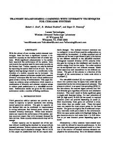
N = 10 sensors. 0 iterations 90 120 60

10 iterations 90 120 60

150

30

180

0 330

210 240

270

150 180

300

240

30

180

0

240

330 270

330 270

300

300

(8)

This has the effect of retaining the phase perturbations 30

150 180

0

210 240

signal strength:   Ybest [n + 1] = max Ybest [n], Y[n]

500 iterations 90 60 120

150

Simultaneously, The BS also updates its highest received

0

210

50 iterations 90 60 120

210

30

(7)

330 270

300

that increase SNR and discarding the unfavorable ones that do not increase SNR. The sensors and the BS repeat the same procedure in the next timeslot. The random perturbation δi [n] is chosen indepen-

Fig. 2.

Convergence of feedback control algorithm

dently across sensors from a probability distribution δi [n] ∼ fδ (δi ), where the density function fδ (δi ) is a

Let n denote the time-slot index and Y[n] the ampli-

parameter of the protocol. In this paper, we consider

tude of the received signal in time-slot n. From (3), we P have: Y[n] ∝ i ai ejΦi [n] where Φi [n] is the received

primarily two simple distributions for fδ (δi ): (i) the two valued distribution where δi = ±δ0 with proba-

signal phase corresponding to sensor i. We set the pro-

bility 0.5, and (ii) the uniform distribution where δi ∼

portionality constant to unity for simplicity of analysis.

uniform[−δ0 , δ0 ]. We allow for the possibility that the

At each time instant n, let θi [n] be the best known

distribution fδ (δi ) dynamically changes in time.

carrier phase at sensor i for maximum received SNR.

It follows from (7) that if the algorithm were to

Each sensor uses the distributed feedback algorithm to

be terminated at timeslot n, the best achievable signal

dynamically adjust θi [n] to satisfy (6) asymptotically.

strength using the feedback information received so

6

far, is equal to Ybest [n], which correspond to sensor i transmitting with the phase θi [n].

¯ We now provide an argument the starting phase angles φ. that shows (under mild conditions on the probability den-

X Φ [n] ai e i Ybest [n] ≡

sity function fδ (δi )), that in fact {Ybest [n]} converges to

i

where Φi [n] = γi + θi [n] + ψi

Bound [10]. In general the limit G0 would depend on

(9)

the constant Gopt with probability 1 for arbitrary starting ¯ The following proposition will be needed to phases φ. establish the convergence.

B. Asymptotic Coherence We now show that the feedback control protocol

Proposition 1: Consider a distribution fδ (δi ) that has

outlined in Section III-A asymptotically achieves phase

non-zero support in an interval (−δ0 , δ0 ). Given any

¯ coherence for any initial values of the phases Φi . Let Φ

¯ < Gopt − ǫ, where ǫ > 0 is φ¯ 6= ¯0, and Mag(φ)

denote the vector of the received phase angles Φi . We

arbitrary, there exist constants ǫ1 > 0 and ρ > 0 such

¯ to be the received signal define the function Mag(Φ)

¯ − Mag(φ) ¯ > ǫ1 ) > ρ. that P rob(Mag(φ¯ + δ) Proof. For the class of distributions fδ (δi ) that we

¯ strength corresponding to received phase Φ: . X jΦi ¯ = ai e Mag(Φ)

consider, the probability of choosing δi in any finite (10)

i

Phase coherence means Φi = Φj = Φconst , where Φconst is an arbitrary phase constant. In order to remove this ambiguity, it is convenient to work with the rotated phase values φi = Φi − Φ0 , where Φ0 is a constant

interval I ⊂ (−δ0 , δ0 ) is non-zero. One example of such a class of distributions is fδ (δi ) ∼ uniform[−δ0 , δ0 ]. Recall that the phase reference is chosen such that the P total received signal i ai ejφi has zero phase. First we

sort all the phases φi in the vector φ¯ in the descending

chosen such that the phase of the total received signal

order of |φi | to get the sorted phases φ∗i satisfying |φ∗1 | >

is zero. This is just a convenient shift of the receiver’s

|φ∗2 | > ... > |φ∗N |, and the corresponding sorted channel

phase reference and as (10) shows, such a shift has no

¯ < Gopt − ǫ to gains a∗i . We use the condition Mag(φ)

impact on the received signal strength:

get:

¯ ≡ Mag(Φ) ¯ Mag(φ)

(11)

We interpret the feedback control algorithm as a discrete-time random process Ybest [n] in the state-space

cos(φ∗1 )

X i

a∗i
φǫ = cos−1 P ∗ i ai

(12)

¯ the state-space being the N -dimensional space of φ,

Now we choose a phase perturbation δ1 that decreases

of the phases φi constrained by the condition that the

|φ∗1 |. This makes the most mis-aligned phase in φ¯ closer

phase of the received signal is zero. We observe that the

to the received signal phase, and thus increases the

sequence {Ybest [n]} is monotonically non-decreasing,

magnitude of the received signal. If φ∗1 > 0, then we

and is upperbounded by Gopt as shown in (5). Therefore

need to choose a δ1 < 0, whereas if φ∗1 < 0, we need

each realization of {Ybest [n]} is always guaranteed to

δ1 > 0. In the following, we assume that φ∗1 > 0 and

converge to some limit G0 ≤ Gopt . Furthermore G0 =

φǫ > δ0 . The argument below does not depend on these

limn→∞ Ybest [n] ≡ supn→∞ Ybest [n] i.e. the limit G0

assumptions, and can be easily modified for the other

of the sequence {Ybest [n]} is the same as its Least Upper

cases. Consider δ1 ∈ (−δ0 , − δ20 ). This is an interval in

7

which fδ (δ1 ) is non-zero , therefore there is a non-zero

¯ considered in Proposition 1, starting from an arbitrary φ,

probability ρ1 > 0 of choosing such a δ1 . We have:

the feedback algorithm converges to perfect coherence of

a∗1 cos(φ∗1 + δ1 ) − a∗1 cos(φ∗1 ) > 2ǫ1 ∗ ∗ . a sin(φǫ − where ǫ1 = 1 4

δ0 2 )δ0

the received signals almost surely, i.e. Ybest [n] → Gopt (13)

The perturbation δ1 by itself will achieve a non-zero increase in total received signal, provided that the other phases φ∗i do not get too mis-aligned by their respective δi : ¯ − Mag(φ) ¯ = Mag(φ¯ + δ)

i

¯ or equivalently φ[n] → ¯0 (i.e. φi [n] → 0, ∀i) with

probability 1.

¯ We observe that ǫ1 and ρ1 do not dependent on φ.

X

Theorem 1: For the class of distributions fδ (δi )


a∗i cos(φ∗i + δi ) − cos(φ∗i )

Proof: We wish to show that the sequence Ybest [n] =

¯ ¯ ¯ Mag(φ[n]) → Gopt given an arbitrary φ[1] = φ.

¯ Consider an arbitrarily small ǫ > 0 and define Tǫ (φ) as the first timeslot when the received signal exceeds Gopt − ǫ.

¯ then Ybest [n] = By definition if n < Tǫ (φ),

¯ Mag(φ[n]) < Gopt − ǫ,
and by Proposition 1,
X a∗i cos(φ∗i + δi ) − cos(φ∗i ) = a∗1 cos(φ∗1 + δ1 ) − cos(φ∗1 ) + P rob(Ybest [n + 1] − Ybest [n] > ǫ1 ) > ρ for some i>1 X
∗ constants ǫ1 > 0 and ρ > 0. We have: a∗i cos(φ∗i + δi ) − cos(φ > 2ǫ1 + i) i>1   ¯ (17) E Ybest [n + 1] − Ybest [n] > ǫ1 ρ, ∀n < Tǫ (φ) (14) ¯ is continuous in each of We note that since Mag(φ) the phases φ∗i , we can always find a ǫi > 0 to satisfy:
ǫ1 ∗ , ∀|δi | < ǫi (15) ai cos(φ∗i +δi )−cos(φ∗i ) < N −1 . ǫ1 In particular the choice ǫi = a∗ (N −1) , satisfies (15), and

Using (17) we have: Gopt ≥ Ybest [n + 1]

n   X = Ybest [1] + Ybest [k + 1] − Ybest [k] k=1

i

¯ With the δi ’s chosen this choice of ǫi is independent of φ.

>

n  X

k=1

to satisfy (15), we have:

 Ybest [k + 1] − Ybest [k]

(18)

Taking expectation we have: −ǫ1
1

a∗i

cos(φ∗i

+ δi ) −

cos(φ∗i )




< ǫ1

(16)

Since fδ (δi ) has non-zero support in each of the nonzero intervals (−ǫi , ǫi ), the probability ρi of choosing δi to satisfy (15) is non-zero, i.e. ρi > 0, which is ¯ Finally, we recall that each of the δi independent of φ. are chosen independently, and therefore with probability Q ρ = i ρi > 0, it is possible to find δ1 to satisfy (13)

Gopt > E

n X

k=1


 Ybest [k + 1] − Ybest [k]

n   X 
¯ >n E ¯ >n > P rob Tǫ (φ) Ybest [k + 1] − Ybest [k] Tǫ (φ) k=1





¯ > n nǫ1 ρ > P rob Tǫ (φ)

(19)

where we obtained (19) by using (17). Therefore we ¯ > n) < have P rob(Tǫ (φ)

1 Gopt n ǫ1 ρ

→ 0, as n → ∞.

and δi , i > 1 to satisfy (15). For δ¯ chosen as above,

Since this is true for an arbitrarily small ǫ, we have

¯ − Mag(φ) ¯ > ǫ1 , and therefore Proposition Mag(φ¯ + δ)

¯ shown that Ybest [n] → Gopt and φ[n] → ¯0 almost

1 follows.



surely.



8

IV. A NALYTICAL M ODEL FOR C ONVERGENCE

The initial value y[1] in (20) is set under the assumption

The analysis in Section III-B shows that the feedback

¯ are randomly distributed in that the received phases φ[1]

control algorithm of Section III-A asymptotically con-

[0, 2π). For subsequent timeslots, Ybest [n + 1] in (21)

verges for a large class of distributions fδ (δi ); however

¯ is conditioned on Ybest [n] but the phase vector φ[n] is

it provides no insight into the rates of convergence.

not known. Some remarks are in order regarding this

We now derive an analytical model based on simple,

definition, particularly the relationship of y[n] with the

intuitive ideas that predicts the convergence behavior

(unconditionally) averaged Ybest [n]. Let

of the protocol accurately. We then use this analytical



. y[n+1] = F y[n] , where F (y) = E Ybest [n+1] Ybest [n] = y

model, to optimize fδ (δi ) for fast convergence.

Consider:

70

received signal strength: y[n]

(22)



 E Ybest [n + 1] = EYbest [n] E Ybest [n + 1] Ybest [n] 
 = EYbest [n] F Ybest [n] 
 ≈ F E Ybest [n] ≡ y[n + 1] (23)

60 50 40 30 20

In most cases, the function F (y) is concave, and there10

fore (by Jensen’s Inequality) the approximation in (23) 0 0

50

100

150

200

250

300

timeslots, n

represents an overestimate of the unconditional average of Ybest [n + 1]. Also in different instances of the

Fig. 3.

Motivating the Analytical Model: two simulated instances

with N = 100, fδ (δi ) ∼

π π uniform[− 20 , 20 ].

algorithm, we would expect to see different random ¯ evolutions of φ[n] and Ybest [n] with time, and an averaged quantity only provides partial information about the convergence rate. Fortunately, as Fig. 3 shows, even

A. Derivation of Analytical Model

over multiple instances of the algorithm, the convergence

The basic idea behind our analytical model is that

rate remains highly predictable, and the average charac-

the convergence rate of typical realizations of Ybest [n]

terizes the actual convergence reasonably well. Since the

is well-modeled by computing the expected increase in

variation of the random Ybest [n] around its average value

signal strength at each time-interval given a distribution

is small, the approximation in (23) also works well. Our

fδ (δi ). This is illustrated in Fig. 3, where we show

goal is to compute F (y) as defined in (22).

two separate realizations of Ybest [n] from a Monte-Carlo simulation of the feedback algorithm.

Note that while (22) is conditioned on Ybest [n] being

¯ known, the phase vector φ[n] is unknown. As Ybest [n]

We define the averaged sequence y[n] recursively as

increases, the phases φi [n] become increasingly clustered

the conditional value of Ybest [n + 1] given Ybest [n]:   ¯ y[1] = E Mag(φ[1]) (20)   y[n + 1] = Eδ[n] Ybest [n + 1] Ybest [n] = y[n] (21) ¯

together, however their exact values are determined by their initial values, and the random perturbations from previous time-slots. In order to compute the expectation ¯ in (22), we need some information about φ[n].

9

We show in Section IV-B that the phases φi [n] can be accurately modeled as clustered together according to a statistical distribution that is determined parametrically as a function of Ybest [n] alone. This is analogous to the technique in equilibrium statistical mechanics, where the individual positions and velocities of particles in an ensemble is unknown, but accurate macroscopic results are obtained by modeling the kinetic energies as following the Boltzmann distribution, which is fully determined

(CLT). X ¯ = ai ejφi +jδi Mag(φ¯ + δ)

X X
ai cos φi sin δi ai cos φi cos δi − sin φi sin δi + j = i

i


= Cδ y[n] + x1 + jx2 ,

(28)


(29) where Cδ = Eδ cos δi ,   X
ai cos φi cos δi − Cδ − sin φi sin δi , x1 = i

(30)

by a single parameter (the average kinetic energy or the temperature). In our case, φi [n] are modeled as indepen-

(27)

i

 X  ai cos φi sin δi + sin φi cos δi x2 = i

dent and identically distributed (for all i) according to a

(31)

distribution satisfying the constraint: The random variables x1 , x2 are illustrated in Fig. 4. y[n] =

X i



ai cos φi ≡ N E ai Eφi cos φi

(24)

Therefore, even though the individual φi are unknown, we can compute all aggregate functions of φ¯ using this distribution, as if the φi are known. This is an extremely powerful tool, and we now use it to compute F (y)

Fig. 4.

Perturbation in the total received signal.

¯ treating φ[n] as a given. Section IV-B completes the computation by deriving the distribution used to specify ¯ given Ybest [n]. φ[n]

binations of iid random variables, sin δi and cos δi . Therefore as the number of sensors N increases, these

From the condition Ybest [n] = y[n], we have: y[n] =

X

ai ejφi =

i

X

ai cos φi

random variables can be well-modeled as Gaussian, as (25)

i

received signal is zero for our choice of phase reference. We have the following expressions (omitting the time¯ and δ[n] ¯ for convenience): index on φ[n]   ¯ Mag(φ¯ + δ)  y[n]

per the CLT [11]. Futhermore, x1 , x2 are zero-mean random variables, and their respective variances σ12 , σ22

where we used the fact that the imaginary part of the

Ybest [n + 1] =

Both x1 and x2 as defined in (28) are linear com-

¯ > y[n] if Mag(φ¯ + δ) otherwise.

are related by:  1 X 2 ai (1 − Cδ2 ) − cos(2φi )(Cδ2 − C2δ ) 2 i  1 X 2 ai 1 − cos(2φi )C2δ σ22 = 2 i
(32) where C2δ = Eδ cos(2δi ) σ12 =

(26)

With these simplifications, the statistics of y[n + 1]

¯ as a sum of i.i.d. terms We now express Mag(φ¯ + δ)

only depends on the density function fδ (δi ) through Cδ

from each sensor, and invoke the Central Limit Theorem

and C2δ . We have the following proposition.

10

Proposition 2: Assuming that the CLT applies for

phases φi are distributed independently1 and uniformly

random variable x1 , the expected value of the received

in [0, 2π). In particular, we set ai = 1 for all sensors,

signal strength is given by: 2   δ )) σ1 − (y[n](1−C 2 2σ1 y[n + 1] ≈ y[n] 1 − p· (1 − Cδ ) + √ e 2π (33)  y[n](1 − C )  δ (34) where p = Q σ1

which gives Gopt = N . As the algorithm progresses

Proof. First we observe that the small imaginary component x2 of the perturbation mostly rotates the received signal, with most of the increase in y[n + 1]

towards convergence, the values of φi are distributed over a smaller and smaller range. In general, we expect that the distribution fφ (φi ) of φi [n] depends on the number of sensors N , the iteration index n, and the distribution of the perturbations fδ (δi ). In the spirit of the statistical model, we consider large N , and look for a class of distributions that approximate fφ (φi ).

coming from x1 (see Fig. 4).

0.25

≈ Cδ y[n] + x1




(35)

Defining p as the probability that Ybest [n + 1] > y[n], (33), (34) readily follow from (35), (26) using Gaussian statistics.



We can rewrite (33) as:

y[n + 1] = F y[n] = y[n] + f y[n]  y(1 − C )  . δ where f (y) = σ1 g σ1 x2 . 1 and g(x) = √ e− 2 − xQ(x) 2π

Probability Density

¯ = Cδ y[n] + x1 + jx2 Mag(φ¯ + δ)

0.2

0.15

0.1

0.05

0 −2

−1.5

−1

−0.5

0

0.5

1

1.5

Phase angle (radians) (36)

Proposition 2 does not yet allow us to compute the

Fig. 5.

Comparing a Laplacian Distribution with a Histogram of

Empirically Observed Phase Angles

y[n] because it involves the variance σ1 that depends on the phases φi of the individual sensors. In the next section we present a statistical distribution for φi that allows us to calculate aggregate quantities such as σ1 without knowledge of the individual φi . B. Statistical Characterization of Sensor Channels The statistical model is based on the assumption that each sensor has a channel to the BS of similar quality,

We find that the Laplacian probability distribution gives the best results2 in terms of accurately predicting the convergence behavior of the algorithm of Section III-A. Fig. 5 shows an empirically derived histogram 1 It

is important to note that the φi are not random variables, however

we statistically parametrize them using a probability distribution for the sake of compactness. 2 The

Laplacian distribution for φi is empirically found to work well,

and unknown phase. This means that the ai ’s are all

when compared with other families of distributions like the uniform

approximately equal, and that the initial values of the

and triangular distributions.

2

11

from a Monte-Carlo simulation of the feedback control

C. Summary of Analytical Model

algorithm. A Laplacian approximation is also plotted

We now summarize the analytical model derived in

alongside the histogram. We now explain the details of

Sections IV-A and IV-B. Our objective is to model

the approximation.

the increase over time of the received signal strength

The Laplacian density function is given by [11]: fφ (φi ) =

i| 1 −|φ e φ0 2φ0

by averaging over all possible values of the random (37)

perturbations. As mentioned before, we set the channel attenuations for each sensor to unity i.e. ai = 1.

For φi distributed according to (37), we also have: 1 1 + φ20
1 E cos 2φi = 1 + 4φ20
E cos φi =

(38)

1) Initially we set the received signal strength as √ y[1] = N . This is the expected value of the signal strength if the initial phase angles are all

(39)

Therefore given that at iteration n of the feedback ¯ = [φ1 φ2 ...φN ], we algorithm, the phase angles are φ[n]

chosen independently in [0, 2π). 2) At each time-interval (iteration) n > 1, given the probability distribution of the perturbations fδ (δi ) and the value of y[n], we compute the Laplacian

have:

parameter φ0 using (41), and then compute the ¯ y[n] = Mag(φ[n]) =

X

ai e

jφi

i

≡

X

cos φi

(40)

i

where we used ai = 1 in (10). Now if we parametrize all the φi using a Laplacian distribution, we can set φ0
P such that i cos φi ≡ N Eφ cos φ . Thus we use (38) to rewrite (40) as:

1] using the Gaussian statistics in (35) and (26). V. P ERFORMANCE A NALYSIS

OF

F EEDBACK

C ONTROL P ROTOCOL We now present some results obtained from the ana-

N y[n] = 1 + φ20

(41)

from a Monte-Carlo simulation with N = 100, for two

Proposition 3: The variance σ12 of x1 is given by: y[n]  N 2 N σ12 = (1 − Cδ2 ) − (C − C ) 2δ δ 2 4 − 3 y[n] N

lytical model of Section IV. Fig. 6 shows the evolution of y[n] derived from the analytical model and also

We are now able to determine σ1 given y[n].

different choices of the distribution fδ (δi ): a uniform

(42)

π π , 30 ] and a distribution choosing distribution in [− 30 π with equal probability. The close match observed ± 30

Proof. Equation (42) follows using (32), and the value of the Laplacian parameter from (41) along with
P the observation that i cos(2φi ) = N Eφ cos(2φ) = N . 1+4φ20

Gaussian variance σ12 using (42) and finally y[n +



between the analytical model and the simulation data provides validation for the analytical model. We observe from Fig. 6, that the received signal grows rapidly in the beginning, but after y[n] gets to within about 25% of Gopt , the rate of convergence becomes

Using Propositions 2 and 3, we are able to analytically

slower. Also while the simple two-valued probability

derive the average convergence behavior of the feedback

distribution appears to give good results, it does not

control algorithm. In particular, we recursively calculate

satisfy the condition for asymptotic coherence derived

y[n] by substituting the variance σ12 from (42) into (33).

in Section III-B.

12

100

received signal strength, y[n]

received signal strength, y[n]

100 90 80 70 60 simulated analytical

50 40 30 20 10 0 0

500

1000

1500

Fig. 6.

80 70

π ) 30

simulated analytical

60 50 40 30 20 10 0 0

2000

timeslot index, n

π , (a) fδ (δi ) ∼ uniform(− 30

90

500

1000

timeslot index, n

1500

2000

π (b) fδ (δi ) ∼ ± 30

Comparison of Analytical Model with Monte-Carlo Simulation of Feedback Control Algorithm

We are interested in δi corresponding to small random

A. Optimizing the Random Perturbations In Fig. 6, we used the same distribution for the perturbations for all iterations of the algorithm. However this choice is not optimal: intuition suggests that it is best to choose larger perturbations initially to speed up the convergence and make the distribution narrower when the phase angles are closer to coherence. We now use the

perturbations i.e. δi ≪

π 2.

For such small values of δi ,

(43) allows only a small range of possible values of C2δ . Indeed we observe that cos(δi ) and cos(2δi ) are very well approximated by the first two terms of the Taylor series: cos(δ) ≈ 1 −

δ2 π , if |δ| ≪ 2 2

(44)

analytical model to dynamically choose the distribution

Equation (44) indicates that both Cδ and C2δ are essen-

fδ (δi ) as a function of y[n]. The general problem of

tially determined by the second moment of δi , and there-

choosing a distribution is a problem in calculus of vari-

fore even a one-parameter family of distributions fδ (δi )

ations. Fortunately, it is possible to restrict ourselves to a

is sufficient to achieve optimality of the convergence

family of distributions without losing optimality, because

rate. Fig. 7 shows plots of the optimal choices of the

the analytical model only depends on the distribution

(Cδ , C2δ ) pair with N = 2000 over 10000 timeslots for

through the two parameters Cδ , C2δ . Furthermore the

two families of distributions: (i) the 3-point distributions

parameters Cδ , C2δ are highly correlated. To see this

P (±δ0 ) = p, P (0) = 1 − 2p parameterised by the

recall from (31) and (32) the definitions of Cδ and C2δ as

pair (δ0 , p), and (ii) the distributions uniform[−δ0 , δ0 ]

the expected values of cos(δi ) and cos(2δi ) respectively.

parametrised by δ0 . At each iteration of the protocol,

Using the identity cos(2δ) = 2 cos2 (δ) − 1 and Jensen’s

we used the analytical model to compute the value of

Inequality, we can show that C2δ is constrained by the

the parameters (i.e. the pair (δ0 , p) in case (i) and δ0

value of Cδ :

in case (ii)) that maximizes the y[n + 1] given y[n]; the optimal parameters in each case were determined 2Cδ2 − 1 ≤ C2δ ≤ 2Cδ − 1

(43)

numerically using a simple search procedure. The two

curves in Fig. 7 were obtained by plotting (Cδ , C2δ ) pair corresponding to the optimal parameters for cases (i) and (ii) at each timeslot. The 3-point distribution is flexible enough to permit any (Cδ , C2δ ) in the feasible region

received signal y[n]

13

200 1.5°

3°

50 0 0

500

1000

1500

2000

2500

3000

500

1000

1500

2000

2500

3000

50 40 30

0

optimum δ in degrees

close to optimal, thereby confirming the intuition of (44).

°

6 100

of (43). For the example of Fig. 7, it is clear that the uniform distribution achieves values of (Cδ , C2δ ) that is

°

10

optimized 150

1 optimized over uniform distributions

0.8

20 10 0 0

timeslots, n

0.6 optimized over general distributions 0.4

C

2δ

0.2

Fig. 8.

0

Optimized algorithm compared to fixed fδ (δi )

∼

uniform[−δ0 , δ0 ] for different δ0 and N = 200

−0.2 Feasible Region

−0.4

B. Scalability Results

−0.6 −0.8 −1 0

We now turn to the analytical model to study the 0.2

0.4

C

0.6

0.8

δ

scalability of the feedback algorithm with the number 1 of transmitting sensors N . We show the following scalability results:

Fig. 7.

Near-Optimality of a One-Parameter Distribution

- The expected received signal strength at any time, always increases when more transmitters are added.

We now use the family of distributions fδ (δi ) ∼

- The number of timeslots required for the expected

uniform[−δ0 , δ0 ] to obtain insight into the optimal con-

signal strength to reach within a certain fraction

vergence rate. Fig. 8 shows y[n] as a function of n for

of convergence always increases with more trans-

fixed values of δ0 as well as for the optimized algo-

mitters, but increases no faster than linearly in the

rithm. We observe that the convergence rate decreases

number of transmitters.

with time in all cases, and the optimized algorithm

Theorem 2: Let y1 [n] and y2 [n] be the expected

converges significantly faster than any fixed instance.

received signal magnitude at timeslot n when the number

Fig. 8 also shows the variation of optimal δ0 with time.

of transmitting sensors is N1 and N2 respectively. If the

This confirms our intuition that at the initial stages of

sensors use the same distributions fδ (δi ) for all timeslots

the algorithm, it is preferable to use larger perturbations

n, and N2 > N1 , then the following holds for all n:

(corresponding to large δ0 ), and when y[n] gets closer to Gopt , it is optimum to use narrower distributions (corresponding to smaller δ0 ).

and

y2 [n] ≥ y1 [n]

(45)

y2 [n] y1 [n] ≥ N1 N2

(46)

14

Proof. We offer a proof by induction. From Section IV-C, we know that y2 [1] > y1 [1] and

y1 [1] N1

y2 [1] N2 .

distributions. We apply Theorem 2 to the case where

To

we use the distribution fδ (δi ) optimized for N1

prove (45), we need to show that y2 [n + 1] > y1 [n + 1]

sensors in both cases. By definition y˜2 [n] ≥ y2 [n], and

given y2 [n] > y1 [n].

y˜1 [n] = y1 [n], therefore y˜2 [n] ≥ y˜1 [n], ∀n. This proves

>

We write y1 [n+1] = F1 (y1 [n]), y2 [n+1] = F2 (y2 [n])

(45). Using the same argument for the distribution

where F1 (y) and F2 (y) are defined as in (36). Note that

fδ (δi ) optimized for N2 sensors, we can prove (46). 

F1 (y1 [n]) (and F2 (y2 [n])) depends on the time index n not only through y1 [n] (y2 [n]), but also through the

Another important criterion for scalability is the num-

distribution fδ (δi ). We have suppressed this additional

ber of timeslots Tf (N ) required for the algorithm to

time-dependence to keep the notation simple. The func-

converge to a fixed fraction, say f = 0.75 or 75%

tions F1 (y) and F2 (y) satisfy the following properties:

of the maximum for N transmitting sensors. Theorem

F2 (y) > F1 (y), ∀y

(47)

F1 (y + ) > F1 (y − ), and F2 (y + ) > F2 (y − ) if y + > y − (48) To see this we observe from (42) that for the same value of y, σ1 is larger for larger N , and since f (y) in (36) increases with σ1 , (47) follows. To show (48), it

2 shows that Tf (N ) is an increasing function of N . Next we show that when the feedback algorithm is appropriately optimized, Tf (N ) increases with N no faster than linearly. Theorem 3: The number of timeslots to convergence satisfies the following:

is sufficient to show that F1 (y) and F2 (y) have a positive

lim

N →∞

Tf (N ) ≤ tf , where tf is some constant. (51) N

derivative with respect to y. This can be shown readily Proof. First we use (43) to get a lower-bound for the by differentiating the expression in (36): variance σ12 . With y[n] = f · Gopt = f · N we have:  y(1 − C ) 
dF1 (y) d δ > Cδ > 0 y+f (y) = 1−(1−Cδ )Q = dy dy σ1 (1 − Cδ )2 ≤ Cδ2 − C2δ ≤ (1 − Cδ2 ) (52) (49) We are now ready to complete the proof of (45) by

Using the upper bound from (52) in (42), we have:

induction. Given that y2 [n] > y1 [n], we have:


y2 [n+1] ≡ F2 y2 [n] > F1 y2 [n] > F1 y1 [n] ≡ y1 [n+1]

(1 − Cδ2 )  4N − 4y[n]  2 4N − 3y[n]  1−f  > 2N (1 − Cδ ) 4 − 3f

σ12 > N

(50) where we used (47) and (48) for the two inequalities.

(53)

We now use a bound for the Gaussian Q-Function:

This completes the proof of (45). The proof of (46) by induction is similar and is omitted.



x2 1 3
1 1 − 3+ 5 Q(x) > √ e− 2 x x x 2π

(54)

Using (54), we rewrite (33) to get: Corollary: The scalability relations (45) and (46) hold when the sensors use optimized distributions fδ (δi ) in both cases. Proof. Let y˜1 [n] and y˜2 [n] be the expected received signal magnitudes using the respective optimized

x2 1 3
σ1 . − 4 ∆y[n] = y[n + 1] − y[n] > √ e− 2 2 x x 2π (55)

where x =

y[n](1 − Cδ ) σ1

(56)

15

The bound in (55) has a maximum at x0 ≈ 3.6;

C. Tracking Time-varying channels

choosing a Cδ such that x is close to x0 , does not neces-

So far we have focused on the simple case of time-

sarily optimize the RHS in (55), because σ1 also depends

invariant wireless channels from each sensor to the BS.

on Cδ . However such a choice for Cδ does provide a

In practice, the channel phase response varies because of

∗

meaningful lower bound on the optimal ∆y [n].

Doppler effects arising from the motion of the sensors

2x0  1 − f  (57) f 4 − 3f 2  1 − f  1 − x20 1 3
 √ e 2 ∆y ∗ [n] > (58) − 3 f 4 − 3f x0 x0 2π

or scattering elements relative to the BS. In the dis-

where (57) is obtained by backsubstituting (56) into (53).

performance metric for the feedback control algorithm

Let us denote the RHS of (58) by K(f ).

is its ability to track time-varying channels. Intuitively

σ1 ≥

We observe that the lower bound in (58) only depends y[n] N .

tributed beamforming scenario, Doppler effects also arise because of drifts in carrier frequency between the local oscillators of multiple sensors. Therefore an important

we expect that the algorithm should track well as long

Let Tf,∆f (N ) be the number

as the time-scale of the channel variations is smaller

of timeslots required for the feedback algorithm to

than the convergence time of the algorithm. In light

increase y[n] from a fraction f − ∆f to a fraction f

of the scalability results in Section V-B, the algorithm

on the fraction f =

of convergence. If ∆f is small enough, we can use (58)

performs better for smaller N because the corresponding

to write:

convergence time is smaller.

Tf,∆f (N )

=

X t=1

∆y[n − t]

≈ ∆y[n]· Tf,∆f (N ) > K(f )Tf,∆f (N ) Therefore Tf,∆f (N )