Parallel Beamforming using Synthetic Transmit Beams Torbjørn Hergum∗ , Tore Bj˚astad and Hans Torp Department of Circulation and Imaging Faculty of Medicine Norwegian University of Science and Technology Trondheim, Norway ∗ email:
[email protected]
Abstract— Ultrasound images generated using conventional parallel beamforming contains stationary stripes due to beam-tobeam variations across adjacent beams. Such an imaging system will thus be shift variant. This paper investigates a method of parallel beamforming which eliminates this flaw and restores the shift invariant property. The beam-to-beam variations occur because the transmit and receive beams are not aligned. The underlying idea is then to generate additional synthetic transmit beams (STB) through interpolation of the received, unfocused signal at each array element prior to beamforming. Now each of the parallel receive beams can be aligned perfectly with a transmit beam - synthetic or real - thus eliminating the distortion caused by misalignment. To investigate the performance of the method a simulation study has been conducted based on the ultrasound simulation software Field II. The results have been verified with in vitro experiments. The simulations were done with parameters similar to a standard cardiac examination with two parallel receive beams and a transmit-line density corresponding to the Rayleigh criterion, wavelength · f-number (λ · f #). The RMS sum of the point spread function (PSF) and its variation was used as a measure of the shift variance of the imaging system. Without synthesizing additional transmit-beams, simulations showed that the peak value of the PSF varied with up to 5dB as a scatterer was translated laterally in the image. Using the proposed method the variation was reduced to 1.5dB. Without synthesized transmit beams the width of the PSF sum varied with up to 38%. With synthesized transmit beams the variation was reduced to 11%. The simulations were confirmed by results from in vitro experiments where vertical line artifacts were unnoticeable when using the proposed method.
I. I NTRODUCTION When performing ultrasound imaging of moving structures, such as the heart, there is a demand to increase the rate of the image acquisition. This is particularly true for 3D imaging of the moving heart. A common way to increase the frame-rate of ultrasound imaging without compromising the number of scan lines is to use multiple beamformers [1] [2]. With this approach several parallel receive-beams from closely-spaced regions can be acquired simultaneously for each transmitbeam. The image acquisition rate is thus increased proportional to the number of beamformers. However, due to misalignment of the transmit- and receive-beams such a technique will result in shift variance as we have considerable beam-to-beam variation across adjacent beams. The shift variance is manifested as
stationary stripes in the ultrasound image, and becomes more distinctive with increasing number of beamformers. Some methods have been proposed to solve this problem. One of them is to use a sinc-apodization on the transmit aperture, which theoretically will generate a square transmit beam profile, thus providing the same two-way response regardless of where the receive beam is positioned [3]. Another is found in an U.S. patent submitted by Nelson Wright et al. [4]. The patent formulates a general method for reducing parallel beam artifacts based on creating synthetic scan lines through interpolation on combinations of existing scan lines. The patent proposes four types of interpolation: (1) Interpolation between scan lines from the same transmit beam. (2) Interpolation between scan lines from different transmit beams. (3) RF interpolation between the synthetic scan lines. (4) Interpolation in range direction on synthetic scan lines. This paper presents a method similar to (2) and (3), but with a different approach, where the idea is to create synthetic transmit beams through interpolation on the unfocused signal at each element. This paper presents a specific implementation with results from simulations and in vitro experiments. II. BACKGROUND : S HIFT
INVARIANCE OBTAINED
THROUGH COHERENT INTERPOLATION
The idea is to overcome the geometrical distortions caused by misaligned transmit- and receive-beams by creating synthetic transmit-beams in-between the real transmit-beams. The first step on the way to achieve this is to transmit beams with a spacing denser than the Nyquist sampling criterion for ultrasound, f #λ, which is also called the Rayleigh criterion [5]. Assume for the sake of the argument that the signal received on each element of the aperture and for all transmit events are stored separately and coherently in the ultrasound scanner. The sampling theorem states that the value from any intermediate beam can be found from these data through interpolation. Next these interpolated data can be passed through a receive beamformer, adding appropriate focusing delays to steer in the direction of the synthetic beam. Since the receive beams are steered to the same point in space as the synthetic transmit beams, there will be no geometrical distortions of the two-way beams due to misalignment.
an
an+1
...
Aperture elements
Sn (xk , t)
Sn (xi , t)
Sn (xk+1 , t)
Tx focal pts.
x xi
xk
z
xk+1
w
1−w
Fig. 1. Illustration of the received signals on aperture element an when transmit focus is set at the points xk and xk+1 . The interpolated signal Sn (xi , t) from the synthetic transmit beam focused at the point xi is also indicated. At the bottom the normalized distances between the three points of interest is shown.
Let us now state this a bit more mathematically. Fig. 1 puts some of the symbols into a sketch showing the elements of a simple transducer and the signals received from two consecutive excitation events. The aperture consists of N elements transmitting M beams into the imaging sector. To transmit beam number k, 1 < k < M , the aperture is focused on the point xk at the depth d = ct0 /2. The received signal at aperture element n after focusing at point xk is denoted Sn (xk , t0 ), where 1 < n < N . The signal originating from an intermediate position xi can be found through interpolation after collecting data from the desired amount of beams k. For each element n on the aperture the recorded signals Sn (xk ) are used to find the synthetic signal Sn (xi ) using the interpolation filter coefficients given by h(xi , k): Sn (xi , t) =
X
h(xi , k)Sn (xk , t).
(4)
III. M ETHOD A practical implementation of the proposed method is sketched in Fig. 2. Here and in the rest of this text two parallel receive beams with and without STB is compared. However, the principle is easily extended to an arbitrary number of parallel receive beams, where the limiting factor is the available number of receive beamformers. In part a) of the figure the conventional parallel beamforming approach is sketched, represented with two transmit beams and their corresponding two parallel receive beams. Beneath the dashed line are shown the resulting 4 scan lines from these two excitations. In part b) of the figure the corresponding STB approach is sketched. Note that twice the number of beamformers are necessary to form the synthetic scan lines through interpolating the two receive beams at each position using the two-point linear interpolation filter
(5)
h(xi , k) = [w, 1 − w]
(1)
k
The total, synthetic receive signal from the point xi in space is found by focusing the synthetic receive- signals electronically to the point xi by adding time delays τn (xi ), and summing the signal from all elements on the aperture: S(xi , t) =
X
Sn (xi , t − τn (xi ))
(2)
n
=
XX n
=
X k
=
X
h(xi , k)Sn (xk , t − τn (xi ))
k
h(xi , k)
X
Sn (xk , t − τn (xi ))
towards the point xk and then focused at the point xi while receiving. Instead of interpolating the received samples from each aperture element the same result can be achieved from steering the receive-beam toward the same point in subsequent transmit-events and then interpolate these signals to yield the synthetic scan line. Through this text this will be denoted as parallel beamforming with STB (Synthetic Transmit Beams) in contrast to parallel beamforming without STB. The benefit of interchanging the order of summation above should be evident when considering the practical implementation. If the interpolation is done after beamforming the size of the buffer needed to store the data used as input to the interpolation filter is two orders of magnitude smaller than if the interpolation is done on each channel. More precisely the buffer reduction factor equals the number of scanner channels. Higher order interpolation can be used, but applying a two point linear interpolation filter gives a more practically feasible implementation, as it only requires storage of two samples. This will be the filter chosen in the next section. The drawback of this filter is that it has a wider transition band than the ideal low pass filter. The linear interpolation filter is a triangular function in time, making it a sinc2 -function in the frequency domain. This means that some of the high-frequency content of the signal will be attenuated, and there will be some unwanted contributions from the aliased versions of the specter. Some of this can be accommodated for by oversampling, that is, by using a higher density of transmit beams. However this is not wanted, as the purpose of parallel beam processing is to obtain a high frame rate, which necessitates as scarce positioning of transmit beams as possible.
(3)
n
h(xi , k)Sk (xi , t)
k
where the interchange of the order of the summations in (4) can be done if the interpolation filter is linear, shift invariant and independent of n (linear meant as a filter property, not filter type). The last sum in (4) is the mathematical expression for the signal Sk (xi , t) from a beam transmitted
= [0.75, 0.25]
(6) (7)
for the regularly spaced receive beams shown in Fig. 2. For xi −xk a more general receive beam positioning w is w = xk+1 −xk (xi , xk and xk + 1 indicated in Fig. 2). Using the ultrasound simulation software Field II [6] parallel beamforming both with and without synthetic transmit
b)
Excit. 1
Contour number [n]
a)
Excit. 2
IV. R ESULTS AND
DISCUSSION
The method illustrated in Fig. 3 was used to investigate the spatial variance of an imaging system. Part c) of the figure shows a stack of point spread function (PSF) RMS profiles, obtained by taking the RMS value of the PSF in the beam direction as a point scatterer is moved laterally. A completely spatially shift invariant imaging system should show a nonvarying diagonal structure. In Fig. 4 this method is used to show the spatial variance of parallel beamforming with and without STB, as well as a reference situation without parallel beamforming. The top
a)
b)
c)
Fig. 3. Part a) shows the image of a point scatterer, a point spread function (PSF). Part b) is the RMS sum of this PSF in the beam direction, from here on referred to as a PSF profile. By moving the point scatterer laterally and stacking the obtained PSF profiles , the image in c) is obtained.
30 40
Contour number [n]
−10
−5
0 Beam angle [deg]
5
10
15
−10
−5
0 Beam angle [deg]
5
10
15
−10
−5
0 Beam angle [deg]
5
10
15
10 20 30 40 50 −15
Contour number [n]
beams have been investigated. Beam profiles and images resulting from the setup described above can be found in the next section. After the simulation study a GE Vingmed Vivid 7 ultrasound scanner with 4 beamformers and a non-standard setup was used to obtain data from scanning an ultrasound phantom. Images showing parallel beamforming with and without STB were then generated through offline processing of these data.
20
50 −15
Two−way Fig. 2. Sketch of the origin of scan lines with and without STB. Part a) of the figure shows two transmit beams (pointing down) with 2 parallel receive beams each, pointing up. The resulting scan lines are showed beneath the dashed line. Part b) of the figure shows the corresponding STB case. Here 4 parallel receive beams are acquired for each transmitted beam. These are aligned in pairs as shown, yielding the interpolated, synthesized beams showed beneath the dashed line. The solid arrows indicate the receive beams successfully generated from the two shown excitation events, while the dashed arrows represent scan lines that need another transmit event to be complete.
10
10 20 30 40 50 −15
Fig. 4. An illustration of the shift variance as a point scatterer is moved laterally in the imaging field at focus distance. Each row in the image is a root mean square summation of the point spread function (PSF) at a lateral position indicated by the x-axis. Display resolution is obtained through RF interpolation. The top image shows a reference situation using 1 receive beam for each transmit beam. The middle image shows the result from using parallel beamforming without STB, and the bottom image shows the result from parallel beamforming with STB. The PSF sum lines marked with horizontal black solid and dashed lines are plotted in Figure 5.Some other common parameters are listed in Table I. TABLE I S OME COMMON PARAMETERS FOR SIMULATIONS AND Parameter Center frequency f0 Focal point f −number transmit f −number receive Transmit line density Display interpolation
EXPERIMENTS .
Value 2.5MHz 5cm 2.3 in focal point 2.3 until the focal point, then increasing 1 · λf#t in focal point RF
image shows the reference situation. Only minor variations are seen as the point scatterer moves. In the middle image showing parallel beamforming without STB, considerable variation is seen as the scatterer moves. In other words, this imaging setup is clearly spatially variant. The bottom image shows the corresponding situation for parallel beamforming with STB. It is evident that the PSF is less variant when STB is applied. Note that the reference image on top uses twice the number of transmit beams compared to the two other images, thus it takes twice as long time to record. Both simulated and experimentally obtained data displayed are RF interpolated before detection, log-compression and display. Fig. 5 displays two RMS point spread function (PSF)
0
Without STB 2
3
3
4
4
−10
−20
−30
−40 −3
−2
−1
0 1 Beam angle [deg]
2
3
4 Depth [cm]
0 PSF High PSF Low Power RMS [dB]
With STB
2
−10
Depth [cm]
Power RMS [dB]
PSF High PSF Low
5
5
−20 6
6
7
7
−30
−40 −4
−3
−2
−1 0 Beam angle [deg]
1
2
3
Fig. 5. The figures show the simulated maximum variation in the RMS sum of the point spread function as a scatterer is moved laterally at focus distance. The selected PSF sums are indicated as black horizontal lines in Figure 4.Top figure shows the maximum variation for parallel beamforming without STB. Bottom figure shows the maximum variation with STB. Note the difference in both beam width and maximum values. The STB method displays considerably less variation than the conventional method. The other settings can be found in Table I.
profiles for each of the cases: Parallel beamforming with and without STB. The solid lines are PSF profiles obtained when the transducer sensitivity is at its highest. The dashed lines are PSF profiles when the transducer sensitivity is at its lowest. The profiles are found along the lines indicated with corresponding line style in Fig. 4. Notice how the shape of the profiles differ with the position of the point scatterer when conventional parallel beamforming is applied; the peak value differs with 5dB and the -6dB beam width differs with 38%. In comparison the peak value differs only with 1.5dB, and the beam width differs with 11% when STB is used. A perfectly shift invariant imaging system would display identical profiles. Phantom images generated from off-line processing of experimentally obtained data are shown in Fig. 6. The left image was recorded using 2 parallel receive beams and a flat phased array transducer. The right image was made with the proposed STB method. The beams are formed in a sector format and are displayed using polar coordinates. Both images were made with the same parameters and the same transmit- and scan line density. They differ only in the number of beamformers used. The axes show depth and angle increment, where the centre line is chosen as zero degrees. Note how the STB image shows no signs of the easily noticeable vertical stripes of the image without STB. V. C ONCLUDING
REMARKS
From the results presented above it is clear that parallel beamforming with STB gives images with less spatial shift variance than parallel beamforming without STB. Thus ultra-
8
−10
−5 0 5 Beam angle [deg]
10
8
−10
−5 0 5 Beam angle [deg]
10
Fig. 6. Images of an ultrasound phantom showing the difference between parallel beamforming with and without STB. Both images are made with the same parameters, summarized in Table I. Both RF data-sets were interpolated further before detection, compression and display. The images are displayed with a 30dB dynamic range.
sound images can be obtained faster without compromising on quality. R EFERENCES [1] O. T. von Ramm, S. W. Smith, and H. G. Pavy, “High-speed ultrasound volumetric imaging system – part ii: Parallel processing and image display,” IEEE transactions on ultrasonics, ferroelectrics, and frequency control, vol. 38, no. 2, March 1991. [2] D. P. Shattuck, M. D. Weinshenker, S. W. Smith, and O. T. von Ramm, “Explososcan: A parallel processing technique for high speed ultrasound imaging with linear phased arrays,” J. Acoust, Soc. Amer., vol. 75, no. 4, pp. 1273–1282, 1984. [3] L. J. Augustine, High resolution multiline ultrasonic beamformer, United States Patent 4.644.795, 1987. [4] N. Wright et al., Method and apparatus for coherent image formation, United States Patent 5.623.928, 1997. [5] J. N. Wright, Image formation in diagnostic ultrasound, IEEE international ultrasonics symposium short course, 1997. [6] J. A. Jensen, “Field: A program for simulating ultrasound systems,” Medical & Biological Engineering & Computing, 1996.