Tim Grant 1, Alexis Rohou 1,2 and Nikolaus Grigorieff 1. 3 ... have been primarily due to the introduction of direct electron detectors (McMullan et al., 2016). 26.
1
cisTEM, User-friendly software for single-particle image processing
2 Tim Grant 1, Alexis Rohou 1,2 and Nikolaus Grigorieff 1
3 1
4 5
2
Janelia Research Campus, Howard Hughes Medical Institute, Ashburn, Virginia, USA
Present address: Department of Structural Biology, Genentech, South San Francisco, California, USA
6 7
Abstract
8
We have developed new open-source software called cisTEM (computational imaging system
9
for transmission electron microscopy) for the processing of data for high-resolution electron
10
cryo-microscopy and single-particle averaging. cisTEM features a graphical user interface that is
11
used to submit jobs, monitor their progress, and display results. It implements a full processing
12
pipeline including movie processing, image defocus determination, automatic particle picking,
13
2D classification, ab-initio 3D map generation from random parameters, 3D classification, and
14
high-resolution refinement and reconstruction. Some of these steps implement newly-developed
15
algorithms; others were adapted from previously published algorithms. The software is
16
optimized to enable processing of typical datasets (2000 micrographs, 200k – 300k particles) on
17
a high-end, CPU-based workstation in half a day or less, comparable to GPU-accelerated
18
processing. Jobs can also be scheduled on large computer clusters using flexible run profiles that
19
can be adapted for most computing environments. cisTEM is available for download from
20
cistem.org.
21
1
22
Introduction
23
The three-dimensional (3D) visualization of biological macromolecules and their assemblies by
24
single-particle electron cryo-microscopy (cryo-EM) has become a prominent approach in the
25
study of molecular mechanisms (Cheng et al., 2015; Subramaniam et al., 2016). Recent advances
26
have been primarily due to the introduction of direct electron detectors (McMullan et al., 2016).
27
With the improved data quality, there is increasing demand for advanced computational
28
algorithms to extract signal from the noisy image data and reconstruct 3D density maps from
29
them at the highest possible resolution. The promise of near-atomic resolution (3 – 4 Å), where
30
densities can be interpreted reliably with atomic models, has been realized by many software
31
tools and suites (Frank et al., 1996; Hohn et al., 2007; Lyumkis et al., 2013; Punjani et al., 2017;
32
Scheres, 2012; Tang et al., 2007; van Heel et al., 1996). Many of these tools implement a
33
standard set of image processing steps that are now routinely performed in a single particle
34
project. These typically include movie frame alignment, contrast transfer function (CTF)
35
determination, particle picking, two-dimensional (2D) classification, 3D reconstruction,
36
refinement and classification, and sharpening of the final reconstructions.
37
We have written new software called cisTEM to implement a complete image processing
38
pipeline for single-particle cryo-EM, including all these steps, accessible through an easy-to-use
39
graphical user interface (GUI). Some of these steps implement newly-developed algorithms
40
described below; others were adapted from previously published algorithms. cisTEM consists of
41
a set of compiled programs and tools, as well as a wxWidgets-based GUI. The GUI launches
42
programs and controls them by sending specific commands and receiving results via TCP/IP
43
sockets. Each program can also be run manually, in which case it solicits user input on the
44
command line. The design of cisTEM, therefore, allows users who would like to have more
2
45
control over the different processing steps to design their own procedures outside the GUI. To
46
adopt this new architecture, a number of previously existing Fortran-based programs were
47
rewritten in C++, including Unblur and Summovie (Grant and Grigorieff, 2015b),
48
mag_distortion_estimate and mag_distortion_correct (Grant and Grigorieff, 2015a), CTFFIND4
49
(Rohou and Grigorieff, 2015), and Frealign (Lyumkis et al., 2013). Additionally, algorithms
50
described previously were added for particle picking (Sigworth, 2004), 2D classification
51
(Scheres et al., 2005) and ab-initio 3D reconstruction (Grigorieff, 2016), sometimes with
52
modifications to optimize their performance. cisTEM is open-source and distributed under the
53
Janelia Research Campus Software License
54
(http://license.janelia.org/license/janelia_license_1_2.html).
55
cisTEM currently does not support computation on graphical processing units (GPUs).
56
Benchmarking of a hotspot identified in the global orientational search to determine particle
57
alignment parameters showed that an NVIDIA K40 GPU performs approximately as well as 16
58
Xeon E5-2687W CPU cores after the code was carefully optimized for the respective hardware
59
in both cases. Since CPU code is more easily maintained and more generally compatible with
60
existing computer hardware, the potential benefit of GPU-adapted code is primarily the lower
61
cost of a high-end GPU compared with a high-end CPU. We chose to focus on optimizing our
62
code for CPU.
63 64
Results
65
Movie alignment and CTF determination
3
66
Movie alignment and CTF determination are based on published algorithms previously
67
implemented in Unblur and Summovie (Grant and Grigorieff, 2015b), and CTFFIND4 (Rohou
68
and Grigorieff, 2015), respectively, and these are therefore only briefly described here. Unblur
69
determines the translations of individual movie frames necessary to bring features (particles)
70
visible in the frames into register. Each frame is aligned against a sum of all other frames that is
71
iteratively updated until there is no further change in the translations. The trajectories along the
72
x- and y-axes are smoothed using a Savitzky–Golay filter to reduce the possibility of spurious
73
translations. Summovie uses the translations to calculate a final frame average with optional
74
exposure filtering to take into account radiation damage of protein and maximize its signal in the
75
final average. cisTEM combines the functionality of Unblur and Summovie into a single panel
76
and exposes all relevant parameters to the user (Figure 1). Both programs were originally written
77
in Fortran and have been rewritten entirely in C++.
78
CTFFIND4 fits a calculated two-dimensional CTF to Thon rings (Thon, 1966) visible in the
79
power spectrum calculated from either images or movies. The fitted parameters include
80
astigmatism and, optionally, phase shifts generated by phase plates. When computed from
81
movies, the Thon rings are often more clearly visible compared to Thon rings calculated from
82
images (Figure 2; (Bartesaghi et al., 2014)). When selecting movies as inputs, the user can
83
specify how many frames should be summed to calculate power spectra. An optimal value to
84
amplify Thon rings would be to sum the number of frames that correspond to an exposure of
85
about 4 electrons/Å2 (McMullan et al., 2015).
86
Since our original description of the CTFFFIND4 algorithm (Rohou and Grigorieff, 2015),
87
several significant changes were introduced. (1) The initial exhaustive search over defocus
88
values can now be performed using a one-dimensional version of the CTF (i.e. with only two
4
89
parameters: defocus and phase shift) against a radial average of the amplitude spectrum. This
90
search is much faster than the equivalent search over the 2D CTF parameters (i.e., four
91
parameters: two for defocus, one for astigmatism angle and one for phase shift) and can be
92
expected to perform well except in cases of very large astigmatism (Zhang, 2016). Once an
93
initial estimate of the defocus parameter has been obtained, it is refined by a conjugate gradient
94
minimizer against the 2D amplitude spectrum, as done previously. In cisTEM, the default
95
behavior is to perform the initial search over the 1D amplitude spectrum, but the user can revert
96
to previous behavior by setting a flag in the “Expert Options” of the “Find CTF” Action panel.
97
(β) If the input micrograph’s pixel size is smaller than 1.4 Å, the resampling and clipping of its
98
2D amplitude spectrum will be adjusted so as to give a final spectrum for fitting with an edge
99
corresponding to 1/2.8 Å-1, to avoid all of the Thon rings being located near the origin of the
100
spectrum, where they can be very poorly sampled. (3) The computation of the quality of fit
101
(
102
(Sheth et al., 2015), rather than at intervals delimited by nodes in the CTF. (4) Following
103
background subtraction as described in (Mindell and Grigorieff, 2003), a radial, cosine-edged
104
mask is applied to the spectrum, and this masked version is used during search and refinement of
105
defocus, astigmatism and phase shift parameters. The cosine is 0.0 at the Fourier space origin,
106
and 1.0 at a radius corresponding to 1/4 Å-1, and serves to emphasize high-resolution Thon rings,
107
which are less susceptible to artefacts caused by imperfect background subtraction. For all
108
outputs from the program (diagnostic image of the amplitude spectrum, 1D plots, etc.), the
109
background-subtracted, but non-masked, version of the amplitude spectrum is used. (5) Users
110
receive a warning if the box size of the amplitude spectrum and the estimated defocus parameters
111
suggest that significant CTF aliasing occurred (Penczek et al., 2014).
in (Rohou and Grigorieff, 2015)) is now computed over a moving window, similar to
5
112 113
Particle picking
114
Putative particles are found by matching to a soft-edged disk template, which is related to a
115
convolution with Gaussians (Voss et al., 2009) but uses additional statistics based on an
116
algorithm originally described by (Sigworth, 2004). The use of a soft-edged disk template as
117
opposed to structured templates has two main advantages. It greatly speeds up calculation,
118
enabling picking in ‘real time’, and alleviates the problem of templates biasing the result of all
119
subsequent processing towards those templates (Henderson, 2013; Subramaniam, 2013; van
120
Heel, 2013). Any bias that is introduced will be towards a featureless “blob” and will likely be
121
obvious if present.
122
Rather than fully describing the original algorithm by (Sigworth, 2004), we will emphasize here
123
where we deviated from it. The user must specify three parameters: the radius of the template
124
disk, the maximum radius of the particle, which sets the minimum distance between picks, and
125
the detection threshold value, given as a number of standard deviations of the (Gaussian)
126
distribution of scores expected if no particles were present in the input micrograph. Values of 1.0
127
to 6.0 for this threshold generally give acceptable results. All other parameters mentioned below
128
can usually remain set to their default values.
129
Prior to matched filtering, micrographs are resampled by Fourier cropping to a pixel size of 15 Å
130
(the user can override this by changing the “Highest resolution used in picking” value from its
131
default 30 Å), and then filtered with a high-pass cosine-edged aperture to remove very low-
132
frequency density ramps caused by variations in ice thickness or uneven illumination.
6
133
The background noise spectrum of the micrograph is estimated by computing the average
134
rotational power spectrum of 50 areas devoid of particles, and is then used to “whiten” the
135
background (shot + solvent) noise of the micrograph. Normalization, including CTF effects, and
136
matched filtering are then performed as described (Sigworth, 2004), except using a single
137
reference image and no principal components’ decomposition. When particles are very densely
138
packed on micrographs, this approach can significantly over-estimate the background noise
139
power so that users may find they have to use lower thresholds for picking. It might also be
140
expected that under those circumstances, micrographs with much lower particle density will
141
suffer from a higher rate of false-positive picks.
142
One difficulty in estimating the background noise spectrum of the micrograph is to locate areas
143
devoid of particles without a priori knowledge of their locations. Our algorithm first computes a
144
map of the local variance and local mean in the micrograph (computed over the area defined by
145
the maximum radius given by the user (Roseman, 2004; van Heel, 1982)) and the distribution of
146
values of these mean and variance maps. The average radial power spectrum of the 50 areas of
147
the micrograph with the lowest local variance is then used as an estimate of the background noise
148
spectrum. Optionally, the user can set a different number of areas to be used for this estimate (for
149
example if the density of particles is very high or very low) or use areas with local variances
150
closest to the mode of the distribution of variances, which may also be expected to be devoid of
151
particles.
152
Matched-filter methods are susceptible to picking high-contrast features such as contaminating
153
ice crystals or carbon films. (Sigworth, 2004) suggests subtracting matched references from the
154
extracted boxes and examining the remainder in order to discriminate between real particles and
155
false positives. In the interest of performance, we decided instead to pick using a single artificial
7
156
reference (disk) and to forgo such subtraction approaches. To avoid picking these kinds of
157
artifacts, the user can choose to ignore areas with abnormal local variance or local mean. We find
158
that ignoring high-variance areas often helps avoid edges of problematic objects, e.g. ice crystals
159
or carbon foils, and that avoiding high- and low-mean areas helps avoid picking from areas
160
within them, e.g. the carbon foil itself or within an ice crystal (Figure 3). The thresholds used are
161
set to
162
(i.e. the most-commonly-occurring value) and � �
163
distribution of the relevant statistic. For micrographs with additional phase plate phase shifts
164
between 0.1 and 0.9 π, where much higher contrast is expected, the variance threshold is
165
increased to
166
be avoided. Remaining false-positive picks are removed later during 2D classification.
167
Because of our emphasis on performance, our algorithm can be run nearly instantaneously on a
168
typical ~4K image, using a single processor. In the Action panel, the user is presented with an
169
“Auto preview” mode to enable interactive adjustment of the picking parameters (Figure 3). In
170
this mode, the micrograph is displayed with optional and adjustable low-pass and high-pass
171
filters, and the results of picking using the currently selected parameters are overlaid on top.
172
Changing one or more of the parameters leads to a fast re-picking of the displayed micrograph,
173
so that the parameters can be optimized in real-time. Once the three main parameters have been
174
adjusted appropriately, the full complement of input micrographs can be picked, usually in a few
175
seconds or minutes.
176
A possible disadvantage of using a single disk template exists when the particles to be picked are
177
non-uniform in size or shape (e.g. in the case of an elongated particle). In this case, it may be
178
expected that a single template would have difficulty in picking all the different types and views
+ � �
for the variance and
± � �
for the mean, where
is the mode
the full width at half-maximum of the
+ 8 � � . We have found that in favorable cases many erroneous picks can
8
179
of particles present, and that in this case using a number of different templates would lead to a
180
more accurate picking. In practice, we found that with careful optimization of the parameters,
181
elongated particles and particles with size variation (Figure 3) were picked adequately.
182
The underlying implementation of the algorithm supports multiple references as well as
183
reference rotation. These features may be exposed to the graphical user interface in future
184
versions, for example enabling the use of 2D class averages as picking templates (Scheres,
185
2015).
186 187
2D classification
188
2D classification is a relatively quick and robust way to assess the quality of a single-particle
189
dataset. cisTEM implements a maximum likelihood algorithm (Scheres et al., 2005) and
190
generates fully CTF-corrected class averages that typically display clear high-resolution detail,
191
such as secondary structure. Integration of the likelihood function is done by evaluating the
192
function at defined angular steps � that are calculated according to �= /
193 194
where
195
radius that is applied to the iteratively-refined class averages). cisTEM runs a user-defined
196
number of iterations
197
as a function of iteration cycle (
198
is the resolution limit of the data and
(1)
is the diameter of the particle (twice the mask
defaulting to 20. To speed up convergence, the resolution limit is adjusted
=
< ):
�
+ (
ℎ
9
−
�
)⁄
−
(2)
199
where
200
defaulting to 40 Å and 8 Å, respectively. The user also sets �, the number of classes to calculate.
201
Depending on this number and the number of particles
202
the particles are included in the calculation. These particles are randomly reselected for each
203
iteration and
204
to 0.3 for iteration 10 to 14 (
�
and
ℎ
are user-defined resolution limits at the first and last iteration,
in the dataset, only a percentage
is typically small, for example 0.1, in the first 10 iterations (
205
−
−
of
), then increases
) and finishes with five iterations including all data (
−
206
�⁄ , �⁄ , �⁄
={
−
. ,
={
207
−
=
−
=
.
−
,
):