Sep 2, 2017 - The Two Dimensional Bin Packing Problem with additional Layer Constraints. Markus Seizinger. Andreas Fügener. Jens O. Brunner. 09.02.
The Two Dimensional Bin Packing Problem with additional Layer Constraints Markus Seizinger Andreas Fügener Jens O. Brunner 09.02.2017 DTU
Lehrstuhl für Health Care Operations / Health Information Management
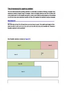
Motivation: Paint shop as bottleneck resource Problem description • Items are set on racks • Each rack has two faces (front and rear) • Two different types of items • Different types may not face each other (“layer constraint”) Target • Minimize needed racks
Problem Type: Special 2D Bin Packing Problem (2DBPP) Markus Seizinger
2
1. Problem Description
Example: Layer Constraint
Front
Rear
Rack Markus Seizinger
3
1. Problem Description
Example: Layer Constraint
Front
Rear
Rack Markus Seizinger
3
1. Problem Description
Example: Layer Constraint
Front
Rear
Rack Markus Seizinger
3
1. Problem Description
Example: Layer Constraint
Front
Rear
Rack Markus Seizinger
3
Agenda 1. Problem Description 2. Bounds 3. Column Generation Algorithm 1. 2. 3.
Master Problem Restricted Master Problem Subproblem Decomposition
4. Computational Study 5. Conclusion and Future Agenda
Markus Seizinger
4
1. Problem Description
Problem Description: 2DBPPLC Items and bins • Set of items 𝑖 ∈ 𝐼 and of item types 𝑡 ∈ 𝑇 • Each item has width 𝑤𝑖 , height ℎ𝑖 , and type 𝑡𝑖 • Every bin is equal with width 𝑊, height 𝐻, and 𝑆 number of layers • No rotation of items allowed Problem task • Assign every item to one bin and assign a concrete position (𝑥|𝑦|𝑧) • Items may not overlap each other or the edges of the bin • Items of different types may not be assigned face to face on the same bin • Objective: Minimize the number of required bins
2DBPP with Layer Constraints (2DBPPLC) Markus Seizinger
5
1. Problem Description
Complexity: 2DBPPLC may be reduced to 2DBPP and 3DBPP
Reduction to 2DBPP
Reduction to 3DBPP
All bins have one layer only, i.e., 𝑆 = 1
Only one type of items exists, i.e., 𝑇 = 1
Regular 2DBPP (strongly NP-hard)
3DBPP, where all items have a size of one at the third dimension Decomposes into 2DBPP (strongly NP-hard)
2DBPPLC is strongly NP-hard Markus Seizinger
6
1. Problem Description
Approaches exist for 2DBPP and 3DBPP Martello & Vigo, 1998, Management Science • Lower Bounds (2DBPP) • Definition of instance classes Martello et al., 2000, Operations Research • Lower Bounds (3DBPP) Lodi et al., 2002a/b, EJOR/Discrete Applied Mathematics • Heuristics (2DBPP) Pisinger & Sigurd, 2007, INFORMS Journal on Computing • CG-based algorithm (2DBPP) • Pre-stage of subproblem with 1DBPP • Updating lower bound with RMP • Valid inequalities Markus Seizinger
7
Agenda 1. Problem Description 2. Bounds 3. Column Generation Algorithm 1. 2. 3.
Master Problem Restricted Master Problem Subproblem Decomposition
4. Computational Study 5. Conclusion and Future Agenda
Markus Seizinger
8
2. Bounds
Upper and lower bounds from literature may be adapted Upper Bounds/Heuristics
Lower Bounds/Relaxations
Adaptation of Extreme Point (EP) packing heuristic • Packs all items as greedy algorithm • EP-selection based on best fit • EP-generation had to be adapted to layer constraints
Adaptation of analytical bounds from literature • L0: Geometric bound • L1: Bound of large items • L2: Hybrid of L0 and L1
• Also used during column generation to pack a single bin
Development of new model-based lower bound 𝑳𝑳𝑪 𝟏𝑫𝑩𝑷 based on 1D-BPP • NP-hard, yet solvable for realistic instances • Dominates all other bounds
Markus Seizinger
9
2. Bounds
Greedy Extreme-Point based Packing Heuristic 𝜋𝑖 𝑖 ℎ𝑖
•
Order items by non-increasing relative value 𝑤
•
Place every item in the best feasible extreme point – –
Extreme points are generated by projecting the upper-right corner of item (w.r.t. type) Best fit rule maximizing type-overlay opposite side
Markus Seizinger
10
2. Bounds
Lower Bounds 𝑳𝟎 - Geometric bound
σ𝑖∈𝐼 𝑤𝑖 ℎ𝑖 𝐿0 = 𝑊⋅𝐻⋅𝑆
𝑳𝟏 - Bound of large items
𝐼
𝑙𝑎𝑟𝑔𝑒
𝑊 𝐻 (𝜏) = {𝑖 ∈ 𝐼: 𝑤𝑖 > ∧ ℎ𝑖 > ∧ 𝜏𝑖 = 𝜏} 2 2
𝐿𝐿𝐶 1
𝐼𝑙𝑎𝑟𝑔𝑒 𝜏 = 𝑆 𝜏∈Τ
Markus Seizinger
11
2. Bounds
Lower Bounds 𝑳𝟐 - Bound of geometry and large items (dominates both 𝐿0 and 𝐿1 )
𝐼1 (𝑝, 𝑞) = {𝑖 ∈ 𝐼: 𝑤𝑖 ≥ 𝑊 − 𝑝 ∧ ℎ𝑖 ≥ 𝐻 − 𝑞} 𝑊 𝐻 𝐼2 𝑝, 𝑞 = {𝑖 ∈ 𝐼 \ 𝐼1 𝑝, 𝑞 : 𝑤𝑖 > ∧ ℎ𝑖 > } 2 2 𝐼3 𝑝, 𝑞 = {𝑖 ∈ 𝐼 \ 𝐼1 𝑝, 𝑞 ∪ 𝐼2 𝑝, 𝑞
𝐿𝐿𝐶 2
=
𝐿𝐿𝐶 1
+
max
𝑊 𝐻 1≤𝑝≤ 2 ; 1≤𝑞≤ 2
0,
: 𝑤𝑖 ≥ 𝑝 ∧ ℎ𝑖 ≥ 𝑞}
σ𝑖∈𝐼2(𝑝,𝑞)∪𝐼3(𝑝,𝑞) 𝑤𝑖 ℎ𝑖 − 𝑆 ⋅ 𝐿1 − 𝐼1 𝑝, 𝑞
⋅𝑊⋅𝐻
𝑊⋅𝐻⋅𝑆
Markus Seizinger
12
2. Bounds
Lower Bounds 𝑳𝟐 - Bound of geometry and large items (dominates both 𝐿0 and 𝐿1 )
𝐼1 (𝑝, 𝑞) = {𝑖 ∈ 𝐼: 𝑤𝑖 ≥ 𝑊 − 𝑝 ∧ ℎ𝑖 ≥ 𝐻 − 𝑞} 𝑊 𝐻 𝐼2 𝑝, 𝑞 = {𝑖 ∈ 𝐼 \ 𝐼1 𝑝, 𝑞 : 𝑤𝑖 > ∧ ℎ𝑖 > } 2 2 𝐼3 𝑝, 𝑞 = {𝑖 ∈ 𝐼 \ 𝐼1 𝑝, 𝑞 ∪ 𝐼2 𝑝, 𝑞
: 𝑤𝑖 ≥ 𝑝 ∧ ℎ𝑖 ≥ 𝑞}
Geometric 𝐿𝐿𝐶 2
=
𝐿𝐿𝐶 1
+
max
𝑊 𝐻 1≤𝑝≤ 2 ; 1≤𝑞≤ 2
0,
Large Items
σ𝑖∈𝐼2(𝑝,𝑞)∪𝐼3(𝑝,𝑞) 𝑤𝑖 ℎ𝑖 − 𝑆 ⋅ 𝐿1 − 𝐼1 𝑝, 𝑞
⋅𝑊⋅𝐻
𝑊⋅𝐻⋅𝑆
Markus Seizinger
12
Agenda 1. Problem Description 2. Bounds 3. Column Generation Algorithm 1. 2. 3.
4. 5. 6. 7.
Master Problem Restricted Master Problem Subproblem Decomposition
Column Generation Computational Study Literature Conclusion and Future Agenda
Markus Seizinger
13
3. Column Generation Algorithm
Solution Approach Master Problem (MP): Set Covering • Requires all feasible packings of items in bins • Choose packings to cover all items • Minimize number of bins
Decomposition and Column Generation • Restricted Master Problem (RMP): Set Covering, as MP, but: – Linearized variables – Only subset of columns Subproblem (SP): 2D Packing Problem with layer constraints • Create attractive packings (see Pisinger & Sigurd, 2007) • Iteratively improves solution of RMP
Markus Seizinger
14
3. Column Generation Algorithm
Linearized Restricted Master Problem (RMP) Number of bins with packing 𝑝
(I)
𝑧 𝑅𝑀𝑃 = min 𝜆𝑝 𝑝∈𝑃
1, if item 𝑖 is included in packing 𝑝
s.t.:
Set of Items
∀𝑖 ∈𝐼
𝑎𝑝𝑖 𝜆𝑝 ≥ 1 𝑝∈𝑃
(II) Set of Packings
∀𝑝 ∈𝑃
𝜆𝑝 ≥ 0
(III)
Note: 𝑃 is a subset of all possible packings Markus Seizinger
15
3. Column Generation Algorithm
Notation: 2D Packing Problem with layer CTs (2DPPLC) Sets, Indices, and Parameters 𝑖∈𝐼 Set of items
𝑡∈𝑇
Set of item types
𝑤𝑖 ℎ𝑖 𝑡𝑖 𝜋𝑖
Width of item 𝑖 Height of item 𝑖 Type of item 𝑖 Dual value of item 𝑖
Decision Variables 𝑥𝑖 x-coordinate of item 𝑖
𝑙𝑖𝑗
1, iff item 𝑖 is placed left of 𝑗
𝑦𝑖
y-coordinate of item 𝑖
𝑏𝑖𝑗
1, iff item 𝑖 is placed below 𝑗
𝑠𝑖
layer of item 𝑖
𝑓𝑖𝑗
1, iff item 𝑖 is placed in front of 𝑗
𝑎𝑖
1, iff item 𝑖 included in bin
𝑊 𝐻 𝑆
Width of bin Height of bin Number of layers
Markus Seizinger
16
3. Column Generation Algorithm
Example: 2D Packing Problem with layer CTs (2DPPLC) 𝑥1 = 0; 𝑥2 = 4; 𝑦1 = 0; 𝑦2 = 5; 𝑠1 = 0; 𝑠2 = 0;
𝑙12 = 0; 𝑙21 = 0; 𝑏12 = 1; 𝑏21 = 0; 𝑓12 = 0; 𝑓21 = 0;
1
Markus Seizinger
17
3. Column Generation Algorithm
Example: 2D Packing Problem with layer CTs (2DPPLC) 𝑥1 = 0; 𝑥2 = 4; 𝑦1 = 0; 𝑦2 = 5; 𝑠1 = 0; 𝑠2 = 0;
𝑙12 = 0; 𝑙21 = 0; 𝑏12 = 1; 𝑏21 = 0; 𝑓12 = 0; 𝑓21 = 0;
2
1
Markus Seizinger
17
3. Column Generation Algorithm
Example: 2D Packing Problem with layer CTs (2DPPLC) 𝑥1 = 0; 𝑥32 = 6; 4; 𝑦1 = 0; 𝑦32 = 5; 𝑠1 = 0; 𝑠32 = 0; 1;
𝑙13 0; 𝑙23 12 = 1; 21 = 0; 𝑏13 12 = 1; 𝑏23 21 = 0; 𝑓13 0; 𝑓23 12 = 1; 21 = 0; 3
1
Markus Seizinger
17
3. Column Generation Algorithm
Model: 2D Packing Problem with layer CTs (2DPPLC) 𝑧 2𝐷𝑃𝑃
=
min 1 − 𝜋𝑖 𝑎𝑖 ⇔ max 𝜋𝑖 𝑎𝑖 𝑖∈𝐼
s.t.: 𝑓𝑖𝑗 + 𝑓𝑗𝑖 + 𝑙𝑖𝑗Items + 𝑙𝑗𝑖 + 𝑏𝑖𝑗 +not 𝑏𝑗𝑖 overlap + 1 − 𝑎𝑖 + 1 − 𝑎𝑗 ≥ may
(I)
𝑖∈𝐼
1
∀ 𝑖, 𝑗 ∈ 𝐼: 𝑖 < 𝑗 ∀ 𝑖, 𝑗 ∈ 𝐼: Items may not 𝑙𝑖𝑗 + 𝑙𝑗𝑖 + 𝑏𝑖𝑗 + 𝑏𝑗𝑖 overlap + 1 − 𝑎𝑖(items + 1 −of𝑎𝑗different ≥ 1 type) 𝑖 < 𝑗 ∧ 𝑡𝑖 ≠ 𝑡𝑗
(II) (III)
𝑥-coordinate
𝑥𝑖 − 𝑥𝑗 + 𝑊𝑙𝑖𝑗
≤
𝑊 − 𝑤𝑖
∀ 𝑖, 𝑗 ∈ 𝐼
(IV)
𝑦-coordinate
𝑦𝑖 − 𝑦𝑗 + 𝐻𝑏𝑖𝑗
≤
𝐻 − ℎ𝑖
∀ 𝑖, 𝑗 ∈ 𝐼
(V)
𝑧-coordinate
𝑠𝑖 − 𝑠𝑗 + S𝑓𝑖𝑗
≤
S−1
∀ 𝑖, 𝑗 ∈ 𝐼
(VI)
Item may not exceed bin (width) 𝑥𝑖 ≤
𝑊 − 𝑤𝑖
∀𝑖 ∈𝐼
(VII)
𝑦𝑖 ≤ Item may not exceed bin (height)
𝐻 − ℎ𝑖
∀𝑖 ∈𝐼
(VIII)
Item may not exceed bin (layers) 𝑠𝑖 ≤
𝐷−1
∀𝑖 ∈𝐼
(IX)
0
∀𝑖 ∈𝐼
(X)
∀ 𝑖, 𝑗 ∈ 𝐼
(XI)
𝑥𝑖 , 𝑦𝑖 , 𝑠𝑖 𝑎𝑖 , 𝑙𝑖𝑗 , 𝑏𝑖𝑗 , 𝑓𝑖𝑗
Markus Seizinger
≥
𝑏𝑖𝑛𝑎𝑟𝑦
18
3. Column Generation Algorithm
Model: 2D Packing Problem with layer CTs (2DPPLC) 𝑧 2𝐷𝑃𝑃
=
min 1 − 𝜋𝑖 𝑎𝑖 ⇔ max 𝜋𝑖 𝑎𝑖 𝑖∈𝐼
s.t.: 𝑓𝑖𝑗 + 𝑓𝑗𝑖 + 𝑙𝑖𝑗 + 𝑙𝑗𝑖 + 𝑏𝑖𝑗 + 𝑏𝑗𝑖 + 1 − 𝑎𝑖 + 1 − 𝑎𝑗 ≥
1
𝑙𝑖𝑗 + 𝑙𝑗𝑖 + 𝑏𝑖𝑗 + 𝑏𝑗𝑖 + 1 − 𝑎𝑖 + 1 − 𝑎𝑗 ≥
1
(I)
𝑖∈𝐼
∀ 𝑖, 𝑗 ∈ 𝐼: 𝑖 < 𝑗 ∀ 𝑖, 𝑗 ∈ 𝐼: 𝑖 < 𝑗 ∧ 𝑡𝑖 ≠ 𝑡𝑗
(II) (III)
𝑥𝑖 − 𝑥𝑗 + 𝑊𝑙𝑖𝑗
≤
𝑊 − 𝑤𝑖
∀ 𝑖, 𝑗 ∈ 𝐼
(IV)
𝑦𝑖 − 𝑦𝑗 + 𝐻𝑏𝑖𝑗
≤
𝐻 − ℎ𝑖
∀ 𝑖, 𝑗 ∈ 𝐼
(V)
𝑠𝑖 − 𝑠𝑗 + S𝑓𝑖𝑗
≤
S−1
∀ 𝑖, 𝑗 ∈ 𝐼
(VI)
𝑥𝑖
≤
𝑊 − 𝑤𝑖
∀𝑖 ∈𝐼
(VII)
𝑦𝑖
≤
𝐻 − ℎ𝑖
∀𝑖 ∈𝐼
(VIII)
𝑠𝑖
≤
𝐷−1
∀𝑖 ∈𝐼
(IX)
𝑥𝑖 , 𝑦𝑖 , 𝑠𝑖
≥
0
∀𝑖 ∈𝐼
(X)
∀ 𝑖, 𝑗 ∈ 𝐼
(XI)
𝑎𝑖 , 𝑙𝑖𝑗 , 𝑏𝑖𝑗 , 𝑓𝑖𝑗
Markus Seizinger
𝑏𝑖𝑛𝑎𝑟𝑦
18
3. Column Generation Algorithm RMP: Restricted Master Problem 2DPPLC: 2D Packing Problem w. layer CTs
Iteration scheme Dual values 𝜋
RMP
2DPPLC
New packing Markus Seizinger
19
3. Column Generation Algorithm
Problems: 2D Packing Problem with layer CTs (2DPPLC) Re-formulation
Selection Algorithm
Current problems • Number of decision variables rises exponentially to 𝐼 • Excessive runtime for realistic problem instances
1. Exclude items with non-positive duals
Alternate approach (Fekete et al. 2007) • Reduces symmetries • Finding special interval graphs • Tree search algorithm • But: no good results as well
3. Apply 1D Knapsack Problem (1DKPLC) as pre-stage • 1DKP with layer constraints • Solution time < 0.1s • Pre-selected items
2. Create start solution based on heuristics
Markus Seizinger
20
3. Column Generation Algorithm RMP: Restricted Master Problem 1DKPLC: 1D Knapsack Problem w. layer CTs 2DPPLC: 2D Packing Problem w. layer CTs
Iteration scheme Dual values 𝜋
1DKPLC
RMP
Item subset
2DPPLC
New packing Markus Seizinger
21
3. Column Generation Algorithm RMP: Restricted Master Problem 1DKPLC: 1D Knapsack Problem w. layer CTs 2DPPLC: 2D Packing Problem w. layer CTs
Iteration scheme Dual values 𝜋
1DKPLC
RMP
Forbid previous subset
Item subset
2DPPLC
New packing Markus Seizinger
21
3. Column Generation Algorithm
Dominating items A dominated item 𝑗 can not be part of the optimal packing unless all of it’s dominating items 𝑖 are packed as well. Definition 𝑖≽𝑗⟺ 𝑤𝑖 ≤ 𝑤𝑗 ∧ ℎ𝑖 ≤ ℎ𝑗 ∧ 𝜋𝑖 ≥ 𝜋𝑗 ∧ 𝑡𝑖 = 𝑡𝑗 𝑖≻𝑗 ⟺ 𝑖 ≽ 𝑗 ∧ (𝑤𝑖 < 𝑤𝑗 ∨ ℎ𝑖 < ℎ𝑗 ∨ 𝜋𝑖 > 𝜋𝑗 ) Implied constraints 𝑥𝑖 ≥ 𝑥𝑗
∀ 𝑖, 𝑗 ∈ 𝐼: 𝑖 ≻ 𝑗
Markus Seizinger
22
3. Column Generation Algorithm
Conflicting items ሚ that are in strict (weak) conflict can not be packed on the same A set of items 𝐶 (𝐶) bin (layer) We process weak conflicts in preprocessing and check whether or not pairs of two and groups of three items can be possibly be packed. Strict conflicts are created by taking item types into account. Implied constraints 𝑎𝑖
≤
𝐶 −1
∀𝐶 ∈𝒞
𝑖∈𝐶
𝑓𝑖𝑗
≥
1
∀ 𝐶ሚ ∈ 𝒞ሚ
ሚ 𝑖,𝑗∈𝐶:𝑖≠𝑗
Markus Seizinger
23
3. Column Generation Algorithm
Strengthened model: 2DPPLC 𝑧 2𝐷𝑃𝑃
=
min 1 − 𝜋𝑖 𝑎𝑖 ⇔ max 𝜋𝑖 𝑎𝑖 𝑖∈𝐼
(I)
𝑖∈𝐼
s.t.: …
…
…
𝑥𝑖
≥
𝑥𝑗
𝑎𝑖
≤
Item dominances
Strict conflicts
𝐶 −1
(II-IX) ∀ 𝑖, 𝑗 ∈ 𝐼: 𝑖 ≻ 𝑗
(X)
∀𝐶 ∈𝒞
(XI)
𝑖∈𝐶
Weak conflicts
𝑓𝑖𝑗
≥
1
∀ 𝐶ሚ ∈ 𝒞ሚ
(XII)
𝑥𝑖 , 𝑦𝑖 , 𝑠𝑖
≥
0
∀𝑖 ∈𝐼
(XIII)
∀ 𝑖, 𝑗 ∈ 𝐼
(XIV)
ሚ 𝑖,𝑗∈𝐶:𝑖≠𝑗
𝑎𝑖 , 𝑙𝑖𝑗 , 𝑏𝑖𝑗 , 𝑓𝑖𝑗
Markus Seizinger
𝑏𝑖𝑛𝑎𝑟𝑦
24
3. Column Generation Algorithm
Strengthened model: 2DPPLC 𝑧 2𝐷𝑃𝑃
=
min 1 − 𝜋𝑖 𝑎𝑖 ⇔ max 𝜋𝑖 𝑎𝑖 𝑖∈𝐼
(I)
𝑖∈𝐼
s.t.:
Strict conflicts
…
…
…
𝑥𝑖
≥
𝑥𝑗
𝑎𝑖
≤
𝐶 −1
(II-IX) ∀ 𝑖, 𝑗 ∈ 𝐼: 𝑖 ≻ 𝑗
(X)
∀𝐶 ∈𝒞
(XI)
𝑖∈𝐶
Weak conflicts
𝑓𝑖𝑗
≥
1
∀ 𝐶ሚ ∈ 𝒞ሚ
(XII)
𝑥𝑖 , 𝑦𝑖 , 𝑠𝑖
≥
0
∀𝑖 ∈𝐼
(XIII)
∀ 𝑖, 𝑗 ∈ 𝐼
(XIV)
ሚ 𝑖,𝑗∈𝐶:𝑖≠𝑗
𝑎𝑖 , 𝑙𝑖𝑗 , 𝑏𝑖𝑗 , 𝑓𝑖𝑗
Markus Seizinger
𝑏𝑖𝑛𝑎𝑟𝑦
24
3. Column Generation Algorithm
Strengthened model: 2DPPLC 𝑧 2𝐷𝑃𝑃
=
min 1 − 𝜋𝑖 𝑎𝑖 ⇔ max 𝜋𝑖 𝑎𝑖 𝑖∈𝐼
(I)
𝑖∈𝐼
s.t.: …
…
…
𝑥𝑖
≥
𝑥𝑗
𝑎𝑖
≤
𝐶 −1
(II-IX) ∀ 𝑖, 𝑗 ∈ 𝐼: 𝑖 ≻ 𝑗
(X)
∀𝐶 ∈𝒞
(XI)
𝑖∈𝐶
𝑓𝑖𝑗
≥
1
∀ 𝐶ሚ ∈ 𝒞ሚ
(XII)
𝑥𝑖 , 𝑦𝑖 , 𝑠𝑖
≥
0
∀𝑖 ∈𝐼
(XIII)
∀ 𝑖, 𝑗 ∈ 𝐼
(XIV)
ሚ 𝑖,𝑗∈𝐶:𝑖≠𝑗
𝑎𝑖 , 𝑙𝑖𝑗 , 𝑏𝑖𝑗 , 𝑓𝑖𝑗
Markus Seizinger
𝑏𝑖𝑛𝑎𝑟𝑦
24
Agenda 1. Problem Description 2. Bounds 3. Column Generation Algorithm 1. 2. 3.
Master Problem Restricted Master Problem Subproblem Decomposition
4. Computational Study 5. Conclusion and Future Agenda
Markus Seizinger
25
4. Computational Study
Instance Classes of Martello & Vigo (1998) 4 Classes of items –
Dimensions of items are uniformly distributed in an interval (depending on it‘s class) 2. High items
1. Wide items –
𝑤𝑖 ∈
2 3
𝑊; 𝑊 ; ℎ𝑖 ∈ 1;
𝐻 2
;
𝑤𝑖 ∈
𝑊 2
+ 1; 𝑊 ; ℎ𝑖 ∈
𝑤𝑖 ∈ 1;
𝑊 2
; ℎ𝑖 ∈
2 3
𝐻; 𝐻 ;
4. Small items
3. Large items –
–
𝐻 2
+ 1; 𝐻 ;
–
𝑤𝑖 ∈ 1;
𝑊 2
; ℎ𝑖 ∈ 1;
𝐻 2
;
4 Classes of instances • Instance (𝑥) contains 70% class 𝑥 items and 10% of every other item class 2 Subclasses • A: Types are equally distributed over all items • B: For instance (𝑥) all items of class 𝑥 are of the same type
Markus Seizinger
26
4. Computational Study
Instance Classes Instance class|subclass
1|A
“Wide items” 2 𝑊, 𝑊 3 1 ℎ𝑖 ~𝑈 1, 𝐻 2
𝑤𝑖 ~ 𝑈
35 %
1|B
70 %
2|A
5%
2|B 3|A
5%
3|B 4|A 4|B
35 %
“High items” 1 𝑤𝑖 ~ 𝑈 1, 𝑊 2
ℎ𝑖 ~𝑈
5%
3
𝐻, 𝐻
5%
1 𝑊 + 1, 𝑊 2 1 ℎ𝑖 ~𝑈 𝐻 + 1, 𝐻 2
𝑤𝑖 ~ 𝑈
5%
10 % 5%
35 %
10 %
70 %
5%
5%
10 % 5%
2
“Large items”
5% 10 %
5%
35 %
5%
“Small items” 1 𝑤𝑖 ~ 𝑈 1, 𝑊 2 1 ℎ𝑖 ~𝑈 1, 𝐻 2
5%
10 % 5%
5%
10 % 5%
10 % 5%
35 %
10 %
70 %
5%
5%
10 %
Markus Seizinger
35 %
5%
5% 10 %
5%
5% 10 %
5%
35 %
10 %
70 %
35 %
27
4. Computational Study
Setup Instances • 10 instances of every combination of class (4), subclass (2), and number of items (5) randomly generated • Total of 400 instances • 𝑊 = 𝐻 = 10; 𝑆 = 2; 𝛵 = 2
BFDH: Best-fit decreasing height algorithm L0: Geometric bound L1: Bound of large items L2: Hybrid of L0 and L1 𝐿𝐿𝐶 1𝐷𝐵𝑃 : Model-based lower bound
Initialization • Initial columns generated by BFDH-LC algorithm • Lower bounds 𝐿0 , 𝐿1 , and 𝐿2 • 𝐿𝐿𝐶 1𝐷𝐵𝑃 with runtime limit of ten minutes (if reached, best lower bound is used) Column Generation • Total runtime limited to five hours • Terminated when root node relaxation was solved Markus Seizinger
28
4. Computational Study BFDH: Best-fit decreasing height algorithm 𝐿𝐿𝐶 1𝐷𝐵𝑃 : Model-based lower bound
Bounds Analytical Bound
L0: Geometric bound L1: Bound of large items L2: Hybrid of L0 and L1
Model-Based
Class
Size
𝐿0
𝐿1
𝐿2
𝐿1𝐷𝐵𝑃
BFDH Algo.
abs. Gap
rel. Gap
#optimal
1|A 1|A 1|A 1|A 1|A 1|B 1|B 1|B 1|B 1|B 2|A 2|A 2|A 2|A 2|A 2|B 2|B 2|B 2|B 2|B
20 40 60 80 100 20 40 60 80 100 20 40 60 80 100 20 40 60 80 100
3,3 6,0 8,6 11,4 14,3 3,3 6,0 8,6 11,4 14,3 3,3 6,1 8,6 11,3 13,8 3,3 6,1 8,6 11,3 13,8
1,0 2,0 2,5 3,3 3,8 0,9 1,7 2,5 3,1 3,6 1,0 2,0 2,5 3,3 3,8 0,9 1,7 2,5 3,1 3,6
3,3 6,0 8,6 11,4 14,3 3,3 6,0 8,6 11,4 14,3 3,3 6,1 8,6 11,3 13,8 3,3 6,1 8,6 11,3 13,8
3,3 6,0 8,6 11,4 14,3 3,5 6,1 8,6 11,4 14,3 3,3 6,1 8,6 11,3 13,8 3,7 6,1 8,6 11,3 13,8
3,9 7,2 10,1 13,2 16,6 4,0 7,1 10,3 13,6 16,8 4,2 7,3 10,2 13,0 15,8 4,2 6,8 10,3 13,5 16,0
0,6 1,2 1,5 1,8 2,3 0,5 1,0 1,7 2,2 2,5 0,9 1,2 1,6 1,7 2,0 0,5 0,7 1,7 2,2 2,2
19% 20% 17% 16% 16% 16% 17% 20% 19% 17% 28% 20% 19% 15% 15% 14% 12% 20% 20% 16%
4 1 0 0 0 5 0 0 0 0 1 0 0 0 0 5 3 0 0 0
Markus Seizinger
29
4. Computational Study BFDH: Best-fit decreasing height algorithm 𝐿𝐿𝐶 1𝐷𝐵𝑃 : Model-based lower bound
Bounds Analytical Bound
L0: Geometric bound L1: Bound of large items L2: Hybrid of L0 and L1
Model-Based
Class
Size
𝐿0
𝐿1
𝐿2
𝐿1𝐷𝐵𝑃
BFDH Algo.
abs. Gap
rel. Gap
#optimal
3|A 3|A 3|A 3|A 3|A 3|B 3|B 3|B 3|B 3|B 4|A 4|A 4|A 4|A 4|A 4|B 4|B 4|B 4|B 4|B
20 40 60 80 100 20 40 60 80 100 20 40 60 80 100 20 40 60 80 100
5,2 9,9 14,7 19,0 24,0 5,2 9,9 14,7 19,0 24,0 2,3 4,0 5,8 7,3 8,9 2,3 4,0 5,8 7,3 8,9
6,1 11,2 16,0 21,1 26,9 6,0 11,1 15,5 20,8 26,7 1,2 2,1 2,5 3,4 4,2 1,1 1,9 2,3 3,1 3,9
6,8 13,2 18,4 24,8 31,1 6,8 13,2 18,4 24,8 31,1 2,3 4,0 5,8 7,3 8,9 2,3 4,0 5,8 7,3 8,9
7,2 13,3 18,4 24,8 31,1 7,2 13,3 18,4 24,8 31,1 2,4 4,0 5,8 7,3 8,9 2,4 4,0 5,8 7,3 8,9
7,6 13,8 19,4 25,8 32,5 7,8 14,3 19,9 26,6 33,7 2,8 4,7 6,4 8,1 9,8 2,9 4,8 6,6 8,1 10,1
0,4 0,5 1,0 1,0 1,4 0,6 1,0 1,5 1,8 2,6 0,4 0,7 0,6 0,8 0,9 0,5 0,8 0,8 0,8 1,2
6% 4% 5% 4% 5% 8% 8% 8% 7% 8% 20% 18% 11% 11% 10% 22% 21% 13% 11% 14%
6 6 2 0 0 4 2 0 0 0 6 3 4 2 1 5 3 2 3 0
Markus Seizinger
30
4. Computational Study
Key Results •
𝐿0 is equal for pairs of subclasses X|A and X|B –
•
Item dimensions are not influenced by subclass
BFDH: Best-fit decreasing height algorithm L0: Geometric bound L1: Bound of large items L2: Hybrid of L0 and L1 𝐿𝐿𝐶 1𝐷𝐵𝑃 : Model-based lower bound
𝐿1 does differ for pairs of subclasses X|A and X|B – –
Bound can take item types explicitly into account 𝐿𝐴1 ≥ 𝐿𝐵1
•
𝐿2 can improve 𝐿0 and 𝐿1 , if difference between these both bounds is small
•
Model-based bound 𝐿𝑆𝐶 1𝐷𝐵𝑃 dominates all other bounds
•
Relative gap is not significantly influenced by instance size
•
Mostly small instances could be solved to optimality by BFDH algorithm
Markus Seizinger
31
4. Computational Study
Column Generation All instances Class Size #instances
1|A 20 1|A 40 1|A 60 1|A 80 1|A 100 1|B 20 1|B 40 1|B 60 1|B 80 1|B 100 2|A 20 2|A 40 2|A 60 2|A 80 2|A 100 2|B 20 2|B 40 2|B 60 2|B 80 2|B 100
10 10 10 10 10 10 10 10 10 10 10 10 10 10 10 10 10 10 10 10
Succesfully terminated
time #columns #instances
0:18 4:07 5:00 4:46 5:00 0:10 3:44 4:22 4:25 5:00 0:34 3:23 4:20 4:56 5:00 0:00 1:58 4:56 4:40 5:00
40 268 591 904 1280 52 247 451 865 1411 86 366 667 1100 1096 26 138 517 820 816
10 4 0 2 0 10 4 3 2 0 10 5 3 1 0 10 7 1 2 0
#LB #UB time #columns improved improved
0:18 2:47
40 220
3:51
1121
0:10 1:50 2:54 2:06
52 206 470 904
0:34 1:46 2:49 4:20
86 245 841 319
0:00 0:40 4:24 3:20
26 102 1231 900
Markus Seizinger
3 2 0 2 0 2 3 4 3 0 4 4 2 1 0 0 2 0 2 0
2 2 0 0 0 2 0 1 2 0 5 4 1 0 0 4 2 4 3 1
CG LB
CG UB
3,6 6,2 8,6 11,7 14,3 3,7 6,4 9,1 11,9 14,3 3,7 6,5 8,8 11,5 13,8 3,7 6,4 8,6 11,6 13,9
3,7 7,0 10,1 13,2 16,6 3,8 7,1 10,2 13,4 16,8 3,7 6,9 10,1 13,0 15,7 3,8 6,6 9,9 13,2 16,0
initial LB initial UB
3,3 6,0 8,6 11,4 14,3 3,5 6,1 8,6 11,4 14,3 3,3 6,1 8,6 11,3 13,8 3,7 6,1 8,6 11,3 13,9
3,9 7,2 10,1 13,2 16,6 4,0 7,1 10,3 13,6 16,8 4,2 7,3 10,2 13,0 15,7 4,2 6,8 10,3 13,5 16,1 32
4. Computational Study
Column Generation All instances Class Size #instances
3|A 20 3|A 40 3|A 60 3|A 80 3|A 100 3|B 20 3|B 40 3|B 60 3|B 80 3|B 100 4|A 20 4|A 40 4|A 60 4|A 80 4|A 100 4|B 20 4|B 40 4|B 60 4|B 80 4|B 100
10 10 10 10 10 10 10 10 10 10 10 10 10 10 10 10 10 10 10 10
Succesfully terminated
time #columns #instances
0:00 0:00 1:57 1:36 3:31 0:00 0:01 3:09 1:01 2:47 0:01 2:27 3:54 3:55 4:26 0:02 3:10 2:44 3:25 5:00
6 7 27 36 38 4 21 54 66 67 30 1014 1415 2454 2001 45 857 587 1785 2554
10 10 7 8 5 10 10 4 9 6 10 7 4 3 1 10 6 6 4 0
#LB #UB time #columns improved improved
0:00 0:00 0:39 0:45 2:20 0:00 0:01 0:24 0:35 1:41 0:01 1:22 2:16 1:23 0:00 0:02 1:58 1:13 1:03
6 7 28 34 35 4 21 49 66 60 30 614 0 950 0 45 535 544 716
Markus Seizinger
1 2 6 5 6 0 2 6 8 6 2 2 0 1 0 2 1 4 1 0
1 1 3 0 0 5 7 5 5 8 1 2 0 0 0 3 2 1 0 0
CG LB
CG UB
7,3 13,5 19,0 25,3 32,1 7,2 13,5 19,0 25,6 32,0 2,6 4,2 5,8 7,4 8,9 2,6 4,1 6,2 7,4 8,9
7,5 13,7 19,1 25,8 32,8 7,3 13,6 19,3 26,0 33,1 2,7 4,5 6,4 8,1 9,8 2,6 4,6 6,5 8,1 10,1
initial LB initial UB
7,2 13,3 18,4 24,8 31,3 7,2 13,3 18,4 24,8 31,3 2,4 4,0 5,8 7,3 8,9 2,4 4,0 5,8 7,3 8,9
7,6 13,8 19,4 25,8 32,8 7,8 14,3 19,9 26,6 34,0 2,8 4,7 6,4 8,1 9,8 2,9 4,8 6,6 8,1 10,1 33
4. Computational Study
Key Results •
Results for classes 1|A, 1|B, 2|A, 2|B similar –
•
Best results could be achieved for 3|A and 3|B – –
•
Problem structure is closely related
Only few columns needed to terminate Termination criterion could be found fast
4|A and 4|B are hardest instances – –
Most columns generated, mainly by packing heuristic Hard to prove no new negative reduced-cost column exists
•
Last iteration not solvable
•
Using heuristic as warm-start speeds up subproblem dramatically
Markus Seizinger
34
Agenda 1. Problem Description 2. Bounds 3. Column Generation Algorithm 1. 2. 3.
Master Problem Restricted Master Problem Subproblem Decomposition
4. Computational Study 5. Conclusion and Future Agenda
Markus Seizinger
35
5. Conclusion and Future Agenda
Conclusion Problem class • 2DBP with layer constraints has never been published • No effective exact methods for 2DBP with layer constraints known Solution approach • Decomposition necessary • Column generation serves to provide an additional lower bound • Convergence of column generation quite bad Problems • Hard to prove that no new negative reduced cost column exists • Speed of subproblem is limiting factor
Markus Seizinger
36
5. Conclusion and Future Agenda
Future Agenda Improve subproblem formulation • Reduce symmetries • Provide better lower bounds • Restrict packing to certain Guillotine Cuts
Evaluate Constraint Satisfaction Approach • CP-solvers might find infeasible packings faster • Layer constraints restrict possible domains of pairs of items Graph representation of packing • Check results of Fekete et al. • Special interval graphs are equivalent to packings • Easy to adapt formulation to apply to layer constraints
Markus Seizinger
37
Questions and comments!
Markus Seizinger
38
(1/2)
Graphs representing feasible packings 4
“Translating” packings to a set of graphs • One graph 𝐺𝑖 for every dimension 𝑖 • An edge 𝑎𝑏 exists in 𝐺𝑖 exists, iff projections of items 𝑎 and 𝑏 overlap in dimension 𝑖
𝑖=1
3 2 1
6
5
𝑖=2 1
1
6
2
6
2
5
3
5
3
4
4 Markus Seizinger
39
(2/2)
Graphs representing feasible packings N
𝑖=1
𝑖=2 1
1
6
2
6
2
5
3
5
3
4
4 Markus Seizinger
40
(2/2)
Graphs representing feasible packings N : 𝐸 𝑖 =∅
𝑖=1 2 𝐸 𝑖 =∅
for Edges 𝐸 𝑖 connecting to vertices of different type
𝑃4:
ځ2𝑖=1 𝐸𝑖 = ∅
for Edges 𝐸𝑖 connecting to vertices of different type
𝑖=1
𝑖=2 1
1
6
2
6
2
5
3
5
3
4
4 Markus Seizinger
40
(1/2)
1DBPPLC as lower bound Sets, Indices, and Parameters 𝑖∈𝐼 Set of items 𝜏∈Τ Set of item types 𝑊 𝐻
Width of bin Height of bin
𝑠∈𝑆 𝑏∈𝐵
Set of bin layers Set of bins
𝑤𝑖 ℎ𝑖 𝜏𝑖
Width of item 𝑖 Height of item 𝑖 Type of item 𝑖
Additional Sets and Expressions 𝐼ሚ𝑖 = 𝑖 ′ |𝑖 ′ ∈ 𝐼: ℎ𝑖 + ℎ𝑖 ′ > 𝐻 ∧ 𝑤𝑖 + 𝑤𝑖 ′ > 𝑊 ∧ 𝑖 ≠ 𝑖 ′ 𝐼𝑖ҧ = 𝑖 ′ |𝑖 ′ ∈ 𝐼ሚ𝑖 : 𝜏𝑖 ≠ 𝜏𝑖 ′
Set of conflicting items for 𝑖
𝐴ҧ𝜏𝑏𝑠 = σ𝑖∈𝐼𝜏 𝑤𝑖 ℎ𝑖 𝑥𝑖𝑏𝑠
Area used by items of type 𝜏
Set of conf. items of diff. type
Decision Variables 𝑥𝑖𝑏𝑠 1, iff item 𝑖 is assigned to layer 𝑠 of bin 𝑏 𝑦𝑏 1, iff bin 𝑏 is used 41
(2/2)
1DBPPLC as lower bound 𝐿𝑆𝐶 1𝐷𝐵𝑃
=
min 𝑦𝑏
(I)
𝑏∈𝐵
𝑠. 𝑡. :
𝑥𝑖𝑏𝑠
=
1
∀𝑖 ∈𝐼
(II)
𝑥𝑖𝑏𝑠 − 𝑦𝑏
≤
0
∀ 𝑖 ∈ 𝐼, 𝑏 ∈ 𝐵, 𝑠 ∈ 𝑆
(III)
𝑤𝑖 ℎ𝑖 𝑥𝑖𝑏𝑠
≤
𝑊𝐻
∀ 𝑏 ∈ 𝐵, 𝑠 ∈ 𝑆
(IV)
≤
𝑊𝐻
∀𝑏 ∈ 𝐵, 𝑠, 𝑠′ ∈ 𝑆, 𝜏 ∈ T
(V)
𝑥𝑖𝑏𝑠 + 𝑥𝑖 ′ 𝑏𝑠
≤
1
(VI)
𝑥𝑖𝑏𝑠 + 𝑥𝑖 ′ 𝑏𝑠′
≤
1
∀ 𝑖 ∈ 𝐼, 𝑖 ′ ∈ 𝐼ሚ𝑖 , 𝑏 ∈ 𝐵, 𝑠 ∈ 𝑆 ∀ 𝑖 ∈ 𝐼, 𝑖 ′ ∈ 𝐼𝑖ҧ , 𝑏 ∈ 𝐵, 𝑠, 𝑠′ ∈ 𝑆
(VII)
𝑏∈𝐵 𝑠∈𝑆
𝑖∈𝐼
𝐴ҧ𝜏𝑏𝑠 +
𝐴ҧ𝜏′ 𝑏𝑠′ 𝜏′ ∈Τ\{𝜏}
𝑥𝑖𝑏𝑠
𝑏𝑜𝑜𝑙𝑒𝑎𝑛
∀𝑖 ∈ 𝐼, 𝑏 ∈ 𝐵, 𝑠 ∈ 𝑆
(VIII)
𝑦𝑏
𝑏𝑜𝑜𝑙𝑒𝑎𝑛
∀𝑏 ∈𝐵
(IX) 42
(1/2)
1DKPLC as pre-stage Sets, Indices, and Parameters 𝑖∈𝐼 Set of items 𝑊 𝐻 𝐷= 𝑆
Width of bin Height of bin Number of Layers
𝑡∈𝑇
Set of item types
𝑤𝑖 ℎ𝑖 𝑡𝑖 𝜋𝑖
Width of item 𝑖 Height of item 𝑖 Type of item 𝑖 Dual value of item 𝑖
Additional Sets and Expressions 𝐼ሚ𝑖 = 𝑖 ′ |𝑖 ′ ∈ 𝐼: ℎ𝑖 + ℎ𝑖 ′ > 𝐻 ∧ 𝑤𝑖 + 𝑤𝑖 ′ > 𝑊 ∧ 𝑖 ≠ 𝑖 ′ 𝐼𝑖ҧ = 𝑖 ′ |𝑖 ′ ∈ 𝐼ሚ𝑖 : 𝜏𝑖 ≠ 𝜏𝑖 ′ 𝐴ҧ𝜏𝑠 = σ𝑖∈𝐼𝜏 𝑤𝑖 ℎ𝑖 𝑥𝑖𝑠
Set of conflicting items for 𝑖 Set of conf. items of diff. type
Area used by items of type 𝜏 on layer 𝑠
Decision Variables 𝑥𝑖𝑠 1, iff item 𝑖 is placed on layer 𝑠 of bin 𝑎𝑖 1, iff item 𝑖 is placed in bin 43
(2/2)
1DKPLC as pre-stage 𝑧1𝐷𝐾𝑃
=
min 1 − 𝜋𝑖 𝑎𝑖
(𝐼)
𝑖∈𝐼
𝑥𝑖𝑠
𝑠. 𝑡. :
=
𝑎𝑖
∀𝑖 ∈𝐼
(𝐼𝐼)
≤
𝑊𝐻
∀𝑠 ∈𝑆
(𝐼𝐼𝐼)
≤
𝑊𝐻
∀ 𝑠, 𝑠′ ∈ 𝑆, 𝜏 ∈ T
(𝐼𝑉)
𝑥𝑖
≥
𝑥𝑗
(𝑉)
𝑥𝑖𝑠 + 𝑥𝑖 ′ 𝑠
≤
1
∀ 𝑖, 𝑗 ∈ 𝐼: 𝑖 ≻ 𝑗 ∀ 𝑖 ∈ 𝐼, 𝑖 ′ ∈ 𝐼ሚ𝑖 , 𝑠 ∈ 𝑆
𝑥𝑖𝑠 + 𝑥𝑖 ′ 𝑠′
≤
1
∀ 𝑖 ∈ 𝐼, 𝑖 ′ ∈ 𝐼𝑖ҧ , 𝑠, 𝑠′ ∈ 𝑆
𝑠∈𝑆
𝑤𝑖 ℎ𝑖 𝑥𝑖𝑠 𝑖∈𝐼
𝐴ҧ𝜏𝑠 +
𝐴ҧ𝜏′𝑠′ 𝜏′ ∈Τ\{𝜏}
𝑥𝑖𝑠
𝑏𝑖𝑛𝑎𝑟𝑦
∀ 𝑖 ∈ 𝐼, 𝑠 ∈ 𝑆
𝑎𝑖
𝑏𝑖𝑛𝑎𝑟𝑦
∀𝑖 ∈𝐼
(𝑉𝐼) (𝑉𝐼𝐼) (𝑉𝐼𝐼𝐼)
(IX) 44
(1/3)
2D Packing Problem with layer CTs (2DPPLC) Sets, Indices, and Parameters 𝑖∈𝐼 Set of items 𝑡∈𝑇 Set of item types
s∈𝑆
layers of bin
𝑤𝑖 ℎ𝑖 𝑡𝑖 𝜋𝑖
Width of item 𝑖 Height of item 𝑖 Type of item 𝑖 Dual value of item 𝑖
Decision Variables 𝑥𝑖 x-coordinate of item 𝑖 𝑠𝑖 layer of item 𝑖
𝑦𝑖 𝑎𝑖
y-coordinate of item 𝑖 1, iff item 𝑖 is placed in bin
𝑙𝑖𝑗
1, iff item 𝑖 is placed left of 𝑗
𝑏𝑖𝑗
1, iff item 𝑖 is placed below 𝑗
𝑓𝑖𝑗
1, iff item 𝑖 is placed in front of 𝑗
𝑊 𝐻 𝐷= 𝑆
Width of bin Height of bin Number of layers
Markus Seizinger
45
(2/3)
Model: 2D Packing Problem with layer CTs (2DPPLC) 𝑧 2𝐷𝑃𝑃
=
min 1 − 𝜋𝑖 𝑎𝑖 ⇔ max 𝜋𝑖 𝑎𝑖 𝑖∈𝐼
s.t.: 𝑓𝑖𝑗 + 𝑓𝑗𝑖 + 𝑙𝑖𝑗 + 𝑙𝑗𝑖 + 𝑏𝑖𝑗 + 𝑏𝑗𝑖 + 1 − 𝑎𝑖 + 1 − 𝑎𝑗 ≥
1
𝑙𝑖𝑗 + 𝑙𝑗𝑖 + 𝑏𝑖𝑗 + 𝑏𝑗𝑖 + 1 − 𝑎𝑖 + 1 − 𝑎𝑗 ≥
1
(I)
𝑖∈𝐼
∀ 𝑖, 𝑗 ∈ 𝐼: 𝑖 < 𝑗 ∀ 𝑖, 𝑗 ∈ 𝐼: 𝑖 < 𝑗 ∧ 𝑡𝑖 ≠ 𝑡𝑗
(II) (III)
𝑥𝑖 − 𝑥𝑗 + 𝑊𝑙𝑖𝑗
≤
𝑊 − 𝑤𝑖
∀ 𝑖, 𝑗 ∈ 𝐼
(IV)
𝑦𝑖 − 𝑦𝑗 + 𝐻𝑏𝑖𝑗
≤
𝐻 − ℎ𝑖
∀ 𝑖, 𝑗 ∈ 𝐼
(V)
𝑠𝑖 − 𝑠𝑗 + S𝑓𝑖𝑗
≤
S−1
∀ 𝑖, 𝑗 ∈ 𝐼
(VI)
𝑥𝑖
≤
𝑊 − 𝑤𝑖
∀𝑖 ∈𝐼
(VII)
𝑦𝑖
≤
𝐻 − ℎ𝑖
∀𝑖 ∈𝐼
(VIII)
𝑠𝑖
≤
𝐷−1
∀𝑖 ∈𝐼
(IX)
𝑥𝑖
≥
𝑥𝑗
∀ 𝑖, 𝑗 ∈ 𝐼: 𝑖 ≻ 𝑗
(X)
𝑥𝑖 , 𝑦𝑖 , 𝑠𝑖
≥
0
∀𝑖 ∈𝐼
(XI)
∀ 𝑖, 𝑗 ∈ 𝐼
(XII)
𝑎𝑖 , 𝑙𝑖𝑗 , 𝑏𝑖𝑗 , 𝑓𝑖𝑗 Markus Seizinger
𝑏𝑖𝑛𝑎𝑟𝑦
46
(3/3)
2DPPLC (B) 𝑧 2𝐷𝑃𝑃
=
min 1 − 𝜋𝑖 𝑎𝑖
(I)
𝑖∈𝐼
𝑥𝑖𝛼𝛽𝑠
𝑠. 𝑡. :
=
𝑎𝑖
=
0
∀𝑖 ∈𝐼
(II)
𝛼∈Α 𝛽∈Β 𝑠∈𝑆
𝑥𝑖𝛼𝛽𝑠
𝑀 𝑥𝑖𝛼𝛽𝑏𝑠 − 1 +
𝑖 ′ ∈𝐼\𝐼 ′ (𝜏𝑖 ) 𝛼 ′ ∈Α′
𝑖,𝑖 ′ ,𝛼
𝛽 ′ ∈Β′
𝑖,𝑖 ′ ,𝛽
(III)
𝑥𝑖 ′ 𝛼 ′ 𝛽 ′ 𝑠
≤
1
∀ 𝑖 ∈ 𝐼, 𝛼 ∈ Α, 𝛽 ∈ Β, 𝑠 ∈ 𝑆
(𝐼𝑉)
𝑥𝑖 ′ 𝛼 ′ 𝛽 ′ 𝑠 ′
≤
0
∀ 𝑖 ∈ 𝐼, 𝛼 ∈ Α, 𝛽 ∈ Β, 𝑠 ∈ 𝑆
(𝑉)
∀ 𝑖 ∈ 𝐼, 𝛼 ∈ Α, 𝛽 ∈ Β, 𝑠 ∈ 𝑆
(𝑉𝐼)
𝑖 ′ ∈𝐼 𝛼 ′ ∈Α′ 𝑖,𝑖 ′ ,𝛼 𝛽 ′ ∈Β′ 𝑖,𝑖 ′ ,𝛽
𝑀 𝑥𝑖𝛼𝛽𝑏𝑠 − 1 +
∀ 𝑖 ∈ 𝐼, 𝛼 ∈ Α, 𝛽 ∈ Β, 𝑠 ∈ 𝑆: 𝛼 + 𝑤𝑖 > 𝑊 ∨ 𝛽 + ℎ𝑖 > 𝐻
𝑠 ′ ∈𝑆\{𝑠}
𝑥𝑖𝛼𝛽𝑠
𝑏𝑖𝑛𝑎𝑟𝑦
𝑎𝑖
𝑏𝑖𝑛𝑎𝑟𝑦
Markus Seizinger
∀𝑖 ∈𝐼
(𝑉𝐼𝐼) 47