3. irrigation scheduling - Science Direct

Microirrigation for Crop Production F.R. Lamm, J.E. Ayars and F.S. Nakayama (Editors) © 2007 Elsevier B.V. All rights reserved.

61

3. IRRIGATION SCHEDULING TERRY A. HOWELL USDA-ARS, Bushland, Texas, USA “Good is the enemy of great.” Jim Collins

MOSHE MERON MIGAL Galilee Technological Center, Kiryat Shmona, ISRAEL “The art of irrigation is manipulation of soil water content to achieve desired plant responses."

3.1. INTRODUCTION Irrigation scheduling generally determines the time of the next event and the amount of water to apply. For microirrigation this is the decision of when to start an irrigation cycle and how long to irrigate the zone or set. Scheduling microirrigation is inherently different from other irrigation methods because the application amount per irrigation is small and the applications are typically more frequent. Martin et al. (1990), Heermann et al. (1990), and Hill (1991) provide a thorough discussion of irrigation scheduling principles. This chapter covers principles and application techniques applicable to microirrigation systems. Microirrigation scheduling integrates elements of the system hydraulic design and maintenance together with various aspects of the soil and the crop characteristics with the atmospheric evaporative demand. It involves providing managers with the irrigation needs of the crop that must be organized together with the cultural aspects of growing and harvesting the crop. Microirrigation scheduling is often integrated into the system controls through automation (see Chapter 7). Irrigation scheduling involves long-term decisions (strategic) and short-term decisions (tactical) that must consider the producers’ risks and management goals in harmony with the agronomic or horticultural requirements for the crops being grown across the irrigation block, field, farm, or even across a broader scheme (i.e., irrigation district or hydrologic basin). Because microirrigation has a relatively high investment cost, it is more often used on higher valued crops and with water supplies designed to meet the peak crop water use rates. Microirrigation scheduling is generally controlled by (1) measuring or estimating crop water needs, (2) measuring a soil water status, or (3) measuring a plant water status property. The latter two conditions are frequently used to determine irrigation needs and are easily integrated into an automated control system (Phene et al., 1990). The former, traditionally, has been used through an evapotranspiration-water balance model and is adaptable to both indicating the need as well as the amount of water that should be applied (Jensen et al., 1990; Allen et al., 1998). Other factors influencing the scheduling of microirrigation systems may include soil salinity, impact of water deficits on crop quality, or the impact of rain on salt leaching into the root zone.

62

MICROIRRIGATION FOR CROP PRODUCTION

3.1.1. System Capacity System capacity, Sc, is a critical design and operational parameter. System capacity is typically expressed as the ratio of the system flowrate (Q in m3 s-1) to the land area (A in m2), resulting in units of m s-1. It is typically more convenient to express the ratio in units of mm d-1 as follows:

Sc (m s-1 ) =

Q (m3 s-1 ) 86.4 x 106 Q (m3 s-1 ) -1 or S (mm d ) = c A (m2 ) A (m2 )

(3.1)

When expressed by the second equation of Eq. 3.1, Sc is in equivalent units to daily evapotranspiration rates, and commonly used units for the system application rate. Sc becomes a direct index useful in determining the irrigation scheduling flexibility to meet the crop needs, time available for system maintenance, time available for cultural needs, and time available to recover from equipment failures. Sc must exceed the peak evapotranspiration rate less any dependable short-term effective precipitation to provide the necessary ability to meet the crop water use rate with minimal soil water depletion and to meet other non-operational periods required for maintenance and routine repairs or equipment replacement. Sc should not exceed a system application rate that is greater than the ability of the soil to infiltrate adequately the applied water. 3.1.2. System Uniformity Effects on Scheduling Irrigation systems cannot apply water uniformly across an irrigation set or field due to inherent variabilities in soil hydraulic properties (see Chapter 2), soil topography, and system hydraulics (see Chapter 5 and Chapter 10). For microirrigation, emitter flow variations from clogging may need to be considered as well (Nakayama and Bucks, 1981). In addition, each of these factors will vary temporally and spatially and may not always be statistically independent of each other. Many estimation methods have been used to characterize the application variations for microirrigation systems (Tab. 3.1). Initially, microirrigation system flow variations were characterized using technology adopted from sprinkler irrigation. Two such parameters are the Christiansen uniformity coefficient, Cu (Christiansen, 1942), and the distribution uniformity, Du, of the low quarter of the field taken from surface irrigation that was used by the USDA-NRCS (formerly the USDA-Soil Conservation Service) since the late 1940s (Kruse, 1978; and Merriam and Keller, 1978). For microirrigation, the emitter flowrate was often used in the Cu and Du computations rather than the application amount or the amount infiltrated because it was easier to measure. Table 1 indicates the similarity of many of these measures. Hart (1961) demonstrated that the Christiansen Cu for a normal distribution of application amounts was a function of the coefficient of variation (Cv, σ / x ; where σ is the standard deviation and x is the mean). The Hart Cu is often called the HSPA (Hawaiian Sugar Planter’s Association) Cu. Because microirrigation systems often have more than one emission device per plant, Keller and Karmeli (1975) derived the design emission uniformity (Eu) based on the low quarter flow distribution uniformity (Du), the emitter manufacturing flow variability, the number of emitters per plant, and the ratio of minimum to mean emitter flow. Solomon and Keller (1978) illustrated the impact of increased Cvm (manufacturing coefficient of variability) on decreased uniformity. Nakayama et al. (1979) derived a design coefficient of uniformity (Cud) based on the

3. IRRIGATION SCHEDULING

63

average emitter flowrate for microirrigation. Both Eu and Cud indicate an improvement when the number of emission devices (with the same manufacturing Cvm) is increased per plant. Of course, the investment cost will increase with a greater number of emitters per plant. Microirrigation uniformity increases, nearly proportionally, with lower Cvm values indicating the importance of precision in the manufacturing. Bucks et al. (1982) classified Cvm values and presented recommended ranges for Eu and Cud for arid areas. Wu and Gitlin (1977) used the emitter flow variation, qvar, defined as 1 - (qn / qm ), where qn is the minimum emitter flowrate and qm is the maximum emitter flowrate. Warrick (1983) evaluated Cu and Du for six assumed statistical distributions and found no effect of the statistical distribution for small values of Cv < 0.25, as would likely occur for many microirrigation systems. He demonstrated that approximate values of Cu and Du each depended mainly on the Cv of the distribution and that a unique relationship existed between Du and Cu (see Tab. 3.1). Table 3.1 Examples characterizing irrigation application variations Term Cu

Reference

Equation

Christiansen (1942)

Cu = [1 - ( Σ| x - x | ) / Σx]

HSPA Cu Hart (1961)

HSPA Cu = [1 - (2/π)1/2 (Cv)]

Eu

Keller & Karmeli (1975)

Eu = [1 - 1.27 (Cvm) n-1/2] (qn / q )

CUd

Nakayama et al. (1979)

Cud = [1 - 0.798 (Cvm) n-1/2]

Du

Kruse (1978); Merriam and Keller (1978)

Du = x lq / x

qvar

Wu and Gitlin (1977)

qvar = [1 - (qn / qm )

DU*

Warrick (1983)

Du* = 1 - 1.3 Cv or Du* = -0.6 + 1.6 Cu* [Note: Du* is for Cv < 0.25]

x - individual emitter application rate x - mean of “N” samples for emitter application rates Cv - coefficient of variation (σ / x; where σ is the sample standard deviation in flow) Cvm - manufacturer’s coefficient of variation n - number of emitter per plant qn - minimum emitter application rate (typically at the minimum pressure) - mean emitter application rate q xlq - mean emitter application rate for the lowest 25% (low quarter) of the emitters qm - maximum emitter application rate NOTE: All terms expressed as decimal fractions and (2/π)0.5 = 0.798. Bralts et al. (1981) illustrated that the hydraulic flow variability was sufficiently independent of the flow variation from manufacturing for single-chamber microirrigation tubing that the total coefficient of flow variability (Cvt) could be expressed as

64

Cvt =


( Cvh

2

+ Cvm 2 )

(3.2)

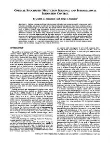
where Cvh is the coefficient of variation in emitter flow due to hydraulic factors. However, when the Cvh exceeded 15%, Clemmens (1987) and Wu et al. (1985) found that Eq. 3.2 under predicted the total flow variation, which was attributed to departure from the assumed normal distribution. Clemmens and Solomon (1997) developed a generalized procedure to estimate the distribution uniformity for any fractional area of the field together with methods for defining the confidence interval of the result. An example of microirrigation application distributions for a mean amount of 10 mm with Cu values of 0.76, 0.84, and 0.92 for an assumed normal distribution with the resulting Cv values of 0.3, 0.2, and 0.1, respectively, is presented in Fig. 3.1. This illustration highlights the within irrigation set or field variations in applications that could affect measurements of soil or plant water status affecting irrigation scheduling and water management. The spread in amounts is particularly noticeable as the Cu declined from 0.92 to 0.84 or lower. Bucks et al. (1982) reported measured Cv values for eight emitters that ranged from 0.06 to 0.15 from initial laboratory measurements, and the values increased substantially in some cases, just four years later by up to 400% based on field measurements. Their results varied by emitter design and depended on water treatment techniques for the Colorado River water used in their study. Nakayama and Bucks (1981) observed significantly reduced uniformity when only 1 to 5% of the emitters were clogged even with 2 to 8 emitters per plant. These in-field performances would further skew the applications and greatly reduce irrigation uniformity and efficiency. Although emitter flow uniformity is important in microirrigation, the goal remains to apply the necessary water to each plant. The soil (see Chapter 2) and the plant roots dictate the success in meeting this goal in combination with the irrigation system. The soil water properties, the crop rooting characteristics, and the irrigation system uniformity all affect irrigation scheduling decisions with microirrigation to a larger extent than with other irrigation methods. This is because not all the soil surface is wetted and the soil wetting and crop root water extraction patterns are three dimensional in most cases. 3.1.3. System Maintenance Effects on Scheduling The heart of microirrigation success lies in system maintenance (see Chapter 11) and management. System maintenance begins with the design (see Chapter 5) and installation and continues with routine system performance and evaluation (Chapter 10). These are integral procedures of system management, and therefore, directly related to irrigation scheduling. As with irrigation scheduling, system maintenance has long-term (strategic) components that include off-season repairs and checks, and short-term (tactical) components such as recording water flowmeters, pressure gages, fertilizer injections, water treatment chemical injections, and routine filter and line flushing. Often these tactical maintenance operations can be automated by computerized controllers. Water flowmeters and pressure gauges are critical components of the system and must be included in the system installation. These measurement devices provide critical feedback data needed for irrigation scheduling. Similarly, successful irrigation scheduling must include the


65

time requirements to maintain and calibrate water treatment equipment, fertilizer or other agrochemical injection equipment, the time needed to clean or backflush filters, and the time to flush mainlines, submains, and lateral lines. Time will be needed for tactical emergency equipment repairs and replacements. Preventative maintenance will likely minimize this, but equipment failures are impossible to forecast even in the best situation. Most operational maintenance and management (filter backflushing, flowmeter and pressure gauge observations) can be performed while the system is operating. However, some operations (e.g., screen washing, line flushing) will require additional time when the system is not operating. The water supply quality (biological, chemical, and physical) will greatly impact filtration design and operational needs. Management plans must consider the time estimates for these operations in addition to the normal time requirements for irrigation as governed by system capacity.

Figure 3.1. Diagram illustrating variability of applied water for a mean application of 10 mm for Cu values varying from 0.92 to 0.76.

3.1.4. Scheduling Constraints Many operational, agronomic, or horticultural cultural practices require time that cannot be used for irrigating, and thus, increase the required irrigation design capacity. Fortunately with microirrigation, many tasks can be performed simultaneously with the irrigation (e.g., applying fertilizer or spraying the crop or orchard). The principal constraints to irrigation scheduling of microirrigation systems are the available water flowrate, and in some cases the available water volume or amount, and the water delivery schedule. The simplest case is a sole-source supply such as a well or a dedicated reservoir. With a well, the groundwater formation basically determines the well yield (flowrate) and its draw down (dynamic pumping lift). With a reservoir, its location determines the pumping lift, and its volume and water supply determine the sustained yield (flowrate). In most cases, some regulations may apply to these water sources, and permits or laws may restrict the pumping rate or pumping volume.

66


More commonly, irrigation supplies may be shared water resources. Often in these cases, the water may only be available on a set or prior request basis. Depending on the exact circumstances, the grower may need to provide a surface reservoir to supply a demand-based microirrigation system. The energy supply may become a constraint. Unless the supply reservoir or canal is sufficiently higher than the irrigated field, some type of water pumping system is required with microirrigation systems. For many systems, centrifugal pumps are used that generally require priming. If priming is required, automation is more difficult. In addition, energy supplies may be controlled or regulated to curtail peak summer demand loads on electrical generating plants requiring pumps to be idled or turned off during certain hours.

3.2. IRRIGATION SCHEDULING TECHNIQUES Microirrigation systems are routinely scheduled for irrigations using either (a) a demand system based on knowing or predicting the crop water needs, (b) a soil-water control feedback or feedforward system that measures soil water contents in the root zone, or (c) a plant-water-status control system based on measuring the crop water status. Obviously, these different methods of irrigation scheduling can be used simultaneously, but often labor or equipment may limit that approach. The grower should view each system as providing information rather than an exact answer. This information can then be weighted along with their experience to determine the irrigation needs of the crop. The latter method has long been used based on crop appearance and the experience of the grower. The soil water system could be as simple as manually coring or spading into the root zone to observe the soil wetness by feel. The demand-based system can be based on relatively simple criteria such as historical records or evaporation pans to more complex and extensive computer models using elaborate weather station equipment. Regardless of the method used, several considerations must be evaluated: •

ease of integration into the farm or horticultural management

•

labor, equipment, technology, and capital required to implement the system(s)

• •

accuracy and reliability of the system(s) ability to forecast irrigation needs

•

ability to identify problem areas in an irrigation set or a field

•

ability to adjust and handle seasonal temporal and spatial changes

•

ability to monitor the irrigation system performance

More than one of these scheduling methods may be required to handle these considerations. 3.2.1 Water Balance (Evapotranspiration Base) The water balance approach is based on ascertaining the water inputs and water outflows from the field. It is best described as a checkbook approach with irrigations and rainfall as the deposits, and evapotranspiration (ET, crop water use) as the main withdrawal. Percolation beneath the crop root zone could be considered as a service fee or a necessary expense to control salinity. Based on this analogy, the soil water becomes the bank (or checkbook) balance, where the grower tries to maintain a minimum balance to avoid endangering the crop yield or quality without exceeding a maximum amount that might not be insured against loss from runoff or


67

drainage beneath the root zone. When the available soil water declines too low or reaches the minimum account balance, the crop will suffer a stress that will reduce ET and perhaps yield. The one-dimensional water balance equation is

θ z i+ 1 = θ z i + (Pi - Q ro i )+ I n i - E Ti - D z i

(3.3)

where θzi is the soil water content on day i integrated over the root zone depth z, P is rainfall, Qro is runoff, In is net applied irrigation, ET is crop water use from the root zone, and Dz is deep percolation beneath the root zone at depth z. Dz is generally negative as indicated in Eq. 3.3, but it could be positive if water moved upward from a shallow water table. Each term in Eq. 3.3 is expressed in water depth units (mm), and P, Qro, and In are at the soil surface. ET is considered as the sum of evaporation (E) from plant or soil surfaces and transpiration (T) is from the plant leaves. The term, P- Qro, is the effective precipitation or the amount of the precipitation that would be expected to infiltrate into the root zone. Similarly, In is usually taken as the amount of “net” irrigation, which is the gross irrigation amount multiplied by the irrigation application efficiency. Each term will vary spatially and temporally (Gardner, 1960), so that in practice the mean values must be assumed due to the difficulty in determining the spatial distribution of the terms. The one-dimensional water balance expressed by Eq. 3.3, although widely used in microirrigation, requires careful integration and measurement of the terms to approximate the three-dimensional patterns expected in microirrigation. Runoff (Qro) is particularly difficult to estimate. Fortunately, losses to Qro from microirrigation applications are usually minimal; however, Qro losses from rainfall can be significant in some cases even with a partially dry soil surface that is characteristic of microirrigation applications. Williams (1991) describes runoff models used in EPIC (erosion productivity impact calculator) (Williams et al., 1983) that could estimate rainfall runoff. The precipitation, P, that strikes the plant canopy will be intercepted by the leaves and stems and then distributed in relation to the canopy architecture (e.g., trees at the canopy edge, corn at the stem). This makes estimating P in orchards and vineyards that reaches the ground (throughfall) difficult to estimate accurately over the plant spatial ground area. E and T losses will be discussed in more detail in the succeeding sections. Losses to Dz are also difficult to estimate, but they are likely to approach one-dimensional flow patterns near the rootzone bottom (Hillel, 1998). Deep percolation, Dz, below a 1.4-m soil depth was greater for driplines spaced 2.3 and 3.1 m than for a 1.5-m spacing for subsurface drip irrigated corn on a silt loam soil in Kansas (Darusman et al., 1997a). In a related study at the same location, Darusman et al. (1997b) determined that Dz was significant for subsurface drip-irrigated corn when inseason irrigations exceeded about 400 mm. For in-season irrigations that were less than 300 mm, they determined that about 20 mm of water moved into the root zone from upward capillary flow. Richards et al. (1956) showed that the decrease in soil water content occurred inversely proportional to time as Dz = -

dθ = -a t -b dt

(3.4)

where θ is the soil water content in mm and a and b are empirical constants related to the boundary conditions and the soil hydraulic conductivity, K(θ). Assuming an exponential function between K(θ) and θ, Hillel (1998) demonstrated that Dz was equal to K(θ) for gravity drainage alone at θz at the bottom of the root zone.

68


Shallow groundwater tables can provide significant water to a crop depending on the water table depth, the groundwater salinity, and the crop rooting characteristics. Wallender et al. (1979) reported that cotton extracted up to 60% of its ET from a saline (6 dS m-1) perched water table, and Ayars and Schoneman (1986) that cotton extracted up to 37% of its ET from a more saline water table (10 dS m-1), but irrigation management greatly affected the groundwater uptake. Ayars and Hutmacher (1994) demonstrated a practical approach for managing irrigations over a shallow (1.2 to 2 m), moderately saline (5 dS m-1) perched water table that permitted 25% of the ET from groundwater without any adverse effects on crop growth or yield. Cotton can use water from a water table as deep as 2.7 m even under a favorable irrigation regime (Namken et al.,1969). Kruse et al. (1993) found that alfalfa used saline or nonsaline water from shallow water tables in its first year, but that a salinity buildup reduced yields with saline water tables in subsequent years. Corn and wheat were less affected by the salinity, but the crops used less water from a 1.0-m water table. Upward water flowrates into the crop root zone from water tables 2 to 4 m deep were predicted to range from 2 to 6 mm d-1 by Doorenbos and Pruitt (1977). Soppe and Ayars (2003) measured groundwater use exceeding 3 mm d-1 from a shallow, saline (14 dS m-1) water table by safflower with groundwater contributing up to 40% of the daily water use. 3.2.1.1. Climatic factors affecting crop water use Weather parameters directly influence crop water use (Allen et al., 1998). The principal factors are solar irradiance (Rs), air temperature (Ta), relative humidity (RH) or air dew point temperature (Td), barometric pressure (Pb), and wind speed (U). Solar irradiance is reduced to net radiation (Rn), which is the main solar factor affecting crop water use, as follows: R n = (1 - α ) R s - R nl

(3.5)

where α is the albedo or short-wave reflection (fraction) and Rnl is net long-wave radiation. The albedo of most crops will be about 0.20 to 0.23, whereas the soil albedo will be less, about 0.1 to 0.15 depending on the soil and its water content. The net long-wave radiation term depends on several surface and atmospheric parameters. Basically, long-wave radiation is proportional to the surface temperature to the fourth power times the surface emissivity and a proportionality constant known as the Stefan-Boltzman factor. A perfect emitting surface has an emissivity of 1.0. The emissivity of most soils and crops is near 0.98, while the emissivity of the sky is much lower and will depend on the atmospheric water content. Because the sky emissivity and the sky temperature are not routinely measured, Rnl is estimated using routine air temperature data, relative humidity data, and estimates of cloud cover (Allen et al., 1998). The weather parameters at or over the crop affect its water use. However, it is largely impractical to measure weather parameters over the crop, except for research, so weather parameters are typically measured at a weather station situated to represent the crop environment. Although many organizations have attempted to standardize the weather station siting and the instrumentation, in most cases this is difficult to achieve. Allen et al. (1998) discusses the impact of the station siting, instrument maintenance, and other factors on the quality of weather data for estimating crop water use. Although many equations can estimate crop water use based on climatic data, the Penman (1948) combination equation has become widely used. It is expressed as


ETo =

[ Δ (Rn -G )] + [( γ W f ) (eo s - ea )] [ λ ρ w (Δ+γ )]

69

(3.6)

where ETo is the ET of grass that is well-watered and fully covering the soil in mm d-1, Δ is the slope of the saturated vapor pressure curve at the mean air temperature in kPa °C-1, G is the heat flux into the soil in MJ m-2 d-1, γ is the psychrometric constant in kPa °C-1, Wf is an empirical wind function in MJ m-2 d-1 kPa-1 [Wf = 6.43 + (3.453 U2), where U2 is the mean daily wind speed in m s-1 at 2.0 m height over grass], eo s is the saturated vapor pressure at the mean daily air temperature in kPa, ea is the mean ambient vapor pressure in kPa, λ is the latent heat of vaporization in MJ kg-1, and ρw is water density (1.0 Mg m-3). For irrigated grass with a full cover, daily G is approximately zero MJ m-2 d-1. The psychrometric constant, γ, is proportional to barometric pressure, which is inversely related to elevation. The Penman equation was not widely used initially because it was rather complex for its time (before calculators/computers), and it was difficult to compute all the parameters and find locations with the necessary meteorological data. Despite these drawbacks, Van Bavel (1956) recognized its potential and its conservative nature as well as its usefulness for determining water use from large areas with nonlimiting soil water and for estimating the irrigation need. Monteith (1965) characterized the empirical wind function using the atmospheric aerodynamic resistance (ra in s m-1) and added a bulk surface resistance term (rs in s m-1), which resulted in the following equation:

ETo =

[Δ ( Rn - G )] + [(86.4 ρ C p ) ( es - ea ) / ra ] [λ ρw ( Δ + γ *)]

(3.7)

where ρ is air density in kg m-3, Cp is the specific heat of moist air [1.013 kJ kg-1 °C-1], es is the mean saturated vapor pressure at the daily maximum and minimum air temperature in kPa, and an adjusted psychrometric constant, γ* = γ (1 + rs / ra) in kPa °C-1. Table 3.2 gives the recommended equations for estimating the parameters along with the appropriate constants for grass from Allen et al. (1998) and Allen et al. (1994). Jensen et al. (1990) recommended two standardized reference surfaces, 0.12-m for tall grass and 0.5-m tall for alfalfa. They recommended rs be set to 45 s m-1 for alfalfa and to 70 s m-1 for grass. The resulting functions for defining ra (in s m-1) using air temperature and humidity data from a 2.0-m height were 110 / U2 and 208 / U2, respectively, for alfalfa and grass. Allen et al. (1998) used only a grass reference equation and simplified the parameters in Eq. 3.7 to the following: 900 U 2 (es - ea )] (Tma + 273) ρ w [ Δ + γ (1 + 0.34 U 2 )]

[ 0.408 (Rn -G )] + [ γ ETo =

(3.8)

where Tma is mean daily air temperature at 2 m in °C. For a day (24 h), G in Eq. 3.8 can be assumed to be zero MJ m-2 d-1. Equation 3.8 (also known as the FAO Penman-Monteith Eq.) is the recommended method for calculating world-wide standard grass reference ET ( FAO-56, Food and Agriculture Organization of the United Nations), replacing FAO-24 (Doorenbos and Pruitt, 1977) that was also based on a grass reference, but that required empirical correction factors for humidity, wind speed, and day to night wind speed variations (Frevert et al., 1983).

70


Table 3.2. Equations for estimating parameters in the Penman and Penman-Monteith equations for grass reference ET (ETo) from Allen et al. (1998); (1994). Term

Unit o

Tma λ Pb γ eo(Tma) es ea Δ G dr δ ωs Ra Rso TminK TmaxK Rnl Rns Rn TK TvK ρ Cp rs LAI d ZoM ZoH ra

C MJ kg-1 kPa kPa oC-1 kPa kPa kPa kPa oC-1 MJ m-2 d-1 radians radians radians MJ m-2 d-1 MJ m-2 d-1 K K MJ m-2 d-1 MJ m-2 d-1 MJ m-2 d-1 K K kg m-3 kJ kg-1 oC-1 s m-1 – m m m s m-1

γ*

kPa oC-1

Equation (Tmin + Tmax)/2 2.501 - (2.361 x 10-3) T or assume λ = 2.45 101.3 [(293 - 0.0065 z) / 293]5.26 0.00163 Pb / λ 0.6108 exp [(17.27 Tma) / (Tma + 237.3)] [eo (Tmin) + eo (Tmax)]/2 0.6108 exp [(17.27 Tdew) / (Tdew + 237.3)] 4098 {0.6108 exp [(17.27 Tma) / (Tma+ 237.3)]} / (Tma+ 237.3)2 0.0 [for a day or 24 hr] 1 + 0.033 cos[(2 π J) / 365] 0.409 sin[(2 π J) / 365) - 1.39] arcos[-tan(ν) tan(δ)] [(1440 Gc dr) / π] [ωs sin(ν) sin(δ) + cos(ν) cos(δ) sin(ωs)] (0.75 + 2 x 10-5 z) Ra Tmin + 273.16 Tmax + 273.16 σ [(TminK + TmaxK) / 2] (0.34 - 0.14 ea1/2)[1.35 - 0.35 (Rs / Rso)] (1 - 0.23) Rs Rns - Rnl Tma + 273.16 TK [1 - 0.378 (ed / Pb)]-1 3.486 (Pb / TvK ) 1.013 rl / (0.5 LAI) or 70 for 0.12-m tall grass 24 hc (2/3) hc 0.123 hc 0.0123 hc {ln[(Zm - d)/ZoM] ln [(Zh - d)/ZoH]} / (k2 Uz) or 208 / U2 for Zm and Zh = 2.0 m for 0.12-m tall grass γ [1 + (rs / ra )] γ (1 + 0.34 U2)


71

Table 3.2. Equations for estimating parameters in the Penman and Penman-Monteith equations for grass reference ET (ETo) from Allen et al. (1998); (1994). Cont. Tmin Tmax Tdew z dr J δ ωs ν Ra Gc Rso Rs TminK TmaxK Rnl σ Rns Rn TK TvK rl LAI hc Zm Zh k Uz U2

-

minimum daily air temperature, oC maximum daily air temperature, oC mean daily dew point temperature, oC elevation above sea level, m inverse relative distance Earth to the Sun, radians integer day of year solar declination angle, radians sunset hour angle, radians latitude, radians daily extraterrestrial radiation, MJ m-2 d-1 solar constant [0.0820 MJ m-2 min-1] clear sky daily solar irradiance, MJ m-2 d-1 daily solar irradiance, MJ m-2 d-1 minimum daily absolute air temperature, K maximum daily absolute air temperature, K net outgoing long-wave radiation, MJ m-2 d-1 Stefan-Boltzman constant [4.903 x10-9 MJ m-2 K-4 d-1] net short-wave radiation, MJ m-2 d-1 net radiation, MJ m-2 d-1 mean daily absolute temperature, K virtual absolute temperature, K leaf resistance, s m-1 [100 s m-1] leaf area index grass height, m [0.12 m] measurement height of wind speed, m [usually2 m] measurement height of air humidity, m [usually 2 m] von Karman constant [0.41] mean daily wind speed at height Zm, m s-1 mean daily wind speed at 2 m, m s-1

3.2.1.2. Crop factors affecting ET Several crop factors were mentioned in the previous section. These include the short-wave reflection (α, albedo) and long-wave emissivity (ε) that affect net radiation and the partitioning of solar irradiance into the various energy balance terms. Two crop architectural characteristics, crop height (hc) and leaf area index (LAI), affect crop water use in various manners. Both parameters are important in determining the soil cover by the crop that affects solar radiation penetration to the ground which in turn affects the sensible energy entering or leaving the ground as soil heat flux. Crop height is an important factor in determining the aerodynamic resistance of the canopy (ra) to latent and sensible heat flux. Leaf area index largely determines the amount of plant foliage exposed to the direct solar irradiance and the amount of shaded plant foliage exposed to transmitted and reflected diffuse solar radiation. Usually, taller crops will have a lower ra value and a higher water use rate for similar surface resistance (rs) values. Typically, a

72


LAI value between 3 and 4 (three to four times the leaf area of one side of the leaves per unit ground area) will be sufficient to maximize transpiration and fully shade the ground. The plant species largely determines the leaf stomatal resistance to water vapor transfer and carbon dioxide uptake. Generally, the type of photosynthetic pathway in the plant species (either C3, C4, or CAM) affects the leaf surface resistance to water vapor transport through the leaf stomata that determines the leaf resistance (rl). The leaf resistance, fraction of shaded and sunlit leaves, and the LAI largely determine the canopy surface resistance (rs). Crop development and growth processes change both of these key crop parameters (hc, and LAI) that determine the water use potential of the crop (Fig. 3.2). Perennial plant species have different annual growth cycles. In most cases for trees or vines, the annual change in height may be small and limbs may even be removed through pruning. These species will have a distinct leaf and fruit bearing cycle. Nondestructive light interception or simple ground-cover measurements are often used instead of measured LAIs for trees and vines because the LAI measurements are difficult to make.

6

4 Leaf Area Index Crop Height

3

4

2

2

1

Crop Height, m

Leaf Area Index

8

Full-Season Corn Source: Howell et al. (1998)

0 0 120 140 160 180 200 220 240 260 280

Day of Year - 1994 Figure 3.2. Leaf area index and crop height of irrigated corn at Bushland, Texas illustrating typical crop development rates (Howell et al., 1998). Allen et al. (1998) provides two methods for estimating the crop effects on water use based on the computed grass reference ETo (Eq. 3.8). These are designated as the single (Kc) and dual (Kcb) crop coefficient approaches based on E T = K c (E T o ) E T = (K c b + K e ) E T o

(3.9) (3.10)


73

where ET represents the crop water use for both soil and plant water evaporation (E) and plant transpiration (T); Kcb is the basal crop coefficient when the soil surface is visually dry (Wright, 1982), but the crop transpiration is not restricted by soil water deficits; and Ke is the coefficient representing the soil water evaporation from a wet soil surface. By examining Eqs. 3.9 and 3.10, ones sees that the single crop coefficient is simply equated to Kcb + Ke, and for a visually dry soil surface case, Kc equals Kcb. In principle, ETo normalizes the evaporative demand of the atmosphere. However, because ETo represents a short, smooth crop that is well watered, the grass water use may be different from that of a real crop or orchard / vineyard. The crop coefficients, Kc or Kcb + Ke, are designed to make the transformation in water use from the idealized standard grass represented by the characteristics embodied in Eq. 3.8 to the real crop. Any of the preceding crop characteristics, albedo, emissivity, height, surface resistance, and the degree of soil wetness and soil salinity of the root zone (to be discussed in the next section) can affect Kc. The single Kc approach assumes a more generalized approach in determining the crop water use that cannot account for some of the soil factors embodied in the dual Kcb approach, especially different soil water evaporation rates that may be important with microirrigation. Equations 3.9 and 3.10 predict crop water use under standard conditions. It is thought to be an upper envelope (Allen et al., 1998) representing conditions without limits on crop growth or water use from a soil water deficit, with normal crop density, with healthy plants without disease or insect damage, without weeds, and without soil salinity effects on crop growth or water use. The Kc and Kcb values are temporally dependent on the crop growth characteristics (hc and LAI) that affect the real crop’s ra and rs values. The idealized Kc and Kcb crop curves for wine grape are illustrated for standard crop development rates in Fig. 3.3.

Figure 3.3. Example of seasonal crop coefficient curve for wine grape representing the major crop growth periods – initial development, crop development (developing ground cover), mid season (reproduction, fruiting, etc.), and late season (maturation and harvest). The heavy line with the circle points is the Kc curve, and the lighter line with the square points is the Kcb curve. Adapted from Allen et al. (1998).

74


Allen et al. (1998) summarized and presented a vast list of Kc and Kcb values based on defining the annual crop development cycle into its initial phase (planting, emergence, early growth), crop developmental phase (rapid vegetative growth, early reproductive development), mid-season phase (full-canopy development, reproductive phases, fruiting, bloom, pollination, early maturation), and ending phase (senescence, fruit maturity, grain filling, dry down). Tables 3.3 through 3.5 adapted from Allen et al. (1998) give Kc and Kcb values for several crops that are often microirrigated. They provide appropriate crop growth stage length periods (L) for the initial (sub “ini”), crop development (sub “dev”), mid season (sub “mid”), and the end of season (sub “end”) growth phases that can be used to construct seasonal crop growth curves as the example in Fig. 3.3. Extended treatment with greater in-depth descriptions and specific details about these values, and data for crops not listed here is given by Allen et al. (1998). They also discuss and review procedures for developing crop coefficients for locations and crops not listed in Allen et al. (1998) or Doorenbos and Pruitt (1977).

Percent of Mature Orchard ET

Fereres and Goldhamer (1990) presented mid-season crop coefficients for a grass reference ET for deciduous fruit and nut trees. They also discussed prior literature reporting crop coefficients considerably larger than the more common maximum Kc value of around 1.20 for denselypopulated peach and pecan trees. Fereres et al., (1981a) reported that micro-advection in young developing orchards from the large amount of surrounding non-evaporating bare soil had small differences in ET compared with the more mature orchards once the younger orchards developed about 50 to 60% ground cover. The ET of young microirrigated almond orchards was dependent on irrigation frequency and the soil wetting patterns (see next section in this chapter), but it was highly related to the area of the ground shaded by the trees at noon (Fereres et al., 1982) (Fig. 3.4). Close agreement was found between estimates of evapotranspiration for young almond trees calculated using mature orchard crop coefficients (Eq. 3.9 and 3.10) as modified by the shaded-area percentage (Fig 3.4) and those obtained through using extensive soil water balance measurements (Sharples et al., 1985). 100 1- to 4-yr old trees 6-yr old trees

80 60 40

Microirrigated Almond Trees

20 0

0

10

20

30

40

50

Percent Shaded Area Figure 3.4. Relationship between shaded area and ET for young almond trees relative to ET from a mature almond orchard. Data were obtained from 1- to 4-yr old trees (circles) and 6-y old trees (squares) using soil water balance methods. Adapted from Fereres et al., 1982.


75

Table 3.3. Vegetable and tuber Kc and basal Kcb values and length of typical growth stages (days) with planting dates and their regions. Adapted from Allen et al. (1998). Kc ini Kc mid Kc end Plant Crop Kcb ini Kcb mid Kcb end Region date Lini Lmid Lend Ldev 0.70 1.05 0.90 0.15 1.00 0.80 Bell pepper 25/30 35 40 20 April/June Mediterranean 30 40 110 30 October Arid 0.70 1.05 0.95 Broccoli 0.15 0.95 0.85 35 45 40 15 September California, USA 0.70 1.05 0.95 Cabbage 0.15 0.95 0.85 40 60 50 15 September California, USA 0.50 0.85 0.60 0.15 0.75 0.50 Cantaloupe 30 45 35 10 January California, USA 10 60 25 25 August California, USA 0.70 1.05 0.95 0.15 0.95 0.85 Carrot 30 50 90 30 October. California, USA 30 40 60 20 Feb./Mar. Mediterranean 0.70 1.05 0.95 Cauliflower 0.15 0.95 0.85 35 50 40 15 September California, USA 0.70 1.05 1.00 0.15 0.95 0.90 Celery 25 40 95 20 October Arid 25 40 45 15 April Mediterranean 0.70 1.00 0.95 0.15 0.90 0.90 Lettuce 20 30 15 10 April Mediterranean 30 45 25 10 Nov./Jan. Mediterranean 25 35 30 10 Oct./Nov. Arid 0.70 1.05 0.75 0.15 0.95 0.65 Onion (dry) 20 35 110 45 Oct./Jan. Arid 15 25 70 40 April Mediterranean 0.70 1.00 1.00 0.15 0.90 0.90 Onion (green) 25 30 10 5 April/May Mediterranean 30 55 55 40 March California, USA

76


Table 3.3. Vegetable and tuber Kc and basal Kcb values and length of typical growth stages (days) with planting dates and their regions. Adapted from Allen et al. (1998). Continued. Kc ini Kc mid Kc end Plant Crop Region Kcb ini Kcb mid Kcb end date Ldev Lini Lmid Lend 0.50 1.15 0.75 0.15 1.10 0.65 Potato 25 30 45 30 May Continental 45 30 70 25 April/May Idaho, USA 0.50 1.00 0.80 Pumpkin 0.15 0.95 0.70 20 30 30 20 Mar., Aug. Mediterranean 0.50 0.95 0.75 0.15 0.90 0.70 Squash 25 35 25 15 Apr., Dec. Mediterr., Arid 20 30 25 15 May/June Mediterr., Europe 0.50 1.05 0.75 0.15 1.00 0.70 Sweet melon 25 35 40 20 May Mediterranean 30 30 50 30 March California, USA 0.50 1.15 0.65 Sweet potato 0.15 1.10 0.55 20 30 60 40 April Mediterranean 0.70 1.15 0.7-0.9 0.15 1.10 0.6-0.8 Tomato 35 40 50 30 April/May California, USA 30 40 45 30 April/May Mediterranean 0.40 1.00 0.75 0.15 0.95 0.70 Watermelon 20 30 30 30 April Italy 10 20 20 30 May/Aug. Near East (desert) 0.50 1.00 0.80 0.15 0.95 0.90 Artichoke (Perennial crop) 40 40 250 30 April (1st y) California, USA May (2nd y) (cut in May) 20 25 250 30 0.50 0.95 0.30 0.15 0.90 0.20 Asparagus (Perennial crop) 50 30 100 50 February Warm Winter 90 30 200 45 February Mediterranean


Table 3.4. Tropical crops, fruits, grape, and orchard Kc and basal Kcb values and length of typical growth stages (days) with planting dates and their regions. Adapted from Allen et al. (1998). Kc mid Kc end Kc ini Plant Region Perennial crops Kcb ini Kcb mid Kcb end date Ldev Lini Lmid Lend 0.40 0.90 0.65 Almond 0.20 0.85 0.60 30 50 130 30 March California, USA 0.45 0.95 0.70 Apple/Cherry 0.35 0.90 0.65 30 50 130 30 March California, USA 0.60 0.85 0.75 Avocado 0.50 0.80 0.70 (no ground cover) 60 90 120 95 January Mediterranean 0.50 1.10 1.00 Banana (1st y) 0.15 1.05 0.90 120 90 120 60 March Mediterranean 1.00 1.20 1.10 Banana (2nd y) 0.60 1.10 1.05 120 60 180 5 February Mediterranean 0.30 1.05 0.50 Berry 0.20 1.00 0.40 20 50 75 60 March California, USA 0.70 0.65 0.70 Citrus (70% canopy, 0.65 0.60 0.65 no ground cover) 60 90 120 95 January Mediterranean 0.30 0.85 0.45 0.15 0.80 0.40 Grape (table / raisin) 20 50 75 60 March California, USA 20 40 120 60 April Low Latitudes 0.30 0.70 0.45 Grape (wine) 0.15 0.65 0.40 30 60 40 80 April Mid. Latitudes 0.65 0.70 0.70 Olive (40 to 60% 0.55 0.65 0.65 ground cover) 30 90 60 90 March Mediterranean Peach/Apricot 0.45 0.90 0.65 (no ground cover) 0.35 0.85 0.60 (no frost) 30 50 130 30 March California, USA 0.40 1.10 0.45 Pistachio 0.20 1.05 0.40 (no ground cover) 20 60 30 40 February Mediterranean

77

78


Table 3.4. Tropical crops, fruits, grape, and orchard Kc and basal Kcb values and length of typical growth stages (days) with planting dates and their regions. Adapted from Allen et al. (1998). Continued. Kc mid Kc end Kc ini Kcb ini Kcb mid Kcb end Ldev Lini Lmid Lend 0.30 0.75 0.70 † 0.20 0.70 0.65 Strawberry 60 160 60 30 0.40 1.25 0.75 0.15 1.20 0.70 Sugar cane (virgin) 35 60 190 120 50 70 220 140 75 105 330 210 0.40 1.25 0.75 0.15 1.20 0.70 Sugar cane (ratoon) 25 70 135 50 30 50 180 60 35 105 210 70 0.50 1.10 0.65 Walnut 0.40 1.05 0.60 (no ground cover) 20 10 130 30 † Strawberry data from Hanson and Bendixen (2004). Perennial crops

Plant date

October

Region

California, USA (Mulch culture) Low Latitudes Tropics Hawaii, USA Low Latitudes Tropics Hawaii, USA

April

Utah, USA

Table 3.5. Legume, fiber, and cereal crop Kc and basal Kcb values and length of typical growth (days) stages with planting dates and their regions. Adapted from Allen et al. (1998). Kc mid Kc end Kc ini Plant Kcb ini Kcb mid Kcb end Region Annual crops date Lini Lmid Lend Ldev 0.50 1.05 0.90 Bean (green) 0.15 1.00 0.80 California, 20 30 30 10 Feb./March Mediterranean 0.35 1.15-1.2 0.70-0.50 0.15 1.1-1.15 0.50-0.40 Cotton 45 90 45 45 March California, USA 30 50 55 45 April Texas, USA 0.30 1.20 0.35 0.15 1.15 0.15 Corn (grain) 30 40 50 30 April Spain, California 30 40 50 50 April Idaho, USA


79

Table 3.5. Legume, fiber, and cereal crop Kc and basal Kcb values and length of typical growth (days) stages with planting dates and their regions. Adapted from Allen et al. (1998). Continued. Annual crops

Corn (sweet)

Peanut (groundnut)

Kc ini Kcb ini Lini 0.30 0.15 20 30 20 0.40 0.15 35

Ldev

25 30 40 45

Kc mid Kcb mid Lmid 1.15 1.10 25 30 70 1.15 1.10 35

Kc end Kcb end Lend 1.05 1.00 10 10 10 0.60 0.50 25

Plant date

Region

May/June April January

Mediterranean Idaho, USA California, USA

May/June

Mediterranean

Other sources for crop coefficient values using alfalfa reference ET (ETr) instead of the grass reference ET (ETo) are found in Burman et al. (1980), Burman et al. (1983), Jensen et al. (1990), Wright (1982), and Stewart and Nielsen (1990). Because the standard ETo represents an irrigated grass under normal subhumid conditions with moderate wind speed [RH ≥ 45% and U2 ≤ 2 m s-1] (Allen et al. 1998), the Kc and Kcb for crops grown under more extreme environments (higher winds, lower humidity, differing day to night wind regimes, etc.) may require modifications to reflect properly the expected ET in those environments. Allen et al. (1998) provided an adjustment equation for the mid-season and end – of-season Kc and Kcb values as:

⎛h ⎞ K c = K c (Tab) + [0.04 (U 2 - 2) - 0.004 (RH min - 45)] ⎜ c ⎟ ⎝ 3 ⎠

0.3

(3.11)

where Kc (Tab) is the tabular value of Kc or Kcb from Tab. 3.3 to Tab. 3.5, RHmin is the mean value for the daily minimum relative humidity in percent during either the mid- or end-of-season growth stage, and hc is the mean crop height in m during the respective growth stage. When wind speeds are measured at a height different than 2 m, the wind speed should be adjusted to 2 m using procedures in Allen et al. (1998). Equation 3.11 is not recommended when hc is greater than or equal to10 m or when Kc end or Kcb end is less than 0.45. Although Allen et al. (1998) and Doorenbos and Pruitt (1977) expressed their tabulated crop coefficients in the cardinal growth periods described previously, other temporal scales have been used. Jensen and Haise (1963) used a dual-time scale that expressed the time from planting until full or effective full cover (EFC) in percent, and then they used a day scale after EFC. Hill (1991) presents examples of polynomials fit to the dual-time step crop coefficients. Doorenbos and Pruitt (1977) listed monthly values for permanent orchard and vineyard crops. Stegman (1988) used polynomial functions for corn crop coefficients fit to relative growing degree days that performed well in North Dakota. Sammis et al. (1985) developed crop coefficients for

80


several crops in New Mexico based on growing degree days. The thermal time indexed through the growing degree day concept usually improves the transferability of Kc values from differing locations and for differing growing season conditions compared with time-based Kc values. Ritchie and Johnson (1990) proposed procedures for estimating Kc values based on modeling LAI through thermal time procedures and using functions for estimating soil evaporation and transpiration similar to functional models of Ritchie (1972) and Hanks (1985). Crop rooting is an important factor in determining extractable soil water needed to schedule irrigations. Klepper (1990) provides a detailed review of root growth dynamics, root physiology, and root water uptake. The maximum range of typical crop root depths is given in Tab. 3.6 showing the genetic potential for root development in uniform, fertile soils that do not have chemical or physical impediments or shallow water tables. Although crop roots may extend to the depths listed in Tab. 3.6, irrigations are typically managed for a zone considerable less than the maximum crop rooting depth. The management depth may only be about 0.6 to 0.8 m deep reflecting the soil layers of most active water uptake and the penetration of typical irrigations. Perennial or permanent orchard crops have relatively constant root depths, although new roots may develop each year. Annual crops and some perennial crops that are grown as an annual crop (e.g., cotton, sorghum), develop a new root system during the initial and crop development growth phases and reach their maximum depth by the mid season growth phase. Roots also decay and become partially or wholly inactive in water uptake over time. Klepper (1990) classified three basic root patterns of development – diffuse or fibrous (many monocotyledonous plants), taprooted, or a modified taproot (characteristic of many dicotyledonous plants). Martin et al. (1990) and Jensen et al. (1990) discuss root depth growth rates. The taproots of dicots and the main seminal axes of cereals generally grow downward due to positive orthogeotropism (Klepper, 1990). Lateral roots generally will grow perpendicular to the parent root. Martin et al. (1990) provides an equation and several empirical methods to estimate vertical root zone development: Z r = Z m in + (Z m a x - Z m in ) R f

(3.12)

where Zr is root zone depth in m, Zmin is the minimum root zone depth in m (typically the planting depth), Zmax is the maximum rooting depth expected in m, and Rf is the root depth development factor (fraction). For a linear root development, Martin et al. (1990) suggested that Rf could be estimated as either the fraction of days from germination to the number of days to reach maximum effective root depth or by the fraction of growing degree days from germination to the growing degree days required to reach maximum effective root depth. As with plant leaf appearance rate, plant root development has been described by the phyllochron (the unit of time between equivalent leaf growth stages) (Klepper, 1990), so the linear characterization of Rf by growing degree days has an attractive physiological basis. Martin et al. (1990) and Allen et al. (1998) suggested that Rf could be estimated as the ratio of the difference in the current basal crop coefficient from the initial basal crop coefficient (i.e., Kcbi - Kcb ini) to the difference between the mid season and initial Kcb, (i.e., Kcb mid - Kcb ini). However, with the segmented Kcb curve (Allen et al., 1998), this method does not initiate root zone development until the crop development growth phase starts (Fig. 3.5).


81

Table 3.6. Range of maximum effective rooting depth (Zr) for selected fully grown crops and management allowed depletion (MAD) levels in percent with minimal reduction in ET rates. Adapted from Doorenbos and Pruitt (1977), Martin et al. (1990), and Allen et al. (1998).

Crop

Rooting depth (Zr), m

Management allowed depletion, %

Almond Apple/Cherry Artichoke Asparagus Avocado Banana Bean (green) Bell pepper Berry Broccoli Cabbage Cantaloupe Carrot Cauliflower Celery Corn (grain) Corn (sweet) Citrus (70% cover)

1.0-2.0 1.0-2.0 0.6-0.9 1.2-1.8 0.5-1.0 0.5-0.9 0.5-0.7 0.5-1.0 0.6-1.2 0.4-0.6 0.5-0.8 0.9-1.5 0.5-1.0 0.4-0.7 0.3-0.5 1.0-1.7 0.8-1.2 1.2-1.5

40 50 45 45 70 35 45 30 50 45 45 45 35 45 20 55 50 50

Crop Cotton Grape Lettuce Olives Onion Peach/Apricot Peanut Pistachio Potato Pumpkin Squash Strawberry Sugar cane Sweet melon Sweet potato Tomato Walnut Watermelon

Rooting depth (Zr), m

Management allowed depletion, %

1.0-1.7 1.0-2.0 0.3-0.5 1.2-1.7 0.3-0.6 1.0-2.0 0.5-1.0 1.0-1.5 0.4-0.6 1.0-1.5 0.6-1.0 0.2-0.3 1.2-2.0 0.8-1.5 1.0-1.5 0.7-1.5 1.7-2.4 0.8-1.5

65 35-45 30 65 30 50 50 40 35 35 50 20 65 40 65 40 50 40

Borg and Grimes (1986) presented another empirical approach to estimate the root zone extension as

⎡ ⎤ ⎪⎫ ⎛ Dag ⎞ ⎪⎧ Z r = Z max ⎨0.5 + 0.5 Sin ⎢ 3.03 ⎜ ⎟ - 1.47 ⎥ ⎬ ⎝ Dmax ⎠ ⎣⎢ ⎦⎥ ⎭⎪ ⎩⎪

(3.13)

where Dag is the days after germination, Dmax is the number of days from germination until maximum effective rooting, and the argument of the Sin function is in radians. Equation 3.13 starts the root zone at zero depth. It can be modified to match the concepts in Eq. 3.12 as

⎧⎪ ⎡ ⎤ ⎫⎪ ⎛ D ag ⎞ Z r = Z min + (Z max − Z min ) ⎨0.5 + 0.5 Sin ⎢ 3.03 ⎜ ⎟ - 1.47 ⎥ ⎬ D ⎢⎣ ⎥⎦ ⎪⎭ ⎝ max ⎠ ⎪⎩

(3.13a)

These root zone development functions for cotton are demonstrated in Fig. 3.5 where the roots are assumed to have a Zmin of 0.15 m. For irrigation scheduling needs, the linear function will usually be sufficient. Klepper (1990) suggests that root axes extend at rates near 10 mm d-1, especially for cereals. The linear root extension rate in Fig. 3.5 is about 14 mm d-1, which is not

82


much different from Klepper’s estimate and well within the range of the uncertainty about root depth extension. However, the requirement for prior experience is evident in the need to develop reasonable values for both Zmin and Zmax for the individual circumstances. Coelho et al. (2003) describe a root length density and root depth model used in a cotton soil-water balance model with daily root depth extension in mm d-1 of 3.0•GDD, where GDD is daily growing degree days in °C-d that was constrained based on soil water availability and soil strength (penetration resistance).

Figure 3.5. Examples of root zone development functions for cotton.

3.2.1.3. Soil factors affecting ET The soil influences crop water use in three important processes: (1) the effect of root zone salinity on root water uptake; (2) the effect of soil water content on transpiration through reduced root water uptake; and (3) the effect of soil wetting from irrigation and rainfall on evaporation from the soil. The effects of salinity on the crop ET are basically additive to the effect of soil water deficits (see Chapter 4; Letey et al., 1985; Hoffman et al., 1990; Rhoades and Loveday, 1990; Shalhevet, 1994). The salinity of the root zone adds an additional chemical potential, the osmotic potential, which further reduces the root water potential (an increased plant stress) for water to flow into the plant roots. Specific salts such as boron, chloride, or sodium can cause phytotoxicity or nutrient imbalances (Hoffman et al., 1990; Rhoades and Loveday, 1990) besides affecting salinity of the root zone. In addition, sodium can cause sodic conditions with aggregate instability, clay migration, and poor soil particle bonding (Rhoades and Loveday, 1990; Oster, 1994). The sodium content of the soil and the irrigation water is the best indicator for soil sodicity problems and is characterized by the sodium adsorption ratio, SAR (see Chapter 4). Microirrigation generally does not apply salt-rich water to the leaves so leaf salt burn that occurs with sprinkler applications is avoided.


83

With microirrigation, higher soil water content is usually maintained just beneath the emitters or around the line-source microirrigation laterals (Chapter 2), so that salts are usually leached to the outside or away from the wetted zone. Thus, the crop can extract soil water similar in salinity to the irrigation water instead of the more saline water where the salt accumulates (Chapter 4). However, even with a uniform microirrigation system (Fig. 3.1) there can be reduced applications in small areas of a zone or field that might not be as effective in maintaining this leached zone for the crop roots. With subsurface drip irrigation (SDI) systems, salinity accumulation can occur from the upward capillary flow as water evaporates from the soil near the soil surface. For these systems and, possibly other types of microirrigation systems, rainfall could leach these salts that are accumulated near the soil surface into the crop root zone. The amount of the rainfall may be important as well for controlling salinity accumulation. It can be important to irrigate during or following rainfall to maintain or reestablish the salinity distribution and dilution occurring from microirrigation. However, Hoffman et al. (1985) observed minimal salinity effects on lettuce yields of a 30-mm rainfall event. The added rainfall further diluted the soil salinity distributions that were built-up prior to the rain event. Plants transpire water through leaf stomates that open in response to light to permit CO2 diffusion where it can be assimilated by the photosynthetic process (along with any associated photorespiration). Transpiration is largely a byproduct (or a physiological cost) of maintaining this crop uptake of CO2 for growth and nutrient translocation within the plant. This transpired water must be re-supplied by the roots through soil water absorption (Klepper, 1990). Generally, root water replenishment will lag behind transpiration losses resulting in a slight decrease in plant tissue water content during the daylight period with a rehydration during evening or night as stomata close due to photoresponse. This creates a water potential gradient to move water from the soil immediately in contact with a root into the plant proper. This water uptake flux is often described using the Ohm’s law analogy with two types of resistances arranged in series, one to the root resistance to water uptake and the other to the soil resistance to water flow in the immediate vicinity of the crop root or roots. The later resistance is inversely related to the soil hydraulic conductivity, which in turn depends upon the soil texture and its water content (see Chapter 2). Neither of these resistances is constant (Klepper, 1990). For irrigation scheduling, the effect of reduced soil water on transpiration and ET have been largely based on the amount of plant available water (PAW) that can be extracted from the soil where PAW is basically a field characterization of the concept of field capacity that depends on the soil texture (see Chapter 2). Hillel (1998) and Gardner (1960) emphasize that PAW may be a useful description, but one that is difficult to define precisely and certainly not a constant for a given soil. Nevertheless, PAW has become widely used to describe the effects of water deficits on transpiration (Ritchie, 1972; Ritchie, 1973; Nimah and Hanks, 1973a 1973b; Hanks, 1974; Ritchie and Johnson, 1990). The most common procedure to describe the effect of a soil water deficit on ET has been to express it as a water stress function that depends on PAW through use of a crop water deficit coefficient, Ks (Jensen et al., 1971; Martin et al., 1990; Allen et al., 1998). Howell et al. (1979) reviewed and discussed several of these water deficit functions. This crop water deficit coefficient is multiplied by either Kc or Kcb in the single- and dual-crop coefficient approaches of Allen et al. (1998) as follows: E T = (K s K c ) E T o

(3.14)

84


(3.15)

E T = [(K s K cb ) + K e ] E T o

Figure 3.6 illustrates several characterizations for Ks. Allen et al. (1998) adopted the linear function based on defining a critical PAW (PAWc) as the point at which the soil water deficit begins to reduce ET, or in actuality T (transpiration). When irrigating for maximum yield, the soil water deficits will typically be minimal, unless the particular crop develops a higher quality product when stressed for water. In such instances many of the approaches, demonstrated in Fig. 3.6 can perform acceptably (Martin et al., 1990).

Water Stress Coefficient, Ks

Soil Water Depletion, percent 100 1.0

80

60

40

20

0.8

PAW c = 50%

0.6

PAW c = 25% K s = Ln(1 + PAW) / Ln(101)

0.4 0.2 0.0

0

K s = 1.0 for PAW > PAW c K s = PAW / PAW c when PAW < PAW c 0

20

40

60

80

100

Plant Available Soil Water, percent Figure 3.6. Examples of functions to estimate the soil water deficit influence on crop water use expressed as the Ks water stress coefficient. Soil wetting results in evaporation from the soil (E). Evaporation also occurs from droplets or surface ponded water. Because droplets from microirrigation typically are exposed to air for only a short time, their evaporation can usually be ignored. In contrast, droplet evaporation from sprinklers or spray heads can often be 1 to 5% of the total applied water, especially when the droplets strike warmer bare soil or plant surfaces. Soil water evaporation is explicitly embodied into the single crop coefficient (Kc). Thus, any definition or set of Kc values must empirically represent the soil water evaporation resulting from the typical irrigation management (irrigation frequency, irrigation amount, and the irrigation method) and the regional rainfall characteristics (frequency, amount, etc.). In the dual crop coefficient approach, soil water evaporation is embodied similarly into Kcb, because even with a visibly dry soil surface (Wright, 1982), soil water evaporation can be a significant part of the total daily ET (both day and nighttime evaporation losses).


85

When the soil surface is wetted or only partially wetted as with most microirrigation systems, and particularly with a crop that partially covers the ground, soil water evaporation adds an extra amount of water use that must be considered. Estimating this soil water evaporation addition will depend on the amount of the soil surface area wetted, the maximum ET that could be expected under the climatic conditions, and the time since wetting. Soil water evaporation has been classically characterized into two stages, (1) a stage that has a constant rate approximated by the maximum evaporative power of the atmosphere, and (2) a falling rate stage where the soil hydraulic transport characteristics dominate (Philip, 1957; Ritchie, 1972; Ritchie and Johnson, 1990). Ritchie (1972) estimated maximum bare soil water evaporation as the potential ET rate computed by the Penman (1963) equation. Rn and G would be expected to be highly different for the bare soil than the full-cover reference grass evapotranspiration (ETo) due to differences in albedos, emissivities, aerodynamic resistances, and surface resistances. Nimah and Hanks (1973a) describe an early numerical model of soil transport and root water uptake based on the earlier work of Hanks et al. (1969). Allen et al. (1998) present a detailed procedure to estimate Ke that requires computing a separate water balance for the surface evaporative layer (0.1 to 0.15 m). Fortunately, Allen et al. (1998) provide a spreadsheet template in Appendix 8 of their manual that will perform these computations. The spreadsheet can be downloaded from the internet. Furthermore, the method of Allen et al. (1998) can be merged with the simpler method of Wright (1981 and 1982) to streamline and simplify the procedure with little loss in accuracy. The soil water evaporation coefficient can be estimated as Ke = fw

( K c max − K cb )

⎛ t ⎜ 1⎜ td ⎝

⎞ ⎟ ≤ ⎟ ⎠

( fw

K c max )

(3.16)

where fw is fraction of the soil that is wetted, Kc max is the maximum crop coefficient following rain or irrigation, t is time in days since the rain or irrigation, and td is the number of days it normally takes the soil to become visibly dry. The fw factor for rain will be 1.0, and for microirrigation systems it will be between 0.1 and 0.5. The fw will be small (0.1 to perhaps 0.15) for a SDI system or an orchard or vineyard crop with widely spaced plants, but it could be much larger (0.25 to 0.5) for every-row microirrigation of row crops. Allen et al. (1998) recommended that fw be reduced by [1-(2/3)•fc], where fc is the fraction of the soil surface covered by vegetation [note: (1-fc) is the fraction of soil exposed to sunlight]. Allen et al. (1998) defined Kc max as K c max

0.3 ⎡ ⎧⎪ ⎤ ⎡ ⎛ hc ⎞ ⎤ ⎫⎪ = Max ⎢ ⎨1.2+ ⎢0.04 (U 2 − 2) − 0.004 (RH min -45) ⎜ ⎟ ⎥ ⎬ , { K cb + 0.05}⎥ ⎝ 3 ⎠ ⎦ ⎪⎭ ⎢⎣ ⎪⎩ ⎥⎦ ⎣

(3.17)

where Kc max is the maximum of either of the two terms inside the parentheses. The time required for a soil surface to visibly dry will depend on many factors including the soil texture, microrelief (roughness), the amount of crop canopy shading, and even the ETo rate. Wright (1981 and 1982) used 5 days for td of a silt loam soil at Kimberly, Idaho. Hill et al. (1983) provide typical td values of 10, 7, 5, 4, 3, and 2 days for clay, clay loam, silt loam, sandy loam, loamy sand, and a sand soil, respectively, and limited the cumulative evaporation by the amount of water received from rain or irrigation. Martin et al. (1990) list td values for different soils from Hill et al. (1983).

86


Allen et al. (2005) provide an extension for a detailed two-segment water balance (one wetted by irrigation and another wetted by rainfall) that computes separate E components that have application to microirrigation, especially where the irrigation only partly wets the soil surface area. Pruitt et al. (1984) and Bonachela et al. (2001) measured the soil E from a microirrigated row crop and from an orchard crop, respectively. Evett et al. (1995, 2000a) simulated the E and Dz losses from a row crop irrigated with SDI and differing depths. In all these examples, E losses from microirrigation were important and would affect irrigation water needs. However, Tarantino et al. (1982) reported ET from tomato irrigated by surface microirrigation and furrow irrigation was essentially identical (566 mm and 559 mm, respectively) based on weighing lysimeter measurements for a high water holding capacity clay loam soil. However, the microirrigated crop had 15% greater water use efficiency due to a higher yield. This emphasizes that reductions in evaporative losses can be counteracted by an increase in transpiration, which can in many cases result in higher yields. 3.2.1.4. A direct ET approach Public irrigation management information systems can be localized to actual field conditions when crop coefficients are determined from local field measurements instead of tabulated or modeled ones (Meron et al., 1996). A simplified and direct approach to Kc estimation for the active crop growth stages consuming most of the water ("dev" and "mid", Fig. 3-3) was proposed by Meron et. al. (1990) using actual crop light interception (LI) in the field as an approximation of the relative radiation input. The radiation term of the Penman equation (based on modifications from Howell et al., 1984b) is factored with LI as: ETo =

[ Δ Rn LI] + [( γ W f ) (eo s - ea )] [ λ ρ w (Δ+γ )]

(3.18)

where ETo is for an hour, LI is the fraction of intercepted radiation (synonymous with fc for that hour), and Wf is defined as a + b•U2 with a and b defined for daytime hours as a = 0.0434 and b = 0.0504, and for nighttime hours a = 0.125 and b = 03816. In practice, the daily ETo is summed for daytime only. This is functionally equivalent to applying the Penman-Monteith equation on an hourly basis with the standardized reference surfaces, ra set to constant value and rl defined as a function of irradiance (Petersen et al., 1991). The growers receive calculated ETo data for LI of 0.4 to 0.8, and for full cover. Local LI is fitted by measuring "shade -flecks" directly in the field at noon time, dividing the shaded parts of a meter stick across the row within the row spacing. This approach works well for short field crops such as peanut up to LI < 0.8 and for taller crops such as cotton up to LI < 0.7, and above which LI is considered as 1.0. This approach has been verified for cotton (6 seasons), peanut (6 seasons), sweet corn (2 seasons) using a neutron probe soil water balance and for processing tomatoes (2 seasons) using soil water sensors actuated automatic irrigation. No additional coefficients are needed under conditions of minimal surface evaporation occurring with microirrigation in arid conditions. For periods of exposed wetted soil and crop surfaces following rain, full cover is assumed including nighttime ETo. Additional correction factors may be provided by extension specialists or crop advisors for modifications involving regulated deficit irrigation, intentional over watering or water reduction in the senescence phase.


87

A similar approach may be applied to orchards with partial cover (Fereres et al., 1982; Johnson et al., 2000). However, the diversity of species relative to basic canopy resistance, sensitivity to water stress, and intentional regulation of water deficit or water excess to achieve the desired economical results makes the water use estimates suitable for planning and design only. Water use per se in high-valued horticultural crops is often a negligible issue, and the more important economic aspect is the yield and fruit quality, especially size, color, and post-harvest properties. 3.2.1.5. Evaporation pans and atmometers Evaporation pans are often used to determine the atmospheric evaporative demand in much the same way the Penman equation (Eq. 3.6) or the Penman-Monteith equation (Eq. 3.7) are used to estimate the water use by a reference crop. Several types of evaporation pans, their design, and use are discussed by Gangopadhyaya et al. (1966). The climatic factors that affect evaporation from a pan or from an atmometer do not differ from those embodied in the reference ET equations, but the boundary conditions and physics (radiation, turbulent exchange, etc.) of an evaporation pan are different from a crop evaporating surface (Brutsaert and Yu, 1968). For an evaporation pan, heat storage and release from the water is different from that of a crop. Evaporation pans and atmometers are widely used around the world because of their simplicity and ease of use compared with automated weather stations and detailed computer models. One of the older evaporation equations dating from the late 19th century was evaluated by Brutsaert and Yu (1968) in the form

E pan (eo − e a )

= a+b U z

(3.19)

where Epan is the pan evaporation in mm h-1, (eo - ea) is the vapor pressure deficit in kPa, Uz is wind speed in m s-1 at elevation z, and a and b are empirical constants. Equation 3.19 performs best for winds measured at 3 m, and is equivalent in form to the aerodynamic equation on the right-hand side of the Penman equation (Eq. 3.6). Although similar climatic factors affect Epan and ETo, it should be apparent they may influence Epan differently than ETo. Many different types of evaporation pans have been developed for differing purposes (Tab. 3.7). The Colorado (Carpenter, 1889), Young (Young, 1942), and the BPI (Bureau of Plant Industry) pans are installed into the ground with their water level designed to be at the elevation of the soil surface. The U.S. Weather Bureau Class A evaporation pan is situated above the ground and air flows around the pan (Fig. 3.7). The NOAA (1989) NWS (National Weather Service) exposure guidelines require a fairly level, grass covered area free from obstructions. It should be in an enclosed fenced plot that is 3 m by 5 m (minimum). These guidelines differ slightly from those of the World Meteorological Organization adopted by FAO (Allen et al.,1998). The NWS recommends that the stilling well be located 0.25 m from the north side of the pan and that the pan be cleaned as necessary to prevent any material from altering the evaporation rate, particularly from oil films. Painting the pan is not recommended.

88


Table 3.7. Descriptions of commonly used evaporation pans. Reference

Name

Carpenter (1889)

The Colorado sunken pan has been widely used, especially in the Colorado Sunken Pan western USA, for one of the longest continuous periods (Bloodgood et al., 1954). This pan is square 0.915 m (36 in.) on a side, 0.457 m deep (18 in.), and installed in the ground with its rim 100 mm (4 in.) above the ground. The water level is maintained at ground level, and the pan is made of 18-gage galvanized iron.

Horton (1921)

USDABureau of Plant Industry

One of the first evaporation pans widely used in the U.S. was the Bureau of Plant Industry (BPI) developed and used mainly at dryland research stations in the western USA. The BPI pan is circular, 0.610 m (24 in.) in diameter, 0.610 m (24 in.) deep, installed 0.508 m (20 in.) below the ground, and made with 22gage galvanized iron. The water level is maintained at the ground level. BPI pans are not in use today, but the historical records of BPI pan evaporation data are still used.

Young (1942)

Young Screened Pan

The Young screened pan was first used in 1936 and known as the Division of Irrigation screen pan. It was adopted as a standard by the International Boundary and Water Commission and by the Texas Agricultural Experiment Station (Bloodgood et al., 1954) because it had favorable factors when compared with 3.66 m (12 ft) pans and 25.9-m (85 ft) diameter reservoirs. This pan is made of 22-gage galvanized iron, 0.610 m (24 in.) in diameter, 0.914 m (3 ft) deep, installed in the ground 0.838 m (33 in.), covered with a 6 mm (0.25 in.) mesh hardware cloth screen, and the water level is maintained at ground level.

Kadel and U.S. Abbe (1916) Weather Bureau Class A Pan

Description

The U.S. Weather Bureau Class A evaporation pan is one of the most widely used both within the U.S. and the world as the official network instrument in the U.S. The National Weather Service (NWS) Class A Evaporation Pan is circular, 1.207 m (47.5 in.) inside diameter, 0.25 m (10 in.) deep, and the water level is to be maintained 50 to 75 mm (2 to 3 in.) from the pan rim. It is usually constructed with 22-gage galvanized iron or 0.8-mm thick Monel metal, placed on a wooden support that is 13 mm (0.5 in.) above the leveled and tamped ground (NOAA, 1989).


89

Figure 3.7. National Weather Service Class A Evaporation Pan schematic diagram illustrating the standard dimensions and the pan support. Adapted from Allen et al. (1998) and NOAA (1989). Evaporation pans have long been used in irrigation management (Stanhill, 1961; Fuchs and Stanhill, 1963; Pruitt, 1966), especially when estimates of crop water use for 5 to 10 days are warranted. Two principle difficulties arise in using or in interpreting data measured with evaporation pans, (1) variations in types of evaporation pans, and (2) pan siting and local environment effects. Maintenance of the pans is still difficult, but many improved devices are now marketed to measure and refill the pans automatically (Phene et al., 1990). Doorenbos and Pruitt (1977) and Allen et al. (1998) discuss evaporation pan siting extensively. The evaporation from the pan is related to grass reference ETo with a pan coefficient, Kp, as E To = K

p

E p an

(3.20)

where Epan is the pan evaporation in mm d-1. The Young sunken pan (Tab. 3.7) is screened to prevent animals from consuming the water. The NWS Class A Pan can be protected with lightweight screens (e.g., chicken wire, 50 mm mesh) (Campbell and Phene, 1976). The screen covering increased the Kp value in California from about 0.81 to 0.91 (Howell et al., 1983) due to shading and reduced wind speeds based on the Penman combination equation of Doorenbos and Pruitt (1977) for ETo. The Kp will vary during the year as demonstrated by Wright (1981) compared with computed alfalfa reference ETr and by Howell et al. (1983) compared with

90


computed grass reference ETo. This is caused by environmental changes around the pan and to the loss or storage of energy by the water in the pan itself. The pan coefficient is greatly influenced by the surrounding conditions. Allen et al. (1998) and Doorenbos and Pruitt (1977) classify these into two primary cases. One is where the pan is located on a short, green grass cover and surrounded by fallow soil (dry, non-cropped soil). The other is the opposite with the pan located on a dry, fallow soil and surrounded by a green crop. Doorenbos and Pruitt (1977) characterized the pan coefficients for these two cases with two climatic parameters, mean 2-m wind speed (U2) in m s-1, average relative humidity (RHmean) in percent , and the fetch or distance in m of the identified surface type. Allen et al. (1998) provided regression equations using these three parameters for the NWS Class A Pan and the Colorado Sunken Pan (Tab. 3.8). They recommended that Epan be calibrated against computed grass reference ETo using Eq. 3.8. Table 3.8. Pan coefficient (Kp) regression equations based on tabular data taken from Doorenbos and Pruitt (1977) by Allen et al. (1998). Class A pan with green fetch

Kp = 0.108 - 0.0286 U2 + 0.0422 ln(FET) + 0.1434 ln(RHmean) - 0.000631 [ln(FET)]2 ln(RHmean)

Class A pan with dry fetch

Kp = 0.61 + 0.00341 RHmean - 0.000162 U2 RHmean - 0.00000959 U2 FET + 0.00327 U2 ln(FET) - 0.00289 U2 ln(86.4 U2) - 0.0106 [ln(86.4 U2) ln(FET)] + 0.00063 [ln(FET)]2 ln(86.4 U2)

Colorado sunken pan with green fetch

Kp = 0.87 + 0.119 ln(FET) - 0.0157[ln(86.4 U2)]2 – 0.0019 [ln(FET)]2 ln(86.4 U2)+0.0138 ln(86.4 U2)

Colorado sunken pan with dry fetch

Kp = 1.145 - 0.080 U2 + 0.000903 (U2)2 ln(RHmean) - 0.0964 ln(FET) +0.0031 U2 ln(FET) + 0.0015 [ln(FET)]2 ln(RHmean)

Range for variables

1 m ≤ FET ≤ 1,000 m 30% ≤ RHmean ≤ 84% 1 m s-1 ≤ U2 ≤ 8 m s-1

Parameters

Kp = pan coefficient U2 = mean daily 2-m wind speed in m s-1 RHmean = average daily relative humidity in % FET = fetch, or distance of the identified surface type (grass or crop or bare, fallow dry soil)

(these limits are rigid)

Phene et al. (1990) reviewed the use of several types of atmometers to estimate reference ETo. Because of their low cost and ease of use, atmometers or evaporimeters have acceptance where weather station data or pan evaporation data are not available. Brutsaert (1982) indicated three types of atmometers are still in limited use today – the Piche evaporimeter developed in France,


91

the Wild evaporimeter developed in Russia, and the Bellani-Livingston evaporimeter developed in Italy as a flat porous disk (Bellani) and in the U.S. by Livingston as a spherical porous surface. The Piche atmometer is constructed with a transparent glass tube sealed at the top that is about 0.2 to 0.3 m long and 10 to 30 mm in diameter with a disk of moist blotting paper that is 800 to 1300 mm2 exposed on the bottom. A small hole on the side of the tube serves as an air vent. The tube is filled with water, and as water evaporates from the paper, which is held in place with a steel wire spring, the water level will sink in the tube. The instrument is installed about 1.2 m above the ground in an instrument shelter. The evaporation from the Piche atmometer was related to the drying power of the atmosphere (right-hand side of Eq. 3.6) by Stanhill (1962a) given as

γ Δ +γ

E A = a E pe + b

(3.21)

where EA = Wf (eos - ea) / λ from Eq. 3.6, Epe is the Piche evaporation mm d-1, and a and b are constants. Brochet and Gerbier (1972) empirically substituted the Piche evaporation into the Penman equation (Eq. 3.6) as ETo = a

Rs

λ

+ b E pe

(3.22)

where Rs is solar irradiance in MJ m-2 d-1, and they developed procedures to estimate the constants (a and b) for any latitude or time of year in France. The Wild evaporimeter has a shallow cylindrical dish about 25 mm deep and 178.4 mm in diameter, filled with water and placed on a counter-balanced scale. The instrument is deployed similarly to the Piche atmometer at about 1.2 m above the ground in a shelter. The Bellani-Livingston evaporimeter is a porous surface with a flat disk used for the Bellani type and a spherical surface used for the Livingston type (Livingston, 1935). This instrument, unlike the Piche and Wild evaporimeters, can be directly exposed to the environment. Altenhofen (1985) modified the Bellani atmometer by placing a green canvas cover over the ceramic top to simulate the resistance and albedo of a green leaf. Evaporation from this instrument has been shown to correlate well with reference ET equations using meteorological data (Broner and Law, 1991; Altenhofen, 1985). An electronic readout version of the instrument is now available for automatic recording or irrigation control (Parchomchuk et al., 1996) as well as canvas covers that simulate the surface resistances for either grass or alfalfa. 3.2.1.6. Scheduling principles using evapotranspiration The estimation of crop water use is important in determining the amount of water to apply to the crop as well as the proper design flowrate needed to operate the irrigation system. Several key factors that affect the application amount relate to the soil properties as well as many crop specific parameters. One great advantage of microirrigation systems is that these systems can apply water frequently and in small amounts that are impractical with traditional surface or sprinkler irrigation systems. However, with frequent applications, the loss of applied water to soil water evaporation must be minimized or the irrigation frequency decreased and the

92


application amount proportionally increased to maximize water used in transpiration by the crop. The application rate must be sufficient to match the crop needs while maintaining soil water above PAWc, but not too large as to cause deep percolation by exceeding the field capacity and causing leaching in excess of that necessary for salinity control. Martin et al. (1990) provide a good overview of irrigation scheduling methods using the estimate of crop ET in a soil water balance approach. They emphasized the need to monitor state variables (either soil water status or plant water status) as a check on ET-based scheduling. The monitoring of these state variables was reviewed by Phene et al. (1990) and will be discussed in relation to microirrigation control in the following sections of this chapter. The principles of applying these ET amounts in a soil water balance method for irrigation scheduling have not changed for many years (van Bavel, 1956; Stanhill, 1962b; Pruitt, 1966). This method can be applied using daily or weekly checkbook accounting approaches (Werner, 1978; Lundstrom et al., 1981; Yonts and Klocke, 1985; Lundstrom and Stegman, 1988) to more detailed computer models (Jensen, 1969; Jensen et al., 1970; Jensen et al., 1971; Wright and Jensen, 1978; Harrington and Heermann, 1981). The models of crop water use can be used to devise calendars for irrigations where good estimates of ET and expected rainfall are predictable (Fereres et al., 1981b; Hill and Allen, 1996). All of these scheduling procedures depend on characterizing the plant available soil water. The concepts that describe the plant available water (PAW) and the management allowed depletion (MAD, Merriam, 1966) are illustrated by the schematic diagram in Fig. 3.8. The field capacity concept (Veihmeyer and Henderson, 1950) relates to the soil water content when the internal redistribution is presumed to be negligible after a few days following a thorough wetting event. In fact as Eq. 3.4 illustrates, it is the soil hydraulic conductivity [K(θ)] that defines this soil water content. This water content is often based on the water content at -0.01 to -0.033 MPa soil pressure potential determined in the laboratory (Klute, 1986). However, Hillel (1998) points out that the definition of field capacity – “the amount of water held in soil after excess water has drained away and the rate of downward movement has materially decreased, which usually takes place within 2-3 days after a rain or irrigation in pervious soils of uniform structure and texture” (Veihmeyer and Hendrickson, 1950) – raises as many questions as it answers. The water content at field capacity is usually determined from field measurements of soil water content integrated over several depths within the soil profile following a large irrigation or rain event and a predetermined drainage period. Campbell and Campbell (1982) illustrated that the field capacity could be estimated as

θ FC = θ SAT

⎛ ζ ⎜⎜ ⎝ K SAT

⎞ ⎟⎟ ⎠

1/m

(3.23)

where θFC is the water content at field capacity in m3 m-3, θSAT is the saturated water content in m3 m-3, ζ is the drainage rate considered negligible in mm d-1, KSAT is the saturated hydraulic conductivity in mm d-1, and m is an empirical factor related to the soil water release curve (θ versus ψ, where ψ is the soil water pressure potential in MPa) for a soil. They suggested that estimates from Eq. 3.23 should be validated with reliable field measurements, but that the simple model values for θFC might be used as an initial approximation using appropriate soil parameter values. Figure 3.8 illustrates a static θFC value; however, it is a dynamic parameter depending on defining the evaporation flux rate from the soil surface, the drainage rate (Dz, see Eq. 3.4) at


93

some depth z, and any root water uptake by the plants during or immediately following the wetting event. Equation 3.4 shows that there is no precise time when drainage ceases. The schematic illustration in Fig. 3.8 shows both a readily drainable water and a slowly drainable water fraction to demonstrate the difficulty in precisely determining θFC in the field. The drained upper limit (DUL) is illustrated to be less than θFC in Fig. 3.9 as an example, when it is also equally likely that DUL could be greater than or equal to θFC.. Hillel (1998) suggested that ζ might be estimated as 10% or less of ETo. Similarly, a static PAWc value is illustrated in Fig. 3.9 where ET will decline below ETo as defined by the Ks function (see Eqs. 3.14 and 3.15). The value of PAWc will depend on the soil texture and will likely be different for each crop due to differing rooting depths, root density profiles, and root resistances to water uptake. Historically, a -1.5 MPa pressure potential has often been defined as the lower limit at which plants can extract water and described as the permanent wilting point (Veihmeyer and Hendrickson, 1950). However, the soil water content (θ) and the soil water potential (ψ) are never uniform throughout the root zone in the field, and therefore, it is difficult to determine a narrow range of either value that will reduce root water uptake. Also, other plant functions (photosynthesis, reproduction, carbon translocation, etc.) may be affected before ET is affected by stomatal closure and an increase in leaf resistance (and bulk canopy resistance, rs). In addition, wilting and permanent wilting are difficult conditions to define precisely (Hillel, 1998). The lower limit of plant extractable soil water (LLE) might differ from the soil water content at wilting point (θWP); however, the relative positions of LLE and θWP in Fig. 3.8 are strictly for illustration, and it is equally likely that LLE could be greater than or equal to θWP. Bruce and Luxmore (1986) discuss field measurements of soil water retention properties.

Figure 3.8. Schematic illustration of the soil water reservoir concepts.

94


Despite these shortcomings, the field capacity and wilting point are routinely used in traditional irrigation management to define the available soil water (ASW) as illustrated in Fig. 3.8. The plant available water (PAW) may differ from the classical definition of available soil water depending on how the dynamic features of field capacity and wilting point are interpreted. Although PAW is shown to be approximately equal to ASW (Fig. 3.8), this illustrates an idealized concept, and it could be equally likely that ASW could be greater than or equal to PAW. These soil water holding capacity terms are often defined as

ASW = 1000 (θ FC - θWP ) Z r

(3.24)

PAW = 1000 ( DUL − LLE ) Z r

(3.25)

where θFC is the soil water content at field capacity in m3 m-3, θWP is the soil water content at wilting point in m3 m-3 , DUL is the drained upper limit in m3 m-3, LLE is the lower limit of plant extractable soil water in m3 m-3, Zr is the root zone depth in m, and ASW and PAW are in mm. Table 3.6 lists soil water depletion as the management allowed depletion (MAD) as a percentage of either ASW or PAW before the soil water might reach the critical value, PAWc. In more traditional irrigation management, the questions are (1) when to apply water, and (2) how much water to apply. These answers are obtained by nearly depleting the soil water close to the PAWc and then refilling the root zone to θFC. Martin et al. (1990) demonstrated that these decisions are bounded by the irrigation application amounts and the dates when an irrigation can be started to avoid excessive leaching or drainage (the earliest date) and when an irrigation can be started and avoid soil water deficits that could reduce yields (the latest date). The management objective then simply becomes one of maximizing the intervals between irrigations and applying sufficient water to refill the profile while providing only enough excess water to achieve necessary leaching. With microirrigation, these traditional irrigation management decisions are largely negated by its ability to apply water frequently without incurring either excessive economic costs or needless waste of water (Rawitz, 1969; Rawlins and Raats, 1975). Therefore, with microirrigation, it has been shown by many (Bucks et al., 1982; Hillel, 1985; Phene, 1995; Camp, 1998) that it is desirable to maintain the soil water content in the crop root zone at a high level (low water depletion) while maintaining high soil water potential (less negative). This approach will provide a nearly optimum root environment for soil water, crop nutrients, salinity, and aeration simultaneously (Hillel, 1998). Microirrigation management is controlled, not by the crop water extraction as it is with more traditional irrigation methods, but by the flux of the water entering the soil (Rawlins, 1973). Thus, the soil as a water reservoir is less important with microirrigation, and the management becomes more closely focused on matching the crop transpiration needs while maintaining the soil water potential at the lowest part of the crop root zone at a level where the soil hydraulic conductivity controls the drainage flux and the salinity leaching. The soil as a reservoir does become important with microirrigation when the crop root zone is partially wetted as it often occurs with orchard crops. Dasberg (1995) reviewed many studies of partial root zone wetting by microirrigation and under-tree spray and sprinkler systems of citrus orchards in Israel. They did not find any reduction in water use with partial wetting, but the


95

irrigation frequency had to be adjusted with the smaller wetted areas to apply sufficient water necessary to achieve high yields. Bielorai et al. (1985) reported no short-term effects in the transition of mature citrus trees from complete wetting to partial root zone wetting, and that trees with a partially wetted root zone responded favorably to higher water and nutrient applications. Partial-area irrigation on a low-water holding soil in split root experiments in sunlit, environmentally controlled chambers in Florida led to increasingly severe water shortages that decreased the carbon exchange rate (CER), water use efficiency (CER/ET), and growth more severely than it decreased ET (Allen et al., 2000). Cotton is known to respond favorably to a slight soil water deficit by enhanced earliness and yield (Grimes and Yamada, 1982). Carmi and Shalhevet (1983) postulated that partial root zone wetting for cotton could (1) alter the carbohydrate transfers into reproductive components (e.g., lint and seed for cotton) resulting in an increased harvest index or (2) better control of a mild water deficit in the crop. Fereres et al. (1985) did not find an advantage for microirrigation of cotton on low salinity, heavier soil in Spain, but cotton with 75% of estimated ET under microirrigation achieved high yields and earlier harvest potential even with one dripline per two rows. The earlier harvest was economically important to reduce the risks of grade loss from late season rains. For microirrigation, the minimum irrigation frequency (sometimes called the irrigation cycle time) to complete the irrigation of a field is

IM =

n

⎛

I j Aj

⎜⎜ ∑ j=1 8,640 Q ⎝

j

Eia j

+

Trj A j ⎞ ⎟ 24 ⎟⎠

(3.26)

where IM is the minimum time in days to apply an irrigation with “n” sets to a field , I is the gross applied irrigation in mm (equal to a L m-2) to set “j”, Q is the flowrate in m3 s-1 for set “j”, Eia is the irrigation application efficiency as a fraction (net divided by gross that infiltrates), A is the area in ha of set “j”, and Tr is the maintenance time in h ha-1 required to service set “j”. The application efficiency will depend on many factors of the design (see Chapter 5), system uniformity (see Chapters 5 and 10), and application losses to evaporation (especially for microsprinkler systems) and leaching (a portion or all of the leaching may be required, see Chapter 4). The minimum time to apply the irrigation amount, I in mm, must be greater than or equal to 3(Ij / Sc), where Sc is the irrigation capacity in mm d-1 (see Eq. 3.1). The maximum irrigation frequency is then given as

IF =

n

⎛I

j ⎜ ∑ j=1 S

⎝

c

−

Tr j A j ⎞ ⎟ 24 ⎠

(3.27)

where IF is the irrigation frequency in days to irrigate the field’s “n” sets. Because most microirrigation systems are managed to apply the crop’s ET rate, the “gross” irrigation amount, I, for the field will be

96


⎛ If ⎞ n ⎜ ∑ ETi ⎟ ⎟ I = ∑⎜ i=1 j=1 ⎜ Eia ⎟ ⎜ ⎟ ⎝ ⎠j

(3.28)

with ET in mm d-1 for set “j” on day “i”. Then, IM and the resulting I amount can be set for the desired frequency between IF and IM to match ET or [ET-(P- Qro)] (see Eq. 3.3) while keeping θFCj ≥ θij ≥ PAWcj or DULj ≥ θij ≥ PAWcj for day “i” of irrigation set “j”. Maintenance time (Tr) may not be required for each set on each irrigation. Often, it will be rotated for one or more sets in the field or sometimes no system maintenance may be required for an irrigation event. The application efficiency fraction, Eia, may also vary for the different zones or application events. Field performance validation checks (see Chapter 10) are important in determining the system operational parameters and in making performance improvements (Merriam and Keller, 1978). When the irrigation capacity, Sc, and the net precipitation cannot match the crop ET rate, the soil water content, θ, will decline during the season and may even decline below PAWc. The soil water reservoir can buffer short periods of these deficits. When Sc is intentionally designed to not meet the crop’s ET rates [or net ET rate, ET-(P- Qro)], then a deficit irrigation strategy must be developed for the soil, crop, Sc, and its environment (ET and P) (English et al., 1990). Under these conditions, it becomes important to avoid runoff (Qro) from precipitation, to avoid large soil water deficits at critical crop growth stages, and to spread the deficit evenly during periods that are less sensitive to soil water deficits. Deficit irrigation cannot be easily accommodated with saline soils or highly saline irrigation waters due to the decrease in yields from both the low soil water potential and low osmotic potential in the crop root zone. 3.2.2. Soil Water Control Irrigations that maintain the soil water content in the optimum ranges previously described should provide the desired water for plant functions, the required leaching or dilution of soluble salts in the root zone so that the soil or irrigation salinity or sodicity will not affect soil or plant processes (e.g., aeration and root respiration), minimize losses of water to evaporation, percolation beneath the root zone, and runoff from either irrigation or precipitation. Soil water can be directly estimated by measuring either the soil water content, θ, or the soil water potential, ψ. Soil water content expressed on a volumetric basis in m3 m-3 is generally more useful in irrigation scheduling. However, θg expressed on a gravimetric basis in kg kg-1 is directly related to the volumetric water content, θv, by the soil bulk density, ρb in kg m-3, as

θv =

ρb θ ρw m

(3.29)

where ρw is the water density in kg m-3 (~ 1,000 kg m-3). Soil water potential (Hillel, 1998) can be expressed in terms of (1) the energy per unit mass basis (e.g., J kg-1) which is generally considered to be the most fundamental basis; (2) the energy per


97

unit volume basis, when water is considered incompressible, yields a unit with the dimension of pressure (e.g., MPa or kPa), or (3) the energy per unit weight, which is equivalent to the height of a water column equal to the pressure (e.g., m). These water potential bases are all interrelated as

ψ =

Ps

(3.30)

ρw

where ψ is the water potential in J kg-1 (energy per unit mass), Ps is the water potential in Pa (1 Pa = 1 N m-2), and ρw is the water density in kg m-3, and H=

Ps

ρw g

=

ψ

(3.31)

g

where H is the water potential in energy per unit mass in m and g is the acceleration of gravity (i.e., gravitational constant, ~9.8 m s-2 on the earth’s surface). The soil water potential comprises several components – matric, osmotic, pressure, and gravitational (Campbell, 1988) – where each may affect soil water movement and root water uptake, but not equally (e.g., osmotic potential has a limited effect on soil water movement except through the root membranes). The pressure potential is g multiplied by the distance from the measurement point to a free water surface above it, and the gravitational potential is g multiplied by the distance to a reference position. Both potentials are usually expressed as energy per unit mass (H). The matric potential is derived from the attraction of water molecules to each other and the affinity of the soil capillary pores to hold the water columns. The soil texture (see Chapter 2) affects the pore size distribution. In a soil without a water table (i.e., a free water surface), often the terms matric and pressure potential are used synonymously. The matric potential and the soil water content are related through the soil water retention curve that describes the function between θw or θg versus soil matric pressure potential, ψm. The conversion factors for various soil water potential units are listed in Tab. 3.9. Table 3.9. Conversion factors among soil water potential units. Energy per unit mass J kg-1

Energy per unit volume J m-3

Energy per unit weight J N-1 -0.102 m† -102.0 mm

Potential

-1.00 J kg-1

-0.01 bars

-1.00 kPa

-0.001 MPa

Suction or tension

1.00 J kg-1

0.01 bars 1.00 cb

1.00 kPa

0.001 MPa 1 000 Pa

†

0.102 m

102.0 mm

Head of water based on acceleration of gravity, g = 9.80 m s-2. One standard atmosphere = 10.33 m (H2O) = 1.01.3 kPa = 1.013 bar = 1,013 mb.

The osmotic potential is derived for only the water solution in the soil in relation to the energy of pure, free water. The presence of solutes lowers the vapor pressure of the soil water as

98

ψ o=


⎛ e ⎞ RTK ln ⎜ ⎟ Mw ⎝ eo ⎠

(3.32)

where ψo is the osmotic potential expressed in energy per unit volume as Pa, R is the universal gas constant (~ 8.31 J mol-1 K-1), Mw is the molecular mass of water (~ 18x10-6 m3 mol-1), TK is the absolute temperature in K, e is the solution vapor pressure in kPa, and eo is the vapor pressure within the soil in kPa of a body of pure, free water (Note: e eo-1 equals the relative humidity as a fraction). Water potential is generally a negative pressure. The negative terms are often called suction or tension so that the values can be expressed without a negative sign, particularly in irrigation scheduling applications. 3.2.2.1. Soil water measurement and controls Both soil water content and soil water potential measurements are regularly used in microirrigation to (1) check the maintenance of adequate irrigation rates to match crop water use, (2) check over-irrigation by monitoring the bottom of the root zone, (3) bypass automatically scheduled irrigations when rain or prior irrigations were adequate, (4) initiate irrigations when pre-set thresholds are exceeded, and (5) automate irrigation control systems (see Chapter 7). Soil water measurements have been reviewed by Schmugge et al. (1980), Campbell (1988), and Phene et al. (1990). A historical perspective on soil water measurement was provided by Gardner (1988). Recently, Charlesworth (2000) compiled a useful manual on soil water measurement technologies and illustrations for their use in irrigation scheduling. Soil water content has long been measured based on physically sampling the soil. The water content of the sample can be estimated by feeling the sample and by estimating its texture (NRCS, 1997a, b; Tab. 3-10). These samples do not have to preserve the natural soil bulk density and are obtained by auguring, coring, or spading the soil from within the crop root zone. The feel method can be fairly reliable, ± 5%, (NRCS, 1997b) after careful training and, especially, with extensive personal experience by the sampler in a particular soil or similar soil textures. It does not supply highly quantified results, but is widely practiced by trained, experienced irrigation specialists. The gravimetric method uses similar sampling techniques, but the samples are sealed in the field in plastic bags, cans, or containers to prevent evaporation from the sample until it can be weighed and dried in an oven. When the gravimetric samples cannot be securely sealed in the field, it becomes critical that the samples be weighed quickly. The samples are weighed to determine their wet mass less the tare mass of the container after which the samples are dried in an oven usually at 105°C, weighed until no further mass change is observed (typically for 24 h for convection oven; Gardner, 1986). The gravimetric water content, θg, is computed as the ratio of the mass of the water (wet mass minus the dry mass of the sample) to the dry mass of the soil sample. Gardner (1986) further describes precautions and procedures for measuring θg. The oven temperature of 100 to 110°C (with a typical value of about 105°C) has become a standard, but this temperature could oxidize and decompose materials from organic soils or cannot completely remove the absorbed water on some clay soils (Gardner, 1986; Hillel, 1998). In addition, repeated sampling and soil disturbance may be undesirable in some cases. Microwave ovens can be used to reduce the drying time, but they require calibration because of differences in oven properties, sample size, etc. (Gardner, 1986).


99

Table 3.10. Estimating soil water content by the feel and appearance method. Adapted from NRCS (1997a and b).

Available soil water %

Medium texture sandy clay loam, loam, & silt loam

Fine texture clay loam to silty clay loam

Available Water (mm/m) 50-100

108-142

125-175

108-200

Dry, forms a very weak ball†, aggregated soil grains break away easily from ball.

Dry, soil aggregations break easily, no water standing on fingers, clods crumble

Dry, soil aggregates easily separate, clods are hard to crumble with applied pressure

Slightly moist, forms a weak ball with well defined finger marks, light coating of loose and aggregated sand grains remain on fingers

Slightly moist, forms a weak ball with defined finger marks, darkened color, no water staining on fingers, grains break away

Slightly moist, forms a weak ball with rough surfaces, no water staining on fingers, few aggregated soil grains break away

Slightly moist, forms a weak ball, very few aggregations break away, no water stains, clods flatten with applied pressure

50-75

Moist, forms a weak ball with loose and aggregated sand grains remaining on fingers, darkened color, heavy water staining on fingers, will not ribbon ‡

Moist, forms a ball with defined finger marks, very light soil water staining on fingers, darkened color, will not stick

Moist, forms a ball, very light soil water staining on fingers, darkened color, pliable, forms a weak ribbon

Moist, forms a smooth ball with defined finger marks, light soil water staining on fingers, ribbons

75-100

Wet, forms a weak ball, loose and aggregated sand grains remain on fingers, darkened color, heavy water staining on fingers, will not ribbon

Wet, forms a ball with wet outline on hand, light to medium water staining on fingers, makes a weak ribbon

Wet, forms a ball with well defined finger marks, light to heavy water coating on fingers, ribbons

Wet, forms a ball, uneven medium to heavy soil water coating on fingers, ribbons easily

Field capacity

Wet, forms a weak ball, light to heavy water coating on fingers, wet outline of soft ball remains on hand

Wet, forms a soft ball, free water appears briefly on soil surface after squeezing or shaking, medium to heavy water coating on fingers

Wet, forms a soft ball, free water appears briefly on soil surface after squeezing or shaking, medium to heavy water coating on fingers

Wet, forms a soft ball, free water appears on soil surface after squeezing or shaking, thick soil water coating on fingers, slick and sticky

25-50

(100%)

‡

Moderately coarse texture sandy loam to fine sandy loam

Dry loose, will hold together if not disturbed, loose sand grains on fingers with applied pressure

0-20

†

Coarse texture fine sands to loamy fine sands

Ball is formed by squeezing a hand full of soil very firmly with one hand. Ribbon is formed when soil is squeezed out of hand between thumb and forefinger.

100


Gravimetric soil water values must be either volumetrically sampled using precise soil coring techniques that do not change the sample bulk density, ρb, or previously measured ρb values used in Eq. 3.28 to determine the volumetric soil water content, θv. Although ρb values will not likely change significantly at the deeper soil profile depths, the ρb near the soil surface will likely vary considerably due to tillage, aggregate dissolution and consolidation, or implement (or foot) traffic during the growing season. The root zone soil water content is determined as

θZ =

Zr

∫0 (θ gz

ρbz ) dz

(3.33)

where θZ is the profile root zone soil water content in mm and dz is the sampling interval in mm. For the volumetric soil water content,

θZ =

Zr

∫0 (θvz ) dz

(3.34)

The profile root zone soil water content clearly will depend on the accuracy in determining θv, θg, or ρb within the root zone (Zr), the presence of any abrupt changes in either ρb or θv, θg, and the size of the increment (dz) used to measure the profile soil properties. Also, it is difficult to sample precisely either ρb or θv near the soil surface (z=0) or near a saturated zone. Soil at the wetted depth can be quickly sampled qualitatively by probing the wetted area with a cylindrical steel shaft (10 mm) with a bulbous tip (12 mm) on the end with a “tee” handle (Merriam, 1996). These probes are commonly used to locate subsurface drain lines (a tile probe) or to locate buried pipelines. Although some initial training is required, Merriam (1996) indicated that the wetted depth could be accurately estimated. These probes could be used to determine the locations of inadequate wetting volume or places where irrigations are wetting the soil deeper than desired. The variation in water applications has already been discussed. Plant differences (e.g., growth, development, rooting, and plant density), boundary layer micrometeorological factors, soil water levels and distribution, and the inherent soil physical and chemical factors also can affect the spatial variability in crop water use. Warrick (1998) presented general guidelines for the number of samples for selected soil properties as follows: low variation (Cv < 0.15) – bulk density, porosity, and saturated soil water content; medium variation (0.15 < Cv < 0.5) – soil particle size fractions (sand, silt, and clay) and water retained for various matric potentials; high variation (Cv > 0.5) – saturated hydraulic conductivity, infiltration under ponded conditions, solute concentration, pore water velocity, electrical conductivity, scaling coefficients, and unsaturated hydraulic conductivity. The low, medium, and high variability descriptions were arbitrary, and he estimated the number of samples, n, for each variability class for the mean to be within two confidence intervals with probability > 0.95 as 9, 9 < n < 96, n > 96, respectively. These sample numbers are for soil parameters assumed to be independent. Soil properties can have some spatial correlation (i.e., a sample is not then independent from an adjacent sample), and in certain situations, a high spatial correlation. Geostatistical (correlations over a distance) and kriging (correlations between nearest neighbors), fractal modeling, pedo-transfer functions, artificial neural networks, fuzzy sets, and fuzzy logic techniques can be used to quantify soil variability


101

(Warrick, 1998). This variability directly affects sampling of soil water or soil water potential for irrigation scheduling and/or controlling irrigations with soil water sensors. It may be even more important with microirrigation applications to recognize the inherent soil property variations that will affect the required number of measurements as well as the placement of soil sensors in relation to the water emission points and the crop root zone development dynamics. Soil water sensors are characterized as (1) porous bodies (Campbell and Gee, 1986; Cassell and Klute, 1986; Charlesworth, 2000) or (2) direct measurements of the soil dielectric constant (capacitance), hydrogen content, or heat dissipation (Gardner, 1986, Hillel, 1998; Charlesworth, 2000). The porous bodies are expected to equilibrate to the water status of the soil with water moving into the porous body if the surrounding soil is wetter or losing water to a drier surrounding soil. The sensor hysteresis may not always be in phase with soil hysteresis (Campbell and Gee, 1986) so that appreciable errors are possible using a sensor calibration based on a drying cycle and attempting to measure soil water during a wetting cycle. Soil water sensors based on porous bodies of gypsum (Bouyoucos and Mick, 1940), nylon, ceramic, fiberglass (Colman and Hendrix, 1949), or a granular mixture of porous media (Larson, 1985) have been used in soil water sensors and applied for irrigation scheduling. Porous bodies tend to equilibrate to the soil water matric potential more directly than to the soil water content (Campbell and Gee, 1986; Hillel, 1998). The water potential or water content of the porous body can be determined by the electrical resistance or capacitance between electrodes embedded in the block, by the thermal heat dissipation from the block when electrical current is applied to a heater (Phene et al., 1989) or to a needle embedded in the porous block, or by the vacuum from the soil matric potential in contact with a water column through a porous body (e.g., a tensiometer). The typical measurement ranges for several types of soil water potential sensors are compared in Fig. 3.9. Tensiometers are not affected by the electrical conductivity of the soil water solution that should equilibrate through the ceramic cup porous tip, but they have a limited range of measurement (~ 75 kPa) (Cassell and Klute, 1986). When tensiometers are placed at deeper depths, they will have less sensitivity due the hydrostatic head of the water column in the tensiometer. Tensiometers are manufactured with manual vacuum gauges, electronic pressure transducers, or with integral switch relays to control microirrigation valves. Tensiometers are easily adapted for microirrigation control (Smajstrala and Locascio, 1996). Psychrometers (wet-bulb types) or dewpoint hygrometers with ceramic tips equilibrate to the vapor pressure of the soil water solution and measure the combined osmotic and matric potentials (Rawlins and Campbell, 1986). The soil dielectric constant measures the soil matrix (soil-water-air) capacity to conduct electromagnetic waves or pulses (Charlesworth, 2000), and it is influenced by the soil water and soil solution electrical conductivity. The dielectric constant of water is large (~80) and greater than that of moist soil (~3 to 5), which is much greater than air (~1; a poor electromagnetic conductor). Soil dielectric properties can be measured with time domain reflectometry (TDR), which measures the time for a signal to transfer down and return from wires (wave guides) [historically used to determine separated or broken electrical cables], or by frequency domain reflectometry (FDR), which measures the capacitance of a soil media between plates. With TDR, the signal return time varies with the soil dielectric constant and is related to the soil water content. TDR is essentially independent of soil texture, temperature, and salt content (Topp et al., 1980; Topp and Davis 1985). TDR also has been demonstrated to measure bulk soil electrical conductivity (Dalton et al., 1984). FDR measures the capacitance by applying a voltage to plates within a soil media that results in a frequency change related to the soil dielectric constant.

102


Figure 3.9. Measurement ranges for several types of soil water matric potential sensors. The field capacity (3.3 kPa) and wilting point (1500 kPa) lines are for illustration along with an idealized microirrigation control soil-water potential between -12 and -70 kPa. Gypsum blocks perform best in the range of -30 to -70 kPa. Hydrogen has a high nuclear cross-section that thermalizes (slows) fast moving neutrons originating from Ra-Be or Am241/Be (~>5 MeV). Hydrogen makes up a large part of the soil water content, but is also part of the organic matter and clay particles. Fast neutrons may also be slowed by other elements such as fluorine, chlorine, potassium, iron, boron, or manganese when they are present in high quantities. Neutron moderation (NM) has been widely used for nearly a half century to measure soil water content (Gardner and Kirkham, 1952; van Bavel et al., 1956) and commercial equipment is available for agricultural use in irrigation scheduling (Campbell and Campbell, 1982). Soil thermal conduction is related to its water content, mineral composition, and organic matter content (de Vries, 1963). Heat dissipation (HD) within a porous body installed in the soil can be used to measure soil water potential (Phene et al., 1971). Soil water measurements using porous bodies including HD devices require good contact with the soil media. Problems occur in soils that crack. TDR and FDR do not measure large volumes of soil, and thus, they are influenced primarily by soil water contents and soil contact near the probe and must be considered as basically point measurement devices. NM measures soil water in a considerably larger soil volume and has problem measuring water contents near the soil


103

surface. TDR and FDR systems can be automated to record long-term events, although at great expense. NM, TDR, and FDR essentially measure the same soil volume repeatedly, which is advantageous if the instruments are installed correctly. Significant disadvantages of NM are radiological safety and the need to follow federal/state licensing and routine testing, and storage regulations. As a result of these disadvantages, NM has been primarily confined to research or consulting uses. 3.2.2.2. Placement and implementation Soil water sensors must be placed in the active root zone volume and in proximity to the emitter. Typically, for surface microirrigation systems, the point-devices are installed about 0.3- to 0.5-m deep and about 0.3 m away from the emitter. Their placement in SDI systems vary, but are typically located midway between the emitters. In some cases, deeper placement is desirable for automated control or to monitor deep percolation. NM and FDR probes require access tubes that are installed vertically or in an angled position for specialized purposes. 3.2.3. Plant Water Deficit Indicators Plant physiology research has developed a great variety of water stress indicators (for a good treatise see Kramer and Boyer, 1995) and/or plant water measurement methods (Phene et al., 1990). However, only a relatively small number of plant water measurement techniques have been integrated into irrigation scheduling practice. Plants are the best indicator of irrigation need because they integrate their soil state [from the soil nutrient level, soil water status in the root zone, or salinity (osmotic potential) of the root zone] and the atmospheric evaporative demand. The status can be visually observed by leaf rolling, color changes, wilting, or fruit abscission, to less visible responses including thermal changes (temperature) or leaf/plant physiological changes (increased rl or decreased growth or photosynthesis reduction or delayed crop development), to reduced soil water uptake and transpiration, and to physical dehydration of the root, stem, or fruit. Stress symptoms may appear at midday, even when the plant is growing in moist soil, or be evident early in the morning or even pre-dawn when soil water is severely depleted. Simple visual indicators of plant water status should be considered valuable irrigation scheduling information. However, visual indicators are often qualitative and subjective and generally occur after a yield reducing plant water status has been reached. The relationship between plant water status and soil water content (or potential) is not universal and depends on the plant (rooting, physiology, and species/variety), soil (physical and chemical properties), and the atmosphere (climatic factors that affect ETo). 3.2.3.1. Irrigation scheduling feedback loop using plant stress indicators Plant stress indicators (PSI) provides mostly indications, which are useful for irrigation timing (Stegman, 1986), but cannot quantify soil water deficits needed to schedule irrigation water amounts. The required irrigation amount is usually obtained from a conventional soil water budget-based irrigation schedule. PSI measured crop water status is used as feedback to adjust ET coefficients, and to adjust/modify irrigation timing especially, when “net” irrigation or “effective” precipitation may be uncertain. Frequency of PSI measurements is a function of scheduling time steps and irrigation frequencies.

104


The soil-plant-atmosphere water continuum (SPAC) is the physical framework for instrumentation and data interpretation principles. Water moves from the soil (water potential of -0.01 to -1.5 MPa) to the atmosphere (-150 to -500 MPa) through a series of potential gradients and resistances (i.e., an Ohm’s Law analogy): in the soil, at the soil-root interface, in the stem and at the leaf-air interface, to mention the major ones. The plant organs used for stress evaluation are located at one of these sections; thus, instantaneous values are influenced by the potential gradients and transpiration fluxes in other parts of the system near the time of the measurement. Cumulative measures, such as fruit and stem growth integrate the plant-water relations over time, but they are still tied to environmental conditions over the observation period. Current models of the SPAC involve many difficult to obtain (or define) parameters to enable direct inference of soil water potential or soil water content from plant water status measurements alone. Soil water is inherently a spatial variable in the field. Under full irrigation, it will depend on the water distribution uniformity and on the variability of soil water holding capacity. Plants are good integrators of soil water potential in their vicinity, but not on larger scales relative to the plant size. Consequently, a single plant may represent a soil area of several m2 at all the depths, but not the field scale variability (~ hundreds of m2) or the variability of water status in plant organs. Main stem elongation is a singular value, whereas tissue water potentials, growth, and shrinkage will change with organ age, location on the plant, and exposure to the atmosphere boundary, and irradiance. Plant stress measurements must follow well defined and repeatable organ sampling protocols. Sample size, except remotely sensed parameters, such as canopy temperature or reflectance, will be a statistical function of the observed parameter. The within-plant and soil water spatial variability over the whole field often influence these plant measurements. To obtain statistically reliable data over a large field, especially with low irrigation distribution uniformity or with variable plant sizes, the required sample size is usually impractical with available time and labor constraints. The usual solution is to designate representative sites based on the grower’s or consultant’s familiarity with the field. The inference from the sampling site to the whole field will depend on the site selection. Sampling integration with Precision Agriculture methods such as remote sensing or site management might improve site selection and evaluation of site representation for plant water status observations. Information management becomes a major concern in modern farm management as time and energy to process information is one of the most precious resources of the farm manager or consultant. Data acquisition automation, digital outputs, spatial maps, and automated data processing capabilities of PSI instrumentation are important considerations in using PSI and turning the measurements into a decision support system (DSS). Modern microirrigation controllers are capable of using PSI feedback inputs for irrigation scheduling, but the technology has not yet been widely adopted in commercial fields (see also Chapter 7). 3.2.3.2. Plant water potential measurements Water in the plant tissue is present in two forms – (1) apoplastic water between the cells and cell walls in a dilute solution near atmospheric pressure; and (2) simplastic water in the inner cell solution within the osmotic barrier of the cell membrane. Plant tissue water potential is the difference between the osmotic potential of the inner cell solution (ψo), which is created metabolically by concentration of assimilates and ions, and the counter pressure of the cell walls,


105

the turgor pressure (Pt). Leaf water potential (ψl), neglecting other minor potentials, can be expressed as

ψ l = Pt - ψ o

(3.35)

Water is moving in and out of the tissue by potential gradients. Water moves via the xylem vessels from the roots to the leaves and other plant organs by the apoplastic pathway to the atmosphere, which is the main sink for the water. When the water supply from the roots is adequate and the transpiration rate is small (e.g., pre-dawn conditions), the tissue is saturated, and water uptake is restricted by cell wall expansion. In this case, Pt = ψo and ψl = 0 at which point the plant is at full turgor. On the other extreme, when transpiration is large and water supply is small, Pt = 0 and ψl = ψo, and plants will exhibit wilting. Because cell walls are elastic, a wide range of potentials exists between these extreme points of full turgor and wilt. Tissue water potential is an intensive parameter and gives a momentary snapshot of prevailing plant-water status. It depends on current soil-water potential and transpiration flux induced by current atmospheric demand. Thus, in order to ascertain the soil water conditions for irrigation scheduling, environmental conditions should be well defined. Leaf water potential (ψl) is often measured using the pressure chamber method based on Dixon (1914) and the fundamental work of (Scholander et al., 1965). The pressure chamber or "pressure bomb" has become one of the commonly used PSI instruments for research and has made inroads into practical irrigation scheduling. The pressure chamber measures “xylem pressure potential,” which is essentially equivalent to “total water potential” because the “osmotic potential” is usually negligible or small. Briefly, the technique is based on excising a whole leaf, inserting it into a chamber with the petiole extending through a sealed cap, applying gas pressure(typically N), and observing the exudation of vascular sap from the cut petiole, and recording the chamber pressure, which is equivalent to ψl. Research with pressure chambers was conducted in the 1970s and 1980s, and the ψl thresholds were published for major field crops (Grimes and Yamada, 1982). However, the practical application was restricted because: 1) Immediately after a leaf is excised, water evaporates very rapidly through the stomata causing a considerable ψl potential drop in just a matter of seconds. Consequently, strict adherence to measurement procedures must be followed to obtain reproducible data suitable for irrigation scheduling (Meron et al., 1987a). Leaves are often sealed in moist opaque bags after excision to reduce transpiration losses prior to the measurements. 2) Stomatal resistance regulates water loss from the leaves, and thus, internal water potentials. For crops such as cotton that exhibit stomatal closure only at high stress, ψl is a good indicator of plant water stress, whereas in other species (e.g., apple), the midday stomatal closure under normal conditions will obscure ψl changes caused by soil water deficits. 3) The use of ψl was introduced into irrigation scheduling assuming the existence of near steady-state solar noon transpiration and day-by-day similarity of climatic conditions, which is typical to Mediterranean climates. Application is limited to solar noon when transpiration is at its peak and environmental conditions change slowly. To interpret

106


correctly the observed values under less stable climates, the measurements must be normalized to prevailing environmental conditions (Bunce, 1978). 4) The measured ψl values depend on operator skill involving the ability to make proper pressure adjustments and endpoint detection. Rapid pressure increases and slow operator response will result in lower ψl values. The ψl values when stomatal regulation will begin to reduce transpiration below “well-watered” conditions are listed in Table 3.11 (Slabbers, 1980, See also Phene et al., 1990). Table 3.11. Critical leaf water potential (ψl) at which stomatal regulation of transpiration will begin to reduce transpiration rates for selected crops. Adapted from Slabbers (1980).

†

Crop

Ψl (MPa)

Alfalfa Barley, bean, cotton Birdsfoot trefoil Cotton Grass Corn Potato Soybean, tomato Sorghum Southern pea Sugarbeet Sunflower Wheat

-1.4 -0.9 to -2.4 (average -1.4) -1.0 -1.1 and -1.3 -1.0 -1.7, -1.1 to -1.9† -0.35 to -0.4 -1.0 † -0.9 to -1.6 (average -1.2), -2.0 -0.8 -0.5 -0.75 -1.0, -0.7 to -1.9‡

depends on growth stage depends on leaf position in canopy

‡

Xylem water potential (ψx) can be measured with a pressure chamber for leaves that have been enclosed in opaque and water tight envelopes. The leaves are placed in the envelopes when the stomata are closed (e.g., pre-dawn). In fact, the whole leaf acts as a water potential gauge attached to the stem xylem. Xylem water potential in actively transpiring leaves is generally higher than ψl, because of the potential drop between the inflow point at the petiole and the stomatal cavities. This drop is termed “leaf resistance”. Xylem water potential can be a more reliable and reproducible value because it accounts for the variability between the leaves on the plant, and water losses during measurement (#1 above) or eliminates biases caused by stomatal closure (#2 above) (McCuthan and Shackel, 1992). However, extra labor is required to measure ψx because of the additional required step of visiting the site (plant/leaf) to enclose the leaf in the envelope in the morning hours before returning for leaf excision in the early afternoon.


107

3.2.3.3. Plant size changes from plant-water stress Plant cells expand their volume by the relaxation of the bonds between the cell wall fibrils and under internal mechanical pressure from the internal cell turgor pressure. The fibrils slip along each other and enable cell wall extension. The process involves the availability of assimilates and hormonal effects, not discussed here, and turgor pressure, which is a function of internal plant water status. Turgor pressure is required for cell expansion so tissue growth is a good integrator of plant water status over time. Plant tissue volumes will change with their water content. When transpiration flux is greater than water influx from the roots, water flows out and tissue volumes are reduced. In situations of low transpiration, such as at night and/or with ample soil water, plants rehydrate and their cell volumes recover and expand causing turgor pressure increases. The lack of appropriate instrumentation limits the use of diurnal stem, leaf or fruit volume changes as PSI water management tools. The magnitude of daily changes can be in the order of 1 μm for the thickness of a leaf, 2 to 5 μm for a rose stem, 10 to 30 μm for an avocado trunk, 0.1 to 0.6 mm for the diameter of a grapefruit and up to 20 mm for cotton mainstem elongation. For low frequency measurement of fruit growth or mainstem elongation, measuring tape-based devices will suffice. Mechanical precision devices, such as industrial calipers can be used as trunk dendrometers in the 10 μm range, if once- or twice-a-day measurements are desired. However, when diel or diurnal changes must be monitored, a finer resolution is possible only with high-precision electronic recording devices, such as LVDTs, (linear variable differential transformers). Accuracy, sensitivity, repeatability, and durability under outdoor conditions with temperature variations are the main requirement for measurements during simultaneous environmental changes. Maximum daily shrinkage (MDS) of trunks and stems or dendrometry has been used as a PSI (Goldhamer and Fereres, 2001; 2004). The advantage of dendrometry measurements is that only a single point is required to represent the water status of the whole plant similar to ψx. However, the active tissue thickness and elasticity are widely variable among trees and also on different locations on the same tree so that absolute MDS limits for stress detection are difficult to establish. Normalization of MDS for tissue thickness and elasticity variability is required to establish threshold MDS signals that are suitable for irrigation scheduling (Goldhamer and Fereres, 2004). The other basic problem of using tissue shrinkage in irrigation scheduling feedback, as with other PSI methods based on diurnal tissue water content/potential, is normalization to the environmental conditions to separate the influence of atmospheric water demand usually defined in terms of vapor pressure deficit from irrigation related soil water deficits. Other diurnal shrinkage measurements are based on methods using leaf thickness changes or fruit shrinkage (Huguet et al., 1992). Attempts have been made to commercialize irrigation controllers based on electronic shrinkage monitoring devices. Fruit growth and stem or branch elongations are the most frequently measured parameters because they require simple instrumentation. Fruit size is an important economic quality parameter. In arid climates, irrigation is one of the main tools a producer can use besides thinning to control fruit size. The use of fruit growth as a criterion for irrigation scheduling was introduced by Assaf et al. (1982). Seasonal reference growth curves were used and irrigation

108


amounts were adjusted to follow the target fruit size. Small sections of the crop row are overand under-irrigated to isolate irrigation effects from climatic and fruit-load factors. The irrigation schedule is adjusted according to growth rates monitored in each regime. Monitoring fruit size manually is labor intensive, and thus, is used infrequently in irrigation scheduling. Continuous electronic monitoring is much faster and is efficient through reduced labor costs, but requires expensive equipment. Main stem elongation measurements have also been used in cotton irrigation scheduling during the early growth stages to regulate the vegetative/reproductive growth ratio (Meron et al., 1987b). 3.2.3.4. Plant stress based on plant temperature Plant stress measurements with hand-held infrared thermometers (IRT) have become increasingly popular in the last 10 to15 years (Hatfield, 1990). Idso et al. (1981) developed an empirical approach for quantifying stress by determining "non-water-stressed baselines" for crops. This is based on linear relationships between the canopy-air temperature difference (Tc - Ta) and the vapor pressure deficit (VPD). Jackson et al. (1981) introduced a theoretical method for calculating the crop water stress index (CWSI) that involves the additional terms of net radiation (Rn), aerodynamic resistance (ra), and crop canopy resistance (rs) to water vapor transport. Briefly, the air to canopy temperature differences are normalized by the VPD between two empirical lines at the wilted baseline CWSI = 1 and at the well-watered baseline CWSI = 0. Reviews of canopy temperature and crop water stress research were made by Jackson et al. (1988) and Gardner et al. (1992a, 1992b). Major shortcomings of the CWSI technique for irrigation scheduling were reported by Stockle and Dugas (1992) that include the difficulty in measuring canopy temperature of row crops in early stages of growth, and that although it can determine when to irrigate, it cannot determine how much water to apply. In addition, canopy temperature measurements are highly sensitive to the view angle of the sensor and its relation to the solar zenith angle (Fuchs, 1990) and azimuth angle (Nielsen et al., 1994). Therefore, standardization and consistency in the procedures are important (Stockle and Dugas, 1992; Gardner et al., 1992b). Despite these shortcomings, irrigation scheduling based on canopy temperature measurements with IRTs appears to be promising for some crops (Nielsen and Gardner, 1987; Nielsen, 1990). Clawson and Blad (1982) utilized infrared thermometry for scheduling irrigation for corn in Nebraska. They used canopy temperature variation (CTV) rather than CWSI in their study. Idso (1982) developed non-water-stressed baselines in Arizona for various crops including corn. Nielsen and Gardner (1987) reported irrigation scheduling of corn with CWSI in Colorado and concluded that the IRT should become an increasingly important tool in irrigation scheduling by reducing irrigation costs. Braunsworth and Mack (1989) evaluated the relationship between CWSI and evapotranspiration (ET) and yield of sweet corn in Oregon, and stated that seasonal average CWSI values were closely related to the seasonal ET deficit and yield deficit. Keener and Kircher (1983) pointed out the limitations of CWSI in humid regions with the low evaporative demand and small canopy to air temperature differences. Howell et al. (1984a) demonstrated the usefulness of the CWSI for cotton as a PSI. In wheat, Howell et al. (1986) evaluated the CWSI for irrigation scheduling and as a tool for determining varietal differences to water stress. Minimal yield reductions at a threshold CWSI value less than 0.33 were reported for high frequency irrigation of corn (Yazar et al., 1999). Although the IRT instrumentation is inexpensive, can cover large areas quickly, and is easy to use, the CWSI method has not became widespread for two main reasons. One, it is difficult to


109

exclude from the field of view of the IRT irrelevant spots, such as hot soil and lower leaves, so that the temperature measured does not represent the upper canopy surface. Two, VPD alone is insufficient because wind speed and radiation data are also needed for proper normalization of CWSI (Choudhury and Idso, 1985). As a result, the baselines cannot be well defined, and the CWSI values are difficult to interpret. Normalization of CWSI to a well watered canopy reference surface was suggested by (Clawson et al., 1989), but this has not been adopted because of practical obstacles. Many other uses of canopy temperature as PSI feedback for irrigation scheduling have been proposed, as well as for site-specific irrigation. The use of IRTs and some index of crop water status (Stegman, 1986) can be practical irrigation timing tools. The canopy time-temperature threshold (TT; cumulative time the crop canopy temperature exceeds a predetermined canopy temperature value) has been demonstrated to be even simpler to apply than the CWSI (Wanjura et al., 1990) and adapted for automated microirrigation control (Upchurch et at., 1990; Wanjura et al., 1992). A canopy temperature threshold of 28°C has been determined optimum to initiate cotton microirrigations that generally produced the greatest lint yield (Upchurch et al., 1990; Wanjura et al., 1990; Wanjura et al., 1992), whereas initiating irrigation at higher or lower canopy temperatures generally reduced lint yields. The canopy timetemperature threshold (TT) concept was based on the Jackson et al. (1981) CWSI model by Wanjura et al. (1995) to accumulate time (hours above a threshold canopy temperature set point) before initiating irrigation. Wanjura et al. (1997) included air humidity as a constraint in canopy cooling in the TT concept. TT times of 2 to 4 h above 28°C were not different from irrigation controls based on a 28°C canopy-threshold temperature alone (Wanjura et al., 1995) indicating the three-day irrigation frequency used with either the TT or 28°C canopy-threshold temperature were appropriate for cotton irrigation controls. Wanjura and Upchurch (2000) evaluated the empirical CWSI, the theoretical CWSI, and TT methods across a range of irrigation levels for corn and cotton. Generally, they found more consistent results with the empirical CWSI method than the theoretical one, and that corn yields were more consistently correlated with stress using the TT method. Evett et al. (1996, 2000b) reported ease of irrigation controls of microirrigation systems for corn and soybean compared with traditional soil water balance irrigation scheduling using the TT method. 3.2.3.5. Transpiration measurements by sap flow The velocity of the transpiration stream within the stem is measured by inducing a short heat pulse and measuring the time of its advance (Cohen et al., 1981; Grainer, 1985) or the time of its dissipation (Weibel and Devos, 1994). These data permit crop transpiration (T) to be directly measured and can be used in Eq.3.15 to estimate Kcb, and/or Ks factors as T =

( K s K cb ) ETo

or

( K s Kcb ) =

⎛ T ⎞ ⎜ ⎟ ⎝ ETo ⎠

(3.36 a, b)

Transpiration measurements are especially useful in irrigation scheduling for microirrigated vine or tree crops with woody stems. The major limitations of this method are the number of trees or vines that can be economically monitored in a field [~ 4 to 32], the wiring needed to connect sap gauges to a data logger, and the overall time period that a plant can be instrumented without damage.

110


Steady-state heat flow gauges, SFG, (Fig. 3.10) [Sakuratani (1981); Baker and Van Bavel (1987)] permit T flow measurements from an energy balance from a low power heating strip (typically a thin heater strip surrounding the plant stem). Heater strips are more applicable for stem diameters less than 50 mm, but can be used successfully on stems as large as 150 mm. However, the larger diameters require more thermocouples and are more expensive. The transpiration flow is computed from measurements of radial heat dissipation and the vertical heat flow. The applied power varies by gauge/heater design between 0.2 to10 W [note, 1 W ≡ 1 J s-1]. The applied power will depend on crop species, gauge design, and transpiration rate. The energy balance equation can be represented as

Ft =

( Pin − Qv − Qr ) C pw dT

(3.37)

where Ft is the transpiration flow in g s-1, Pin is the heater power input in W, Qv is the vertical heat flow in W, Qr is the radial heat flow in W, Cpw is the specific heat of water [4.186 J g-1 °C-1], and dT is the temperature increase in °C. The temperature differences are usually measured with finewire thermocouples arranged as differential thermopiles (thermocouples in series to increase the signal) requiring only precise voltage measurements [~ ± 1 μV]. Van Bavel (1999) describes the theory and application of steady-state heat flow sap gauges. Thermal insulation and radiation shielding are particularly critical for high quality measurements.

Figure 3.10. Schematic of steady-state heat balance stem sap flow gauge. Drawing courtesy of Kansas State University. Adapted from of Dynamax, Inc., Houston, Texas. For larger diameter vine or tree trunks (> 150 mm), heat pulse velocity (HPV, Cohen et al., 1981) or steady-heat dissipation (HD, Granier, 1985) can be utilized to measure tree or vine transpiration. In HPV, a heated probe inserted in the sap wood is periodically heated and the


111

temperature rise above and below the heated point determines the velocity of the sap flow (Fig.3.11). In HD, as in SFG a constant power is applied to a heater element, and the temperature of the sapwood at that point and a lower point determines the water flowrate. The HD method from Granier (1985, 1987) is based on liquid velocity heat dissipation theory and defined as

K=

( ΔTm − ΔT ) ΔT

(3.38)

where K is dimensionless, ΔT is the measured difference in temperature in °C between that of the heated needle, referenced to the lower non-heated needle, placed at a fixed distance below the heated source, and ΔTm is the value of ΔT in °C when there is no sap flow (zero set value).

Figure 3.11. Schematic of steady-state heat dissipation stem sap flow gauge. Drawing courtesy of Kansas State University. Adapted from Dynamax, Inc., Houston, Texas. Granier (1985, 1987) found empirically that the average sap flow velocity V (m s-1) could be related to K by an exponential expression:

V = 0.00119 K 1.231

(3.39)

where V is the sap velocity in m s-1. The sap velocity, V, can be converted to a sap flowrate as

112


Ft = ( AsV ) x 10−6

(3.40)

where Ft is transpiration in g s-1 and As is the sap conducting area in m2. Typical midday values for V were reported for forest tree species to vary from 2.8 x 10-5 to 2.2 x 10-4 m s-1 (Granier, 1985; Granier et al., 1996). Both the HPV and HD methods require estimating the sap conducting area, As. This area will vary with tree species. The sapwood area can be used as a volumetric calibration factor for the heat velocity, V. Only the sapwood conducts water, and the As can be estimated from destructive samples from representative trees or vines, which is not a viable option in most cases for valuable trees, from stem cores from a sample of trees or vines to determine the depth to the sap wood and heartwood (nonconductive tissue), or by estimating As from the tree or vine circumference, Tcir. Granier et al. (1996) estimated As as

As = −0.0039 + ( 0.59 Tcir )

(3.41)

where Tcir is in m indicating about 60% of the stem area is effectively conducting transpiration flows. Transpiration measurements can be utilized directly in a soil water balance (Eq. 3.36a) or indirectly in an index such as the CWSI used with infrared thermal crop temperatures (Jackson et al., 1981). Van Bavel (1999) calculated CWSI from transpiration measurements as ⎛ Tcrop CWSI = 1 − ⎜ ⎜ Tref ⎝

⎞ ⎟ ⎟ ⎠

(3.42)

where Tcrop is the crop transpiration (L tree-1) and Tref is “reference” crop transpiration in L tree-1 (i.e., Ks = 1.0). In applying Eq. 3.42, one could estimate a “conceptual” Tref or actually measure Tref from a known tree or vine or a set of trees or vines known to be “well supplied” with irrigation.

3.3. SUMMARY Microirrigation scheduling can employ techniques such as a soil water balance or an ET base, soil water sensing, or plant based water sensing that can be successful in most circumstances. However, each technique has limitations in specific situations. Therefore, two or more scheduling methods are recommended to check and verify field techniques, especially when so many field, soil, plant, and irrigation system performance variations are known to exist. One scheduling method can be used for automatically controlling the microirrigation system, but a secondary method should be used to check and validate crop performance periodically. Often, these sophisticated techniques require specialists trained in irrigation scheduling (crop advisors, irrigation auditors, irrigation engineers, etc.). Typically, university extension specialists, other advisory specialists (USDA-NRCS, water districts, etc.), or manufacturers can provide training on irrigation scheduling for microirrigation systems.


LIST OF TERMS AND SYMBOLS A

irrigated land area, m2 or ha depending on usage

As

sap conducting area, m2

ASW

available soil water, mm

a

empirical constant, coefficient, or exponent used in several equations

BPI

Bureau of Plant Industry

b

empirical constant, coefficient, or exponent used in several equations

C3

type of photosynthetic pathway

C4


CAM


CER

carbon exchange rate

CO2

carbon dioxide

Cp

specific heat of moist air [1.013 kJ kg-1 °C-1]

Cpw

specific heat of water [4.186 J g-1 °C-1]

Cu

Christiansen uniformity coefficient, 1 to 100

Cud

design coefficient of uniformity, 1 to 100

Cu*

Warrick’s estimate of Cu, 1 to 100

CTV

canopy temperature variation

Cv

coefficient of variation (σ / x; where σ is the sample standard deviation in flowrate), decimal fraction

Cvh

total coefficient of flow variability due to hydraulic factors, decimal fraction

Cvm

manufacturing coefficient of variability, decimal fraction

Cvt

total coefficient of flow variability, decimal fraction

CWSI

crop water stress index

dT

temperature increase of heat flow gauges, °C.

Dag

number of days after germination

Dmax

number of days from germination until maximum effective rooting

DSS

decision support system

Du

field distribution uniformity of the low quartile of emitter flowrates, 1 to 100

Du*

Warrick’s estimate of Du, 1 to 100

DUL

drained upper limit, m3 m-3

Dz

deep percolation below crop rootzone, mm

dz

soil profile sampling interval, mm

113

114


E

soil water evaporation, mm or mm d-1 depending on usage

EA

Wf (eos - ea) / λ, mm/d

EFC

effective full cover, percent

Eia

irrigation application efficiency, decimal fraction

Epan

pan evaporation, mm hr-1 or mm d-1 depending on usage

Epe

evaporation from Piche atmometer, mm d-1

EPIC

Erosion Productivity Impact Calculator

ET

evapotranspiration or crop water use, mm or mm d-1 depending on usage

ETo

reference ET for well-watered grass, mm or mm d-1 depending on usage

ETr

alfalfa reference evapotranspiration, mm or mm d-1 depending on usage

Eu

design emission uniformity, 1 to 100

e

solution vapor pressure, kPa,

ea

mean ambient vapor pressure, kPa

eo

vapor pressure within the soil of a body of free, pure water, kPa

0

es

saturated vapor pressure at the mean daily air temperature, kPa

es

mean saturated vapor pressure at the daily maximum and minimum air temperature, kPa

eo - ea

vapor pressure deficit, kPa

FAO

Food and Agriculture Organization of the United Nations

FDR

frequency domain reflectometry

Ft

transpiration flow, g s-1

fc

fraction of the soil surface covered by vegetation

fw

fraction of the soil that is wetted

G

soil heat flux into the soil in MJ m-2 d-1

GDD

growing degree days in °C-d,

g

acceleration due to gravity, m s-2

H

water potential in energy per unit mass, m

HD

heat dissipation type

HPV

heat pulse velocity type

HSPA Cu Hawaiian Sugar Planter’s Association Cu, 1 to 100 hc

crop height, m

I

gross irrigation amount, mm

IF

irrigation frequency, d


IM

minimum time required to apply an irrigation, d

In

net irrigation amount, mm

IRT

infrared thermometers

K

dimensionless temperature term defined in Eq. 3.38

Kc

single crop coefficient used for varied soil water conditions

Kc ini

single crop coefficient for initial crop growth stage period

Kc dev

single crop coefficient for crop development growth stage period

Kc max

maximum crop coefficient following rain or irrigation,

Kc mid

single crop coefficient for mid-season growth stage period

Kc end

single crop coefficient for end of crop growing season

Kcb

basal crop coefficient when the soil surface is visually dry

Kcb ini

basal crop coefficient for initial crop growth stage period

Kcb dev

basal crop coefficient for crop development growth stage period

Kcb mid

basal crop coefficient for mid-season growth stage period

Kcb end

basal crop coefficient for end of crop growing season

Ke

crop coefficient for a wet soil surface.

Kc (Tab)

tabular value of Kc or Kcb from Tab. 3.3 to Tab. 3.5,

Kp

pan coefficient

KSAT

saturated hydraulic conductivity, mm d-1

K(θ)

soil hydraulic conductivity, mm d-1

L

crop growth stage length, d

Lini

crop growth stage length for initial period, d

Ldev

crop growth stage length for crop development period, d

Lmid

crop growth stage length for mid-season period, d

Lend

crop growth stage length for end of season development period, d

LI

actual crop light interception in the field, decimal fraction

LAI

leaf area index

LLE

lower limit of plant extractable soil water, m3 m-3

MAD

management allowed depletion, decimal fraction or percent

MDS

maximum daily shrinkage of plant trunks and stems or dendrometry

Mw

molecular mass of water (~ 18x10-6 m3 mol-1)

m

empirical factor related to the soil water release curve

N

number of emitters per plant

115

116


NM

neutron moderation

NOAA

National Oceanic and Atmospheric Administration

NRCS

USDA Natural Resources Conservation Service

NWS

National Weather Service

n

number of irrigation sets in a field

P

precipitation, mm

PAW

plant available water that can be extracted from the soil, mm

PAWc

critical plant available water where soil water deficit begins to reduce transpiration, mm

Pb

barometric pressure, kPa

Pin

heater power input, W

Ps

water potential, Pa

PSI

plant stress indicators

Pt

turgor pressure, MPa

Q

system flowrate, m3 s-1

Qr

radial heat flow, W

Qro

runoff depth, mm

Qv

vertical heat flow, W

qn

minimum observed emitter flow rate, L h-1

qm

maximum observed emitter flow rate, L h-1

q

average observed emitter flow rate, L h-1

R

universal gas constant (~ 8.31 J mol-1 K-1)

Rf

root depth development factor, decimal fraction

RH

relative humidity, decimal fraction

RHmean

average relative humidity, percent

RHmin

mean value for the daily minimum relative humidity during either the mid or end of season growth stage, percent

Rn

net radiation, MJ m-2 d-1

Rnl

net long-wave radiation, MJ m-2 d-1

Rs

solar irradiance, MJ m-2 d-1

rl

leaf resistance, s m-1

ra

atmospheric aerodynamic resistance, s m-1

rs

bulk surface resistance term, s m-1


SAR

sodium adsorption ratio

Sc

system capacity, m s-1 or mmd-1 depending on usage

SDI

subsurface drip irrigation

SFG

steady-state heat flow gauges

SPAC

soil-plant-atmosphere water continuum

T

crop transpiration, mm or mm d-1 depending on usage

Tma

mean daily air temperature,°C

TK

absolute temperature, K

Ta

ambient air temperature,°C

Tc - Ta

canopy minus air temperature difference,°C

Tcir

tree or vine circumference, m

Tcrop

crop transpiration, L tree-1

117

Td

air dew point temperature, °C

TDR

time domain reflectometry

Tr

maintenance time required for service, h ha-1

Tref

“reference” crop transpiration, L tree-1

TT

time-temperature

ΔT

needle temperature difference for sap flow gauge under transpiring conditions, °C

ΔTm

minimum needle temperature difference for sap flow gauge under non-transpiring conditions, °C

t

time since the rain or irrigation, d

td

time it normally takes a certain soil to become visibly dry, d

U

wind speed, m s-1

U2

mean daily wind speed in m s-1 at 2.0 m over grass

Uz

wind speed in m s-1 at elevation z

V

sap flow velocity, m s-1

VPD

vapor pressure deficit, kPa

Wf

empirical wind function in MJ m-2 d-1 kPa-1

x

individual emitter flowrate, L h-1

xlq

mean emitter flowrate for the lowest 25% (low quarter) of emitters, L h-1

x

mean of “N” samples of emitter flowrates, L h-1

Zmax

maximum anticipated rooting depth, m

Zmin

minimum root zone depth, m

118


Zr

root zone depth, m,

α

albedo, short-wave reflection

Δ

slope of the saturated vapor pressure curve at the mean air temperature in kPa °C-1

ε

long-wave emissivity

γ

psychrometric constant in kPa °C-1

γ*

adjusted psychrometric constant , γ(1 + rs / ra), kPa °C-1

λ

latent heat of vaporization in MJ kg-1

ρ

density of air, kg m-3

ρb

soil bulk density, kg m-3

ρw

density of water, Mg m-3 or kg m-3 depending on usage

θ

soil water content, mm

θFC

water content at field capacity, m3 m-3

θg

gravimetric water content, kg kg-1

θSATt

saturated water content, m3 m-3

θv

volumetric water content, m3 m-3

θWP.

wilting point, m3 m-3

θz

soil water content integrated over the root zone depth, mm

ψ

water potential, J kg-1 or MPa depending on usage

ψl

plant leaf water potential, MPa

ψm

soil matric pressure potential, MPa

ψo

osmotic potential expressed in energy per unit volume, Pa

ψx

plant xylem water potential, MPa

ζ

drainage rate considered negligible, mm d-1

REFERENCES Allen, L. H., M. P. Brakke, J. T. Baker, and J. W. Jones. 2000. Gas exchange and biomass response of young citrus trees to partial rooting-volume irrigation. Soil Crop Sci. Soc. Fla. Proc. 59:37-45. Allen, R. G., L .S. Pereira, D. Raes, and M. Smith. 1998. Crop evapotranspiration, guidelines for computing crop water requirements. FAO Irrig. and Drain. Paper 56, Food and Agric. Organ. United Nations, Rome, Italy. 300 pp. Allen, R. G., M. Smith, L. S. Pereira, A. Perrier. 1994. An update for the calculation of reference evapotranspiration. ICID Bull. 43(2):35-92.


119

Allen, R. G., L. S. Pereira, M. Smith, D. Raes, and J. L. Wright. 2005. FAO-56 dual crop coefficient method for predicting evaporation from soil and application extensions. ASCE J. Irrig. Drain Eng. 131(1):2-13 Altenhofen, J. 1985. A modified atmometer for on-farm evapotranspiration determination. In: Proc. Nat’l. Conf. Advances in Evapotranspiration, Dec. 16-17, 1985, Chicago, Illinois. ASAE, St. Joseph, Michigan. pp.177-184. Assaf, R., I. Levin, and B. Bravdo. 1982. Apple fruit growth as a measure of irrigation control. HortScience 17(1):59-61. Ayars, J. E. and R. B. Hutmacher. 1994. Crop coefficients for irrigating cotton in the presence of groundwater. Irrig. Sci. 15(1):45-52. Ayars, J. E. and R. A. Schoneman. 1986. Use of saline water from a shallow water table by cotton. Trans. ASAE 29(6):1674-1678. Baker, J. M. and C. H. M. van Bavel. 1987. Measurement of mass flow of water in stems of herbaceous plants. Plant Cell Environ. 10:777-782. Bielorai, H., S. Dasberg, and Y. Erner. 1985. Long-term effects of partial wetting in a citrus orchard. In: Proc. Third Int’l. Drip/Trickle Irrig. Cong., Nov. 18-21, 1985, Fresno, California. ASAE, St. Joseph, Michigan. pp. 568-573 Bloodgood, D. W., R. E. Patterson, and R. L. Smith, Jr. 1954. Water Evaporation Studies in Texas. Texas Agric. Exp. Stn. Bull. 787. College Station, Texas. 83 pp. Bonachela, S., F. O. Orgaz, F. J. Villalobos, and E. Fereres. 2001. Soil evaporation from drip irrigated olive orchards. Irrig. Sci. 20(2):65-71. Borg, H. and D. W. Grimes. 1986. Depth development of roots with time: An empirical description. Trans. ASAE 29(1):194-197. Bouyoucos, G. J. and A. H. Mick. 1940. An electrical resistance method for the continuous measurement of soil moisture under field conditions. Mich. Agric. Exp. Stn. Tech. Bull. 172. Ann Arbor, Michigan. Bralts, V. F., I. P. Wu, and H. M. Gitlin. 1981. Manufacturing variation and drip irrigation uniformity. Trans. ASAE 24(1):113-119. Braunsworth, W. S. and H. J. Mack. 1989. The possible use of the crop water stress index as an indicator of evapotranspiration deficits and yield reductions in sweet corn. J. Am. Soc. Hort. Sci. 114:542-546. Brochet, P. and N. Gerbier. 1972. Une méthode pratique de calcul de l’évaporatranspiration potentielle. Ann. Agron. 23(1):31-49. Broner, I. and R. A. P. Law. 1991. Evaluation of a modified atmometer for estimating reference ET. Irrig. Sci. 12(1):21-26. Bruce, R. R. and R. J, Luxmore. 1986. Water retention: Field methods. In: Methods of Soil Analysis, Part I.: Physical and Mineralogical Methods, Agron. Mono. No. 9, A. Klute (Ed.), Am. Soc. Agron. and Soil Sci. Soc. Am., Madison, Wisconsion. pp. 663-686. Brutsaert, W. 1982. Evaporation into the Atmosphere: Theory, History, and Applications. Kluwer Academic Publishers, Dordrecht, The Netherlands. 299 pp. Brutsaert, W. and S. L. Yu. 1968. Mass transfer aspects of pan evaporation. J. Appl. Meteorol. 7:563-566.

120


Bucks, D. A., F. S. Nakayama, and A. W. Warrick. 1982. Principles, practices, and potentialities of trickle (drip) irrigation. In: Adv. in Irrig., Vol. 1, D. Hillel, (Ed.), Academic Press, Inc., New York, New York. pp. 219-298. Bunce, J. A. 1978. Effects of environment on apparent shoot resistance to water flow in whole soybean and cotton plants. J. Exp. Bot. 29:595. Burman, R. D., R. H. Cuenca, and A. Weiss. 1983. Techniques for estimating irrigation water requirements. In: Adv. in Irrig., Vol. 1, D. Hillel, (Ed.), Academic Press, Inc. New York, New York. pp. 335-394 Burman, R. D., P. R. Nixon, J. L. Wright, and W. O. Pruitt. 1980. Water requirements. In: Design and Operation of Irrigation Systems, ASAE Mono. No. 3, M.E. Jensen, (Ed.), ASAE, St. Joseph, Michigan. pp. 187-232. Camp, C. R. 1998. Subsurface drip irrigation: A review. Trans. ASAE 41(5):1353-1367. Campbell, G. S. 1988. Soil water potential measurements: An overview. Irrig. Sci. 9(4):265 273. Campbell, G. S. and M. D. Campbell. 1982. Irrigation scheduling using soil moisture measurements: Theory and practice. In: Adv. in Irrig., Vol. 1, D. Hillel, (Ed.), Academic Press, Inc., New York, New York. pp. 25-42. Campbell, G. S. and G. W. Gee. 1986. Water potential: Miscellaneous methods. In: Methods of Soil Analysis, Part I.: Physical and Mineralogical Methods, Agron. Mono. No. 9, A. Klute, (Ed.), Am. Soc. Agron. and Soil Sci. Soc. Am., Madison, Wisconsin. pp. 619-633. Campbell, R. B. and C. J. Phene. 1976. Estimating potential evapotranspiration from screened pan evaporation. Agric. Meteorol. 16:343-352. Carmi, A. and J. Shalhevet. 1983. Root effects on cotton growth and yield. Crop Sci. 23(5):875-878. Carpenter, L. G. 1889. Section of Meteorology and Irrigation Engineering. In: Second Ann. Rept., Agric. Exp. Stn., Colo. State Agric. College, Fort Collins, Colorado. pp. 49-76. Cassell, D. K. and A. Klute. 1986. Water potential: Tensiometry. In: Methods of Soil Analysis, Part I.: Physical and Mineralogical Methods, Agron. Mono. No. 9, A. Klute, (Ed.), Am. Soc. Agron. and Soil Sci. Soc. Am., Madison, Wisconsin. pp. 563-596. Charlesworth, P. 2000. Irrigation Insights No. 1. Soil Water Monitoring. Land and Water Australia, Canberra, Australia 96 pp. Choudhury, B. J. and S. B. Idso 1985. An empirical model for stomatal resistance of fieldgrown wheat. Agric. Forest Meteorol. 36(1):65-82. Christiansen, J. E. 1942. Irrigation by Sprinkling. Calif. Agric. Exp. Stn. Bull. No. 670. Univ. of Calif., Berkeley, California. 124 pp. Clawson, K. L. and B. L. Blad. 1982. Infrared thermometry for scheduling irrigation of corn. Agron. J. 74(2):311-316. Clawson, K. L., R. D. Jackson, and P. J. Pinter 1989. Evaluating plant water stress with canopy temperature differences. Agron. J. 81(6): 858-863. Clemmens, A. J. 1987. A statistical analysis of trickle irrigation uniformity. Trans. ASAE 30(1):169-175.


121

Clemmens, A. J. and K. H. Solomon. 1997. Estimation of global irrigation distribution uniformity. ASCE J. Irrig. Drain. Eng. 123(6):454-461. Coelho, M. B., F. J. Villalobos, and L. Mateos. 2003. Modeling root growth and soil-plantatmosphere continuum of cotton crops. Agric. Water Manage. 60(2):99-118. Cohen, Y., M. Fuchs, and G. C. Green. 1981. Improvement of the heat pulse method for determining sap flow in trees. Plant Cell Environ. 4:391-397. Colman, E. A. and T. M. Hendrix. 1949. Fiberglass electrical soil moisture instrument. Soil Sci. 149:425-438. Dalton, F. N, and M. Th. Van Genuchten. 1984. Time domain reflectometry: simultaneous measurement of soil water content and electrical conductivity with a single probe. Science 224:989-990. Darusman, A. H. Khan, L. R. Stone, and F. R. Lamm. 1997a. Water flux below the root zone vs. dripline spacing in drip-irrigated corn. Soil Sci. Soc. Am. J. 61(6):1755-1760. Darusman, A. H. Khan, L. R. Stone, and F. R. Lamm. 1997b. Water flux below the root zone vs. irrigation amount in drip-irrigated corn. Agron. J. 89(3):375-379. Dasberg, S. 1995. Drip and spray irrigation of citrus orchards in Israel. In: Proc. Fifth Int’l. Microirrigation Cong., F. R. Lamm, (Ed.), April 2-6, 1995, Orlando, Florida. ASAE, St. Joseph, Michigan. pp 281-287. de Vries, D. A. 1963. Thermal properties of soils. In: Physics of the Plant Environment, W.R. van Wijk, (Ed.), North-Holland, Amsterdam. pp. 210-233. Dixon, H. H. 1914. Transpiration and the Ascent of Saps in Plants. Macmillan and Co., Ltd., London, England. 216 pp. Doorenbos, J. and W. O. Pruitt. 1977. Guidelines for Predicting Crop Water Requirements. FAO Irrig. Drain. Paper No. 24, Second edition. Food and Agric. Organ. United Nations, Rome, Italy. 156 pp. English, M. J., J. T. Musick, and V. V. N. Murty. 1990. Deficit irrigation. In: Management of Farm Irrigation Systems, ASAE Mono., G. J. Hoffman, T. A. Howell, and K. H. Solomon, (Eds.), ASAE, St. Joseph, Michigan. pp. 631-663. Evett, S. R., T. A. Howell, and A. D. Schneider. 1995. Energy and water balances for surface and subsurface irrigated corn. In: Proc. Fifth Int’l. Microirrigation Cong., F. R. Lamm, (Ed.), April 2-6,1995, Orlando, Florida. ASAE, St. Joseph, Michigan. pp. 135140. Evett, S. R., T. A. Howell, and A. D. Schneider. 2000a. Energy and water balances for surface and subsurface drip irrigated corn. Int’l. Water and Irrig. 20(4):18-22. Evett, S. R., T. A. Howell, A. D. Schneider, D. R. Upchurch, and D. F. Wanjura,. 1996. Canopy temperature based automatic irrigation control. In: Proc. Int’l. Conf., Evapotranspiration and Irrigation Scheduling, C. R. Camp, E. J. Sadler, and R. E. Yoder, (Eds.), Nov. 3-6, 1996, San Antonio, Texas. ASAE, St. Joseph, Michigan. pp. 207-213 Evett, S. R.,T. A. Howell, A. D. Schneider, D. R. Upchurch, and D. F. Wanjura. 2000b. Automatic drip irrigation of corn and soybean. In: Proc. Fourth Decennial Nat’l. Irrig. Symp., R. G. Evans, B. L. Benham, and T. P. Trooien, (Eds.), November 14-16, 2000, Phoenix, Arizona. ASAE, St. Joseph, Michigan. pp. 401-408.

122


Fereres, E. and D. A. Goldhamer. 1990. Deciduous fruit and nut trees. In: Irrigation of Agricultural Crops, Agron. Mono. No. 30, B. A. Stewart and D. R. Nielsen, (Eds.), Am. Soc. Agron., Crop Sci. Soc. Am., and Soil Sci. Soc. Am., Madison, Wisconsin: pp 9871017. Fereres, E., R. Cuevas, and F. Orga. 1985. Drip irrigation of cotton in Southern Spain. In: Proc. Third Int’l. Drip/Trickle Irrig. Cong., Nov. 18-21, 1985, Fresno, California. ASAE, St. Joseph, Michigan. pp. 187-192. Fereres, E., T. M. Aldrich, H. Schulbach, and D. A. Martinich. 1981a. Responses of young almond trees to late season drought. Calif. Agric. 35(7,8):11-12. Fereres, E., R. E. Goldfien, W. O. Pruitt, D. W. Henderson, and R.W. Hagan. 1981b. The irrigation management program: A new approach to computer assisted irrigation scheduling. In: Proc. Irrig. Scheduling Conf., Dec. 14-15, 1981, Chicago, Illinois. ASAE, St. Joseph, Michigan. pp. 202-207. Fereres, E., D. A. Martinich, T. M. Aldrich, J. R. Castel, E. Holzapfel, and H. Schulbach. 1982. Drip irrigation saves money in young almond orchards. Calif. Agric. 36(1):12-13. Frevert, D. K., R. W. Hill, and B. C. Braaten. 1983. Estimation of FAO evapotranspiration coefficients. ASCE J. Irrig. and Drain. Div. 109(IR2):265-270. Fuchs, M. 1990. Infrared measurements of canopy temperature and detection of plant water stress. Theor. Appl. Climatol. 42:253-261. Fuchs, M. and G. Stanhill. 1963. The use of Class A evaporation pan data to estimate the irrigation water requirements of the cotton crop. Israel J. Agric. Res. 13:63-78. Gangopadhyaya, M., G. E. Harbeck, Jr., T. J. Nordenson, M. H. Omar, and V. A. Uryvaev. 1966. Measurement and Estimation of Evaporation and Evapotranspiration. Tech. Note No. 83, WMO-No. 201-TP 105. World Meteorol. Organ., Geneva, Switzerland. 112 pp. Gardner, W. H. 1986. Water content. In: Methods of Soil Analysis, Part I.: Physical and Mineralogical Methods, Agron. Mono. No. 9, A. Klute, (Ed.), Am. Soc. Agron. and Soil Sci. Soc. Am., Madison, Wisconsin. pp. 493-544 Gardner, W. R. 1960. Dynamic aspects of water availability to plants. Soil Sci. 89(2):63-73. Gardner, W. R. 1988. A historical perspective on measurements of soil and plant water status. Irrig. Sci. 9(4):255-264. Gardner, W. and D. Kirkham. 1952. Determination of soil moisture by neutron scattering. Soil Sci. 73(5):391-401. Gardner, B. R., D. C. Nielsen, and C. C. Shock. 1992a. Infrared thermometry and the crop water stress index. I. History, theory, and baselines. J. Prod. Agric. 5(5):462-466. Gardner, B. R., D. C. Nielsen, and C. C. Shock. 1992b. Infrared thermometry and the crop water stress index. II. Sampling, procedures, and interpretation. J. Prod. Agric. 5(5):466475. Goldhamer, D. A. and E. Fereres. 2001. Irrigation scheduling protocols using continuously recorded trunk diameter measurements. Irrig. Sci. 20:115-125. Goldhamer, D. A. and E. Fereres. 2004. Irrigation scheduling of almond trees with trunk diameter sensors. Irrig. Sci. 23(1):11-19.


123

Granier, A. 1985. Une nouvelle methode pour la mesure du flux de s`eve brute dans le tronc des arbres. Ann. Sci. For. 42:193-200. Granier, A. 1987. Evaluation of transpiration in a Douglas fir stand by means of sap flow measurements. Tree Physiol. 3:309-320. Granier, A., R. Huc, and S. T. Barigali. 1996. Transpiration of natural rain forest and its dependence on climactic factors. Agric. For. Meteorol. 78(1-2):19-29. Grimes, D. W. and H. Yamada. 1982. Relation of cotton growth and yield to minimum leaf water potential. Crop Sci. 22(1):134-139. Hanks, R. J. 1974. Model for predicting plant yield as influenced by water use. Agron. J. 66(5):660-664. Hanks, R. J. 1985. Crop coefficients for transpiration. In: Proc. Nat’l. Conf. on Advances in Evapotranspiration, Dec.16-17, 1981, Chicago, Illinois. ASAE, St. Joseph, Michigan. pp. 431-438. Hanks, R. J., A. Klute, and E. Bresler. 1969. A numerical model for estimating infiltration, redistribution, drainage, and evaporation of water from soil. Water Resour. Res. 5(5):1064-1069. Hanson, B. and Bendixen, W. 2004. Drip irrigation evaluated in Santa Maria Valley strawberries. Calif. Agric. 58(1):48-53. Harrington, G. J. and D. F. Heermann. 1981. State of the art irrigation scheduling computer program. In: Proc. Irrig. Scheduling Conf., Dec. 14-15, 1981, Chicago, Illinois. ASAE, St. Joseph, Michigan. pp. 171-178. Hart, W. E. 1961. Overhead irrigation patterns. Agric. Eng. 42(7):354-355. Hatfield, J. L. 1990. Measuring plant stress with an infrared thermometer. HortScience 25:1535-1537. Heermann, D. F., D. L. Martin, R. D. Jackson, and E. C. Stegman. 1990. Irrigation scheduling controls and techniques. In: Irrigation of Agricultural Crops, Agron. Mono. No. 30, B. A. Stewart and D. R. Nielsen, (Eds.), Am. Soc. Agron., Crop Sci. Soc. Am., and Soil Sci. Soc. Am., Madison, Wisconsin. pp. 509-535. Hill, R. W. 1991. Irrigation scheduling. In: Modeling Plant and Soil Systems, Agron. Mono. No. 31, R. J. Hanks and J. T. Ritchie, (Eds.), Am. Soc. Agron., Crop Sci. Soc. Am., and Soil Sci. Soc. Am., Madison, Wisconsin. pp 491-509. Hill, R. W. and R. G. Allen. 1996. Simple irrigation scheduling calendars. ASCE J. Irrig. Drain. Eng. 122(2):107-111. Hill, R. W., E. J. Johns, and D. W. Frevert. 1983. Comparison of Equations Used for Estimating Agricultural Crop Evapotranspiration with Field Research. U.S. Dept. Interior, Bureau of Reclamation. Denver, Colorado. 242 pp. Hillel, D. 1985. Status of research in drip/trickle irrigation. In: Proc. Int’l. Drip/Trickle Irrig. Cong., Nov. 18-21,1985, Fresno, California. ASAE, St. Joseph, Michigan. p. 3. Hillel, D. 1998. Environmental Soil Physics. Academic Press, San Diego, California. 771 pp.

124


Hoffman, G. J., M. C. Shannon, and J. A. Jobes. 1985. Influence of rain on soil salinity and lettuce yield. In: Proc. Third Int’l. Drip/Trickle Irrig. Cong., Nov. 18-21,1985, Fresno, California. ASAE, St. Joseph, Michigan. pp. 659-665. Hoffman, G. J., J. D. Rhoades, J. Letey, and F. Sheng. 1990. Salinity management. In: Management of Farm Irrigation Systems, ASAE Mono., G. J. Hoffman, T. A. Howell, and K. H. Solomon, (Eds.), ASAE, St. Joseph, Michigan. pp. 667-715. Horton, R. E. 1921. Results of evaporation observations. Mon. Weather Rev. 49:553-566. Howell, T. A., W. R. Jordan, and E. A. Hiler. 1979. Evaporative demand as a plant stress. In: Modification of the Aerial Environment of Crops, ASAE Mono. B. J. Barfield and J. F. Gerber, (Eds.), ASAE, St. Joseph, Michigan. pp 97-113. Howell, T. A., J. T. Musick, and J. A. Tolk. 1986. Canopy temperature of irrigated winter wheat. Trans. ASAE 29(6):1692-1698, 1706. Howell, T. A., J. L. Hatfield, H. Yamada, and K. R. Davis. 1984a. Evaluation of cotton canopy temperature to detect crop water stress. Trans. ASAE 27(1):84-88. Howell, T. A., R. J. Miller, C. J. Phene, and D. W. Meek. 1983. Evaporation from screened Class A pans in a semiarid climate. Agric. Meteorol. 29(2):111-124. Howell, T. A., J. A. Tolk, A. D. Schneider, and S. R. Evett. 1998. Water use, yield, and water use efficiency of two different maturity corn hybrids. Agron. J. 90(1):3-9. Howell, T. A., D. W. Meek, C. J. Phene, R. L. Davis, and R. L. McCormick. 1984b. Automated weather data collection for research on irrigation scheduling. Trans ASAE 27(2):386-391. Huguet, J. G., S. H. Li, J. Y. Lorendeau, and G. Pelloux. 1992. Specific micromorphometric reactions of fruit trees to water stress and irrigation scheduling automation. J. Hort. Sci. 67:631-640. Idso, S. B. 1982. Non-water-stressed baselines: A key to measuring and interpreting plant water stress. Agric. Meteorol. 27(1):59-70. Idso, S. B., R. D. Jackson, P. J. Pinter, and J. L. Hatfield. 1981. Normalizing the stressdegree-day parameter for environmental variability. Agric. Meteorol. 24(1): 45-55. Jackson, R. D., W. P. Kustas, and B .J. Choudhury. 1988. A reexamination of the crop water stress index. Irrig. Sci. 9(4):309-317. Jackson, R. D., S. B. Idso, R. J. Reginato, and P. J. Pinter 1981. Canopy temperature as a crop water stress indicator. Water Resources Res. 17(4):1133-1138. Jensen, M. E. 1969. Scheduling irrigations with computers. J. Soil Water Conserv. 24(8):193-195. Jensen, M. E. and H. R. Haise. 1963. Estimating evapotranspiration from solar radiation. ASCE J. Irrig. and Drain. Div. 89(IR1):15-41. Jensen, M. E., R. D. Burman, and R. G. Allen, (Eds.) 1990. Evaporation and Irrigation Water Requirements. ASCE Manuals and Reports on Engineering Practices No. 70. ASCE, New York, New York. 360 pp. Jensen, M. E., J. L. Wright, and B. J. Pratt. 1971. Estimating soil moisture from climate, crop and soil data. Trans. ASAE 14(5):954-959.


125

Jensen, M. E., D. C. N. Robb, and C. E. Franzoy. 1970. Scheduling irrigations using climatecrop-soil data. ASCE J. Irrig. Drain. Div. 93(IR1):25-28. Johnson R. S., J. Ayars, T. Trout, R. Mead, and C. Phene. 2000. Crop coefficients for mature peach trees are well correlated with midday canopy light interception. In: Third. Int’l. Symp. Irrig. of Horticultural Crops, Lisbon, Portugal. Acta Hort. 537: 455-460. Kadel, B. C. and C. Abbe, Jr. 1916. Current evaporation observations by the Weather Bureau. Mon. Weather Rev. 44:674-677. Keener, M. E. and P. L. Kircher. 1983. The use of the canopy temperature as an indicator of drought stress in humid regions. Agric. Meteorol. 28(5):339-349. Keller, J. and D. Karmeli. 1975. Trickle Irrigation Design. Rainbird Sprinkler Mfg. Corp., Glendora, California. 133 pp. Klepper, B. 1990. Root growth and water uptake. In: Irrigation of Agricultural Crops, Agron. Mono. No. 30, B.A. Stewart and D.R. Nielsen, (Eds.), Am. Soc. Agron., Crop Sci. Soc. Am., and Soil Sci. Soc. Am., Madison, Wisconsin. pp. 281-322. Klute, A. 1986. Water retention: Laboratory methods. In: Methods of Soil Analysis, Part I.: Physical and Mineralogical Methods, Agron. Mono. No. 9, A. Klute, (Ed.), Am. Soc. Agron., Crop Sci. Soc. Am., and Soil Sci. Soc. Am., Madison, Wisconsin. pp. 635-662. Kramer, P. J. and J. S. Boyer. 1995. Water Relations of Plants and Soils. Academic Press, San Diego, California. 495 pp. Kruse, E. G. 1978. Describing irrigation efficiency and uniformity. ASCE J. Irrig. and Drain. Div., 104(IR1):35-41. Kruse, E. G., D. F. Champion, D. L. Cuevas, R. E. Yoder, and D. Young. 1993. Crop water use from shallow saline water tables. Trans. ASAE 36(3):697-707. Larson, G. F. 1985. Electrical sensor for sensing moisture in soils. U.S. Patent No. 4,531,087. Date issued: 23 July. Letey, J., A. Dinar, and K. C. Knapp. 1985. Crop-water production function model for saline irrigation waters. Soil Sci. Soc. Am. J. 49(4):1005-1009. Livingston, B. 1935. Atmometers of porous porcelain and paper, their use in physiological ecology. Ecology 16(3):438-472. Lundstrom, D. R. and E. C. Stegman. 1988. Irrigation Scheduling by the Checkbook Method. Ext. Circ. AE-792 (revised). North Dakota State Univ., Fargo, North, Dakota. 15 pp. Lundstrom, D. R., E. C. Stegman, and H. D. Werner. 1981. Irrigation scheduling by the checkbook method. In: Proc. Irrig. Scheduling Conf., Dec. 14-15, 1981, Chicago, Illinois. ASAE, St. Joseph, Michigan. pp. 187-193. Martin, D. L., E. C. Stegman, and E. Fereres. 1990. Irrigation scheduling principles. In: Management of Farm Irrigation Systems, ASAE Mono., G. J. Hoffman, T. A. Howell, and K.H. Solomon, (Eds.), ASAE, St. Joseph, Michigan. pp. 155-203. McCuthan, H. and K. A. Shackel. 1992. Stem water potential as a sensitive indicator of water tress in prune trees. J. Am. Soc. Hort. Sci 117: 607-611. Meron, M., J. Tsipris, and M. Peres. 1996. Agrometeorological services at the Upper Galilee. Hassadeh International 2(3):33-41

126


Meron, M., D. W. Grimes, C. J. Phene, and K. R. Davis. 1987a. Pressure chamber procedures for leaf water potential measurements of cotton. Irrig. Sci. 8(3): 215-222. Meron, M., I. Levin, E. Palevski, and N. Barnea. 1987b. Drip irrigation scheduling in cotton by mainstem elongation. Hassadeh 67(10):992-1995. Meron, M., M. Fuchs, I. Levin, R. Feuer, and R. Halel. 1990. Evaluation of evapotranspiration by combining plant characteristics and meteorological data. Acta Hort. 278:501-507. Merriam, J. L. 1966. A management control concept for determining the economical depth and frequency of irrigation. Trans. ASAE 9(4):492-498. Merriam, J. L. 1996. Simple irrigation scheduling technique using a soil probe. In: Proc. Int’l. Conf. Evapotranspiration and Irrig. Scheduling, C. R. Camp, E. J. Sadler, and R. E. Yoder, (Eds.), Nov. 3-6, 1996. San Antonio, Texas. ASAE, St. Joseph, Michigan. pp. 9396. Merriam, J. L. and J. Keller. 1978. Farm Irrigation System Evaluation: A Guide for Management. Utah State Univ., Logan, Utah. 271 pp. Monteith, J. L. 1965. Evaporation and the environment. In: Soc. for Exp. Biol., The State and Movement of Water in Living Organisms, XIXth Symp. Swansea, Cambridge: Univ. Press. pp. 205-234. Nakayama, F. S. and D. A. Bucks. 1981. Emitter clogging effects on trickle irrigation uniformity. Trans. ASAE 24(1):77-80. Nakayama, F. S., D. A. Bucks, and A. J. Clemmens. 1979. Assessing trickle emitter application uniformity. Trans. ASAE 22(4):816-821. Namken, L. H., C. L. Wiegand, and R. G. Brown. 1969. Water use by cotton from low and moderately saline water tables. Agron. J. 61(2):305-310. Nielsen, D. C. 1990. Scheduling irrigations for soybeans with the Crop Water Stress Index (CWSI). Field Crops Res. 23:103-116. Nielsen, D. C., and B. R. Gardner. 1987. Scheduling irrigations for corn with the crop water stress index (CWSI). Appl. Agric. Res. 2(5):295-300. Nielsen, D. C., K. L. Clawson, and B. L. Blad. 1994. Effect of solar azimuth and infrared thermometer view direction on measured soybean canopy temperature. Agron. J. 76(4):607-610. Nimah, M. N. and R. J. Hanks. 1973a. Model for estimating soil, water, plant and atmosphere interactions. I. Description and sensitivity. Soil Sci. Soc. Am. Proc. 37(4):522-527. Nimah, M. N. and R. J. Hanks. 1973b. Model for estimating soil, water, plant and atmosphere interactions. II. Field test of model. Soil Sci. Soc. Am. Proc. 37(4):528-532. NOAA. 1989. Cooperative station observations. National Weather Serv., Observing Handbook No. 2. National Oceanic and Atmospheric Administration, Silver Spring, Maryland. 82 pp. NRCS. 1997a. Soils, Chapter 2. In: Irrigation Guide, National Engineering Handbook, Part 652, E. A. Ross and L. A. Hardy, (Eds.), USDA-NRCS, Washington, D.C. pp. 2-1–2-34


127

NRCS. 1997b. Irrigation water management, Chapter 9. In: Irrigation Guide, National Engineering Handbook, Part 652, E. A. Ross and L. A. Hardy, (Eds.) USDA-NRCS, Washington, D.C. pp. 9-1–9-223. [see also Estimating Soil Moisture by Feel and Appearance, (in Chapter 15), pp. 15-111 – 15-115 for photographs and additional description on the method] Oster, J. D. 1994. Irrigation with poor quality water. Agric. Water Manage. 25(3):271-297. Parchomchuk, P., R. C. Bernard, and T. W. Van der Gulik. 1996. Automated irrigation scheduling using an electronic atmometer. In: Proc. Int’l. Conf. Evapotranspiration and Irrig. Scheduling, C. R. Camp, E. J. Sadler, and R. E. Yoder, (Eds.), Nov. 3-6, 1996. San Antonio, Texas. ASAE, St. Joseph, Michigan. pp 1099-1104. Penman, H. L. 1948. Natural evaporation from open water, bare soil and grass. Proc. Roy. Soc. London A193:120-146. Penman, H. L. 1963. Vegetation and Hydrology. Tech. Comm. No. 533. Commonwealth Bureau of Soils, Harpenden, England. 125 pp. Petersen, K. L., S. Moreshet, and M. Fuchs. 1991. Stomatal responses of field-grown cotton to radiation and soil moisture. Agron. J. 83(6):1059-1065. Phene, C. J. 1995. Research trends in microirrigation. In: Proc. Fifth Int’l. Microirrigation Cong., F.R. Lamm, (Ed.), April 2-6, 1995, Orlando, Florida. ASAE, St. Joseph, Michigan. pp. 6-24. Phene, C. J., C. P. Allee, and J. D. Pierro. 1989. Soil matric potential sensor for measurements of real-time irrigation scheduling. Agric. Water Manage. 16:173-185. Phene, C. J., G. J. Hoffman, and S. L. Rawlins. 1971. Measuring soil matric potential in situ by sensing heat dissipation within a porous body: I. The theory and sensor construction. Soil Sci. Soc. Am. Proc. 35(1):27-33. Phene, C. J., R. L. Reginato, B. Itier, B., and B. R. Tanner. 1990. Sensing irrigation needs. In: Management of Farm Irrigation Systems, ASAE Mono., G. J. Hoffman, T. A. Howell, and K.H. Solomon, (Eds.), ASAE, St. Joseph, Michigan. pp. 208-261. Philip, J. R. 1957. Evaporation and moisture and heat fields in the soil. J. Meteorol. 14:960969. Pruitt, W. O. 1966. Empirical method for estimating evapotranspiration. In: Proc. Conf. on Evapotranspiration, M.E. Jensen, (Ed.), Dec. 5-6, 1966, Chicago, Illinois. ASAE, St. Joseph, Michigan. pp. 57-61. Pruitt, W. O., E. Fereres, D. W. Henderson, and R. M. Hagan. 1984. Evapotranspiration losses of tomatoes under drip and furrow irrigation. Calif. Agric. 38 (3):10-11. Rawitz, E. 1970. The dependence of growth rate and transpiration on plant and soil physical parameters under controlled conditions. Soil Sci. 110(3):172-182. Rawlins, S. L. 1973. Principles of managing high frequency irrigation. Soil Sci. Soc. Am. Proc. 37:626-629. Rawlins, S. L. and G. S. Campbell. 1986. Water potential: Thermocouple psychrometry. In: Methods of Soil Analysis, Part I.: Physical and Mineralogical Methods, Agron. Mono. No. 9, A. Klute, (Ed.), Am. Soc. Agron., Crop Sci. Soc. Am., and Soil Sci. Soc. Am., Madison, Wisconsin. pp. 597-618.

128


Rawlins, S. L. and P. A. C. Raats. 1975. Prospects for high frequency irrigation. Science 188:604-610. Rhoades, J. D. and J. Loveday. 1990. Salinity in irrigated agriculture. In: Irrigation of Agricultural Crops, Agron. Mono. No. 30, B.A. Stewart and D.R. Nielsen, (Eds.), Am. Soc. Agron., Crop Sci. Soc. Am., and Soil Sci. Soc. Am., Madison, Wisconsin. pp. 10891142. Richards, L. A., W. R. Gardner, and G. Ogata. 1956. Physical processes determining water loss from soil. Soil Sci. Soc. Am. Proc. 20:310-314. Richards, L. A., W. R. Gardner, and G. Ogata. 1956. Physical processes determining water loss from soil. Soil Sci. Soc. Am. Proc. 20:310-314. Ritchie, J. T. 1972. Model for predicting evaporation from a row crop with incomplete cover. Water Resources Res. 8(5):1204-1213. Ritchie, J. T. 1973. Influence of soil water status on evaporation from a corn canopy. Agron. J. 65(6):893-897. Ritchie, J. T. and B. S. Johnson. 1990. Soil and plant factors affecting evaporation. In: Irrigation of Agricultural Crops, Agron. Mono. No. 30, B.A. Stewart and D.R. Nielsen, (Eds.), Am. Soc. Agron., Crop Sci. Soc. Am., and Soil Sci. Soc. Am., Madison, Wisconsin. pp. 363-390. Sakuratani, T. 1981. A heat balance method for measuring water flux in the stem of intact plants. J. Agric. Meterol. (Japan) 37:9-17. Sammis, T. W., C. L. Mapel, D. G. Lugg, R. R. Lansford, and J. T. McGuckin. 1985. Evapotranspiration crop coefficients predicted using growing degree days. Trans. ASAE 28(2):773-780. Schmugge, T. J., T. J. Jackson, and H. L. McKim. 1980. Survey of methods for soil water determination. Water Resources Res. 16(6):961-979. Scholander, P. F., E. D. Bradstreet, and E. A. Hemminger. 1965. Sap pressure in vascular plants. Science 148:339-346. Shalhevet, J. 1994. Using water of marginal quality for crop production: major issues – Review article. Agric. Water Manage. 25(3):233-269. Sharples, R. A., D. E. Rolston, J. W. Bigger, and H. I. Nightingale. 1985. Evapotranspiration and soil water balances of young trickle-irrigated almond trees. In: Proc. Third Int’l. Drip/Trickle Irrig. Cong., Nov. 18-21 1985, Fresno, California., 792-797. ASAE, St. Joseph, Michigan. pp.18-21. Slabbers, P. J. 1980. Practical prediction of actual evapotranspiration. Irrig. Sci. 1:185-196. Smajstrala, A. G. and S. J. Locascio. 1996. Automated drip irrigation scheduling of tomato using tensiometers. In: Proc. Int’l. Conf. Evapotranspiration and Irrig. Scheduling, C. R. Camp, E. J. Sadler, and R. E. Yoder, (Eds.), Nov. 3-6, 1996. San Antonio, Texas. ASAE, St. Joseph, Michigan. pp. 845-850. Solomon, K. and J. Keller. 1978. Trickle irrigation uniformity and efficiency. ASCE J. Irrig. and Drain. Div. 104(IR3):293-306. Soppe, R. W. and J. E. Ayars. 2003. Characterization of ground water use by safflower using weighing lysimeters. Agric. Water Manage. 60(1):59-71.


129

Stanhill, G. 1961. A comparison of methods of calculating potential evapotranspiration from climatic data. Israel J. Agric. Res. 11:159-171. Stanhill, G. 1962a. The use of the Piche evaporimeter in the calculation of evaporation. Quart. J. Roy. Meteorol. Soc. 88:80-82. Stanhill, G. 1962b. The control of field irrigation practice from measurements of evaporation. Israel J. Agric. Res. 12(2):51-62. Stegman, E. C. 1986. Efficient irrigation timing methods for corn production. Trans. ASAE 29:203-210. Stegman, E. C. 1988. Corn crop curve comparisons for the Central and Northern Plains of the U.S. Appl. Engr. Agric. 4(3):226-233. Stewart, B. A. and D. R. Nielsen, (Eds.). 1990. Irrigation of Agricultural Crops. Agron. Mono. No. 30, Am. Soc. Agron., Crop Sci. Soc. Am., and Soil Sci. Soc. Am., Madison, Wisconsin. 1218 pp. Stockle, C. O. and W. A. Dugas. 1992. Evaluating canopy temperature-based indices for irrigation scheduling. Irrig. Sci. 13(1):31-37. Tarantino, E., H. Singh, and W. O. Pruitt. 1982. The microclimate and evapotranspiration of processing tomatoes under drip and furrow irrigation. Societa Italiana di Agronomia 26(1):21-29. Topp, G. C., J. L. Davis, and A. P. Annan. 1980. Electromagnetic determination of soil water content: measurement in coaxial transmission lines. Water Resources Res. 16:574582. Topp, G. C. and J. L. Davis. 1985. Measurement of soil water content using time domain reflectometry (TDR): A field evaluation. Soil Sci. Soc. Am. J. 49:19-24. Upchurch, D. R., D. F. Wanjura, and J. R. Mahan. 1990. Automating trickle-irrigation using continuous canopy temperature measurements. Acta Hort. 278:299-308. van Bavel, M. G. 1999. Dynagage installation and operation manual. Dynamax, Inc., Houston, TX. ftp://ftp.dynamax.com/manuals/Dynagage%20complete.pdf (viewed on May 11, 2004). van Bavel, C. H. M. 1956. Estimating Soil Moisture Conditions and Time for Irrigation with the Evapotranspiration Method. USDA, ARS 41-11, Raleigh, North Carolina. 16 pp. van Bavel, C. H. M., N. Underwood, and R. W. Swanson. 1956. Soil moisture determination by neutron moderation. Soil Sci. 82(1):29-41. Veihmeyer, F. J. and A. H. Hendrickson. 1950. Soil moisture in relation to plant growth. Ann. Rev. Plant Physiol. 1:285-304. Wallender, W. W., D. W. Grimes, D. W. Henderson, and L. K. Stromberg. 1979. Estimating the contribution of a perched water table to seasonal evapotranspiration of cotton. Agron. J. 71(6):1056-1060. Wanjura, D. F., D. R. Upchurch, and J. R. Mahan. 1990. Evaluating decision criteria for irrigation scheduling of cotton. Trans. ASAE 33(2):512-518. Wanjura, D. F., D. R. Upchurch, and J. R. Mahan. 1992. Automated irrigation based on threshold canopy temperature. Trans. ASAE 35(5):1411-1417.

130


Wanjura, D. F., D. R. Upchurch, and J. R. Mahan. 1995. Control of irrigation scheduling using temperature-time thresholds. Trans. ASAE 38(2):403-409. Wanjura, D. F., D. R. Upchurch, and J. R. Mahan. 1997. Accounting for humidity in canopytemperature-controlled irrigation scheduling. Agric. Water Manage. 34(3):217-231. Wanjura, D. F. and D. R.Upchurch. 2000. Canopy temperature characterization of corn and cotton water status. Trans. ASAE 43(4):867-875. Warrick, A. W. 1983. Interrelationships of irrigation uniformity terms. ASCE J. Irrig. Drain. Eng. 109(3):317-332. Warrick, A. W. 1998. Spatial variability. In: Environmental Soil Physics Appendix 1, D. Hillel. Academic Press, San Diego, California. pp. 665-675. Weibel, F. P. and J. A. Devos. 1994. Transpiration measurements on apple trees with an improved stem heat balance method. Plant and Soil 166:203-219. Werner, H. D. 1978. Irrigation Scheduling – Checkbook Method. Agric. Ext. Serv. M-160. Univ. of Minn., St. Paul, Minnesota. 12 pp. Williams, J. R. 1991. Runoff and water erosion. In: Modeling Plant and Soil Systems, Agron. Mono. No. 31, R. J. Hanks and J. T. Ritchie, (Eds.), Am. Soc. Agron., Crop Sci. Soc. Am., and Soil Sci. Soc. Am., Madison, Wisconsin. pp. 439-455. Williams, J. R., P. T. Dyke, and C. A. Jones. 1983. EPIC–A model for assessing the effects of erosion on soil productivity. In: Proc. Third Int’l. Conf. State-of-the Art in Ecological Modeling, W. K. Laurenroth et al., (Eds.), May 24-28,1982, Fort Collins, Colorado,. Elsevier Sci. Pub., New York, New York. pp. 553-572. Wright, J. L. 1981. Crop coefficients for estimates of daily crop evapotranspiration. In: Proc. Irrig. Scheduling Conf., Dec. 14-15, 1981, Chicago, Illinois. ASAE, St. Joseph, Michigan. pp. 18-26. Wright, J. L. 1982. New evapotranspiration crop coefficients. ASCE J. Irrig. and Drain. Div. 108(IR1):57-74. Wright, J. L. and M. E. Jensen. 1978. Development and evaluation of evapotranspiration models for irrigation scheduling. Trans. ASAE 21(1):88-96. Wu, I. P. and H. M. Gitlin. 1977. Drip Irrigation Design in Metric Units. Misc. Publ. 144. Univ. of Hawaii, Honolulu, Hawaii. 19 pp. Wu, I. P., K. Y. Yabusaki, and J. M. Irudayaraj. 1985. Computer simulation of total emitter flow variation. In: Proc. Third Int’l Drip/Trickle Irrig. Cong., Nov. 18-21 1985, Fresno, California. ASAE, St. Joseph, Michigan. pp. 873-877. Yazar, A., T. A. Howell, D. A. Dusek, and K. S. Copeland. 1999. Evaluation of crop water stress index for LEPA irrigated corn. Irrig. Sci. 18(4):171-180. Yonts, C. D. and N. L. Klocke. 1985. Irrigation Scheduling Using Crop Water Use Data. NebGuide G85-753A. Univ. of Nebr. Cooperative Extension, Lincoln, Nebraska. 4 pp. Young, A. A. 1942. Investigations of Evaporation from Screen Pan and Development of a Coefficient for the Conversion of Pan Evaporation to Lake Evaporation. USDA-Soil Conservation Service, Div. of Irrig., Washington, D.C. 160 pp.

3. irrigation scheduling - Science Direct

3. irrigation scheduling - Science Direct

Suggest Documents

Irrigation scheduling

Henan Zhaokou Irrigation Management System ... - Science Direct

Optimal irrigation scheduling

Irrigation scheduling and irrigation systems

Performance-aware scheduling of streaming ... - Science Direct

EFFECT OF IRRIGATION SCHEDULING ON

3-8 3 Elsevier Science Publishers BV, Amsterdam - Science Direct

smartphone apps for irrigation scheduling - Smart Irrigation Apps

Climate-Based Irrigation Scheduling in Arizona - Irrigation Association

Spatial irrigation scheduling for variable rate irrigation - NZ Grassland ...

Saline water management for irrigation in India - Science Direct

evapotranspirationâbased irrigation scheduling and physiological ...

Irrigation Scheduling of Alfalfa Using Evapotranspiration

Irrigation Scheduling using Evapotranspiration - Almond Board of

Irrigation Scheduling to Mitigate the Cost and

Precision Irrigation Scheduling Using ECH2O Moisture ... - MDPI

Effect of irrigation scheduling and nutrient

Cotton Irrigation Scheduling, Safford Agricultural ...

CHEAP and SIMPLE IRRIGATION SCHEDULING using

integrating an irrigation scheduling simulation model ...

Successful Onion Irrigation Scheduling - Oregon State University

CHEAP and SIMPLE IRRIGATION SCHEDULING using

irrigation scheduling computer lab exercises

Irrigation Scheduling for Tomatos -- An Introduction

3. irrigation scheduling - Science Direct