IEEE Copyright Notice Copyright (c) 2017 IEEE Personal use of this material is permitted. Permission from IEEE must be obtained for all other uses, in any current or future media, including reprinting/republishing this material for advertising or promotional purposes, creating new collective works, for resale or redistribution to servers or lists, or reuse of any copyrighted component of this work in other works. Accepted to be Published in: Proceedings of the 2017 IEEE International Conference on Systems, Man, and Cybernetics (SMC2017), October 5-8, 2017, Banff, Canada
3D Camouflaging Object using RGB-D Sensors Ahmed M. Siddek¹, Mohsen A. Rashwan², Islam A. Eshrah² ¹Suez University, Suez, Egypt ²Cairo University, Giza, Egypt
[email protected],
[email protected],
[email protected] Abstract— This paper proposes a new optical camouflage system that uses RGB-D cameras, for acquiring point cloud of background scene, and tracking observers’ eyes. This system enables a user to conceal an object located behind a display that surrounded by 3D objects. If we considered here the tracked point of observer’s eyes is a light source, the system will work on estimating shadow shape of the display device that falls on the objects in background. The system uses the 3d observer’s eyes and the locations of display corners to predict their shadow points which have nearest neighbors in the constructed point cloud of background scene. Keywords—Optical camouflage; RGB-D camera; Point Cloud; Shadow Shape; concealment.
I.
INTRODUCTION
In this study, a new camouflage system is proposed for homeland security or military applications. This system can work on concealing military equipment in order not to be detected by enemies. To the author knowledge, it is the only one which based on tracking the observer’s eyes using RGB-D sensors. These sensors are located in the side of the object required to be hidden, rather than the observer side. It needs no preprocessing environmental steps. The proposed system is used in indoor environment due to the limitations of the infrared depth sensor and the display device. In this paper, we present a methodology of determining the camouflage images depends on estimating the shadow shape. If a light source that located at certain 3D point and focused on camouflage object covered by LCD, is substituted by a camera pointed at the same object and located at the same 3D point, the shadow of the display on the background (BG) will define the occluded region which is used to extract the camouflage image. And if the background scene is not planar as it has 3D objects, the shadow will deform and take the shape of objects that enclose it at each observer’s location. We briefly review related work in section (II) and then provide system description and components that outlines the remainder of the paper. II.
PREVIOUS WORK
The current implemented camouflage systems are presented here. Optical camouflage system that uses RGB-D sensors and LCD [1], computes the quantized depth levels of background scene to camouflage 2D object of any shape and dimension that is located behind LCD. Its constraints are: (1) screen surface must be located parallel to the XY planes of the two kinect sensors, and (2) it must also be parallel to the background depth planes. The system [2, 6] uses Retro-reflective Projection Technology (RPT). Its limitations are the imperfect transparent of the covered object, the use of half-mirror in front of the observer’s eyes, the existence of a projector in the observer side either on the ground or mounted on his head, and the projected
image is not projected on the retroreflective material only but also on other surrounding objects. Some methods generate random or manual background patterns that surround the camouflaged object [3]. Other, use projector-camera system [4] with front and back cameras. The back camera is placed behind a planar panel that displays the projected image. It carries out image transformations using homogenous matrix (H) and projective transformation. Some drawbacks of this approach, are the misalignment on the boundaries and severe distortion for the 3D dynamic background. The paper [5], works on the problem by capturing the scene without the object from many viewpoints (approximately 10-25 images) and using background matching algorithms then the best surface pattern is printed on a cubeshaped object. Its advantage is hiding a 3D object from many views simultaneously. But its limitation is that it must first capture the scene without the object to collect more than 10 images of the surroundings. III.
PROPOSED CAMOUFLAGE SYSTEM
A. Algorithm Components The first two components, are acquiring the point cloud of BG scene using 𝐾𝑏 sensor and obtaining real-time observation point using 𝐾𝑓 sensor. The observation point (OP) is derived in [1], except that the depths of eyes are calculated simply from depthmap of 𝐾𝑓 . The procedures of the other two components in the algorithm are: (1) predicting the outer-boundary shadow of camouflage object that is covered by LCD at each 3D head point or 3D OP using OpenNN library, and (2) searching the nearest point in scene point cloud to the predicted shadow points using nearest neighbor algorithm of kd-tree. To predicate the 3D shadow shape, a technique which depends on ray tracing that intersects the camouflaged object (CO) is used. The CO here, is the LCD display which has corners or vertices (control points). This technique uses observation point (OP) and the locations of display corners to predict their shadow points which have nearest neighbors in the constructed point cloud of BG. Fig. 1 shows a block diagram that illustrates the steps require to conceal the LCD by predicting the shadow points. B. Point Cloud It represents the external surfaces of objects located in background scene. The 3D location of each point on this surface and its corresponding color, are computed using a Kinect sensor. Back Kinect 𝐾𝑏 delivers a measurement of the distances between its depth sensor and all objects in the background inside its field of view in real-time. These distances values are stored in a matrix of size 512x424 which is the pixels’ size in depth image. Each pixel has distance value corresponding to the object point in the background that can be mapped from the pixel value
Fig. 1. Block diagram of the proposed camouflage system
to construct depthmap [7]. As each pixel of the depthmap represents a value for the corresponding point cloud, the calculated point clouds count 217088 points. Microsoft SDK (Software Development Kit) for Kinect v2 sensor, provides multiple functions for different data types such as mapping functions [8] that is used to map depth pixels to color pixels. The C++ implementation uses some code samples available in the Microsoft SDK. First, functions responsible for registration and alignment of RGB and depth cameras are called, hence pixels in color image goes with their corresponding depth pixels to overlap the depth and color images of the background. Second, synchronizing the processing time of different data streams, MultiSourceFrames, which represents a multisource frame from the kinect sensor such as IDepthFrame, IColorFrame for depth and color data respectively. Third, converting between the three Kinect coordinate systems (3D camera space, 2D color space, and 2D depth space) using ICoordinateMapper, which represents the mapper that provides translation services from one-point type to another such as MapDepthFrameToCameraSpace, MapDepthFrameToColorSpace [8] for mapping pixel in depth coordinates to 3D corresponding point coordinates, and mapping pixel in depth coordinates to the corresponding pixel in color coordinates respectively. Fig. 2 shows the output point cloud of a background scene with defined and undefined (black) 217088 points. Practically, about 20% of the points in Fig. 2, are undefined or do not have corresponding color values in color image (i.e. the depth pixel actually has no projected pixel in the color image) and most of these points are located at the top and bottom of the depth image. Each point uses depth and color buffers that are filled with the coordinates (𝑥, 𝑦, and 𝑧) of depth
Fig. 2. Point cloud of a background scene captured by back kinect 𝐾𝑏
pixel instead of its value and its associated color value (red, green, and blue) respectively. If one of 217088 points does not have corresponding color value, then its color will be assigned to black. C. Predict Shadow points using Neural Networks The control points of the LCD are defined to capture BG scene and track the OP at each of the four points. Then, coordinate transformations from 3D cartesian coordinates into spherical coordinate are performed as illustrated in Fig. 1. To explain the reason, let a predicted shadow point is (𝑥𝑝 , 𝑦𝑝 , 𝑧𝑝 ) at observation point (𝑥𝑜 , 𝑦𝑜 , 𝑧𝑜 ). In Fig. 3, the left image shows that there is only one shadow point for a set of multiple observation points located on the line connecting the corner and its shadow, i.e. the multiple OPs have the same azimuth and polar angles regardless of radial distance. Oppositely, the right image shows that at certain observation point, multiple shadow points can exist for only one corner depending on the structure of the background and the depth of object in BG that encloses this shadow point i.e. the multiple shadow points have the same azimuth and polar angles. And as the structure of BG frequently changes as the back kinect moves or in case of dynamic BG scene. Consequently, the 3D location of the corner shadow point changes under unpredicted rules. Then it is much easier to train ANNs using 3D shadow points in spherical coordinates than training them in 3D cartesian coordinates. An alternative way to use points in 3D cartesian coordinates in training NNs, is using the acquired point cloud of BG scene in estimating these unpredicted rules which is more complicated process and takes more time.
Fig. 3. Eye points and shadow points of top-right corner in Spherical coordinates and 3D Cartesian coordinates. Left image: multiple input tracked head point have one output depth BG point. Right image: one input tracked head point has multiple output depth BG point.
The camouflage problem is regarded as the problem of approximating a function from data or as function regression problem [9]. The goal is to produce a model that can predict shadow point of a corner (𝜃𝑡 , 𝜑𝑡 ) for given observation point (𝜃𝑖 , 𝜑𝑖 ). The input of the neural network is an azimuth angle 𝜃𝑖 or a polar angle 𝜑𝑖 , and the target is 𝜃𝑡 or 𝜑𝑡 respectively. 1) Experimental data Two experiments were performed on three backgrounds with different depths. Each experiment includes different camouflage data set type. In first experiment, the input and target are the angles of tracked 3D head points and depth points of corners’ shadow respectively. The number of instances is 35. The data set has been obtained using the following procedures: the observer stands in front of the LCD display to (1) read the tracked parameters of the observer by the front kinect to compute the OP and then computing the input azimuth and polar angles, (2) assign the intersection point of each corner with the background scene, (3) mark these points in the RGB image of the background scene to get their pixels' locations, (4) search for their corresponding 3d locations in the constructed point cloud of BG scene, (5) convert from cartesian into spherical coordinates to get the azimuth and polar angles of each shadow point, and (6) repeat again for different observer's location. Fig. III, and 5 show the data set at two display corners which are at its top right and its bottom left respectively. The red points in the two figures represent azimuth angles 𝜃 (in degrees) input-target data, while the blue points are for polar angles 𝜑 (in degrees) data set. The horizontal and vertical axis represent angles of tracked observation point and shadow depth points respectively.
are the output of 1st designed networks and correct measured angles of corners shadow. Fig. 6 illustrates the second experiment. A group of (16) true shadow points of TR and BL corners are shown in yellow color, while the false shadow points in red color. The arrow shows the direction from false to true point. We calculate the azimuth and polar angles of each true and false angles at TR and BL corners as shown in Fig. 7. It can be noted that the horizontal displacement of true angles, is the common error in this experiment, besides small vertical displacement error. This error results from the process of constructing point cloud, in which the points are laid out from depth image, starting at top left pixel, passing row by row from left to right. While, writing in the buffer should be from right to left instead of left to right (flipped horizontally). We divide the 1st experiment input-target data set into 50%, 25% and 25% of the instances for training, validation and testing respectively. More specifically, 19 samples are used here for training, 8 for validation and 8 for testing. Random indices are generated for each of training, validation and testing instances. 2) Multilayer perceptron Here a multilayer perceptron with a hyperbolic tangent hidden layer 𝐿(1) and a linear output layer 𝐿(2) is used. The multilayer perceptron must have one input (n=1), since there is one input variable; and one output neuron (m=1), since there is one target variable. One hidden layer 𝐿(1) will be enough. In order to draw the best network architectures that represent desired regression functions for solving the problem formulated
The second experiment is carried out to overcome the error which results from the 1st experiment. Its input and the target
Fig. 6. One of the three backgrounds used in the 2nd experiment with colored points. Red and yellow points for false and true locations of corners, respectively. Fig. 4. Data set at top right vertex consists of 35 azimuth angles and polar angles in red and blue colors respectively.
Fig. 5. Data set at bottom left vertex consists of 35 azimuth angles and polar angles in red and blue colors respectively.
Fig. 7. Azimuth angles vary with polar angles of shadows of top right and bottom left vertices with both red false and blue true curves (locations of these points are shown in Fig. 6).
above, different sizes (s) for the hidden layer are tested, and that providing the best generalization properties is adopted. In particular, the performance of three neural networks with 2, 3 and 4 hidden neurons are compared. At each corner point, we design two neural networks, one for azimuth angle 𝜃 data set, and the other for polar angle 𝜑 data set. TRX and TRY represent two neural networks at TR corner in x direction (𝜃 angle𝑠) and in y direction (𝜑 angles) respectively. Other two networks at BL corner are BLX and BLY in x and in y direction respectively. Table I shows the training and validation errors, and regression parameters (a, and b) at different s for each of required four networks. The regression parameters will be mentioned later in linear regression analysis. 𝐸𝑇 and 𝐸𝑉 represent the normalized squared errors made by the trained neural networks on the training and validation data sets, respectively. We can see in Table I, the training error decreases with the complexity of the neural network, but the validation error shows a minimum value for one multilayer perceptron in each network (yellow colored line). A possible explanation is that the lowest model complexity produces under-fitting, and the highest model complexity produces over-fitting that memorized the training examples, but it has not learned to generalize to new situations. The graphical representation of the four network architectures (TRX, TRY, BLX and BLY) with optimal number of neurons in the hidden layer are depicted in Fig. 8. Each neural network has approximated the regression function well. 3) Training algorithm The training algorithm is a quasi-Newton method with BFGS train direction and Brent optimal train rate. This method is one of first order algorithms which are recommended for solving function regression problems. The training subset is
used for training the neural network. On the other hand, the error on the validation subset is monitored during the training process. And it normally decreases during the initial phase of training, as it does the training error. However, when the neural network begins to overfit the data, the error on the validation subset typically begins to rise. When the validation error increases, the training algorithm stops if it reaches 1000 epochs or when the improvement between two successive epochs is less than 10−12 . Finally, the parameters at minimum validation error, are set to the neural network. The presence of noise in the training data set which appears as (+) or (−) overshoots as shown in data sets in Fig. 3 and 4, makes the error function to have local minima. So, we repeat the learning process from several different starting positions during the training process to decrease the error function until the stopping criterion is satisfied. Table II shows the final values of some training results for each of the four designed neural networks in Fig. 9. Here ‖𝜁 ∗ ‖ is the final parameter vector norm, ‖∇𝑒(𝜁 ∗ )‖the final gradient norm, N the number of epochs and T the CPU training time in a laptop Intel(R) Core(TM) i7-6500U. The evaluation 𝐸𝑇 history is shown in Fig. 9. Note that the plot has a logarithmic scale for the Y -axis. D. Linear regression analysis The regression analysis is performed between the network response and the corresponding targets for an independent testing subset. This analysis leads to 3 parameters for each output variable in each neural network. The first two parameters, a and b, correspond to the y-intercept and the slope of the best linear regression relating outputs and targets,
where, 𝑎 =
𝜃𝑜𝑢𝑡 = 𝑎 + 𝑏𝜃𝑖𝑛 𝑄 𝑄 𝑄 2 ∑𝑄 ∑ 𝜃 𝑞=1 𝑜𝑢𝑡 𝑞 𝑞=1 𝜃𝑖𝑛 𝑞 − ∑𝑞=1 𝜃𝑖𝑛 𝑞 ∑𝑞=1 𝜃𝑖𝑛 𝑞 𝜃𝑜𝑢𝑡 𝑞 2
𝑄 𝑄 𝑄 ∑𝑞=1 𝜃𝑖𝑛2 𝑞 − (∑𝑞=1 𝜃𝑖𝑛 𝑞 )
TABLE I. TRAINING AND VALIDATION ERRORS IN CAMOUFLAGE PROBLEM Four NNs TRX Neural N.
TRY Neural N.
BLX Neural N.
BLY Neural N.
s
a
b
𝑬𝑻
𝑬𝑽
2 3 4 2 3 4 2 3 4 2 3 4
-0.00782583 -0.0777348 -0.0178394 -0.0125271 0.0707123 -0.43111 0.0397477 -0.0439661 -4.74621 -0.310875 -0.0980712 0.18775
1.03005 1.00701 0.999137 1.05538 1.03706 1.03872 0.984258 0.981445 0.865134 1.13261 1.08747 0.946407
0.00797999 0.00553211 0.00011075 0.00419984 0.00383026 0.00023790 0.00399131 0.00374432 0.00090126 0.00412508 0.00239396 0.00053426
0.00902705 0.00223371 0.030471 0.00250758 0.00956217 0.0208303 0.00791037 0.00519356 0.0133052 0.00620165 0.00585394 0.03719
Fig. 8. Networks architectures with final neural parameters at TR and BL corners. Input is one of head point (HP) angles and output is one of depth point (DP) angles.
TABLE II. Four NNs TRX Neural N. TRY Neural N. BLX Neural N. BLY Neural N.
TRAINING RESULT VARIABLES
N
T
‖𝜻∗ ‖
‖𝜵𝒆(𝜻∗ )‖
154
1
21.5587
1.33154e-08
194