3D Discrete Wavelet Transform VLSI Architecture for Image ... - PIERS

Progress In Electromagnetics Research Symposium Proceedings, Moscow, Russia, August 18–21, 2009 1569

3D Discrete Wavelet Transform VLSI Architecture for Image Processing Malay Ranjan Tripathy1 , Kapil Sachdeva1 , and Rachid Talhi2 1

Department of Electronics and Communication Engineering Jind Institute of Engineering and Technology, Jind, Haryana, India 2 University of Tours and CNRS-UMR 6115, Orleans 45071, France

Abstract— In this paper, we propose an improved version of lifting based 3D Discrete Wavelet Transform (DWT) VLSI architecture which uses bi-orthogonal 9/7 filter processing. This is implemented in FPGA by using VHDL codes. The lifting based DWT architecture has the advantage of lower computational complexities transforming signals with extension and regular data flow. This is suitable for VLSI implementation. It uses a cascade combination of three 1-D wavelet transform along with a set of in-chip memory buffers between the stages. These units are simulated, synthesized and optimized for Spartan-II FPGA chips using Active-HDL Version 7.2 design tools. The timing analysis tools of this (Active-HDL), reports the frequency above 100 MHz and ensures 100% hardware utilization. 1. INTRODUCTION

Recent advances in medical imaging and telecommunication systems require efficient speed, resolution and real-time memory optimization with maximum hardware utilization [1–3]. The 3D Discrete Wavelet Transform (DWT) is widely used method for these medical imaging systems because of perfect reconstruction property. DWT can decompose the signals into different sub bands with both time and frequency information and facilitate to arrive at high compression ratio. DWT architecture, in general, reduces the memory requirements and increases the speed of communication by breaking up the image into the blocks. Recently, a methodology for implementing lifting based DWT has been proposed because of lifting based DWT has many advantages over convolution based one [4–6]. The lifting structure largely reduces the number of multiplication and accumulation where filter bank architectures can take advantage of many low power constant multiplication algorithms. FPGA is used in general in these systems due to low cost and high computing speed with reprogrammable property [3]. In this paper, we present a brief description of 3D DWT, lifting scheme and filter coefficients in Section 2. Section 3 discusses architecture of 3D DWT processor and outlines the results. Finally, brief summaries are given in Section 4 to conclude the paper. 2. 3D DISCRETE WAVELET TRANSFORM 2.1. 3D Discrete Wavelet Transform

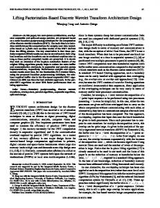
The 3D DWT can be considered as a combination of three 1D DWT in the x, y and z directions, as shown in Fig. 1. The preliminary work in the DWT processor design is to build 1D DWT modules, which are composed of high-pass and low-pass filters that perform a convolution of filter coefficients and input pixels. After a one-level of 3D discrete wavelet transform, the volume of image is decomposed into HHH, HHL, HLH, HLL, LHH, LHL, LLH and LLL signals as shown in the Fig. 1 [3]. 2.2. Lifting Scheme

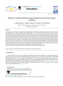
The basic idea behind the lifting scheme is very simple; try to use the correlation in the data to remove redundancy [4, 5]. First split the data into two sets (split phase) i.e., odd samples and even samples as shown in Fig. 2. Because of the assumed smoothness of the data, we predict that the odd samples have a value that is closely related to their neighboring even samples. We use N even samples to predict the value of a neighboring odd value (predict phase). With a good prediction method, the chance is high that the original odd sample is in the same range as its prediction. We calculate the difference between the odd sample and its prediction and replace the odd sample with this difference. As long as the signal is highly correlated, the newly calculated odd samples will be on the average smaller than the original one and can be represented with fewer bits. The odd half of the signal is now transformed. To transform the other half, we will have to apply the predict step on the even half as well. Because the even half is merely a sub-sampled version of the

PIERS Proceedings, Moscow, Russia, August 18–21, 2009

1570

Figure 1: One-level 3D DWT structure.

original signal, it has lost some properties that we might want to preserve. In case of images we would like to keep the intensity (mean of the samples) constant throughout different levels. The third step (update phase) updates the even samples using the newly calculated odd samples such that the desired property is preserved. Now the circle is round and we can move to the next level. We apply these three steps repeatedly on the even samples and transform each time half of the even samples, until all samples are transformed. 2.3. Rationalization of Filter Coefficients

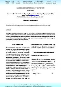
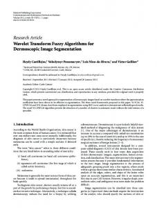
As already stated lifting scheme is one of the most efficient algorithms for the implementation of discrete wavelet transform. But one of the major shortcomings with this scheme is that the lifting coefficients obtained for the implementation of bi-orthogonal 9/7 wavelet transformation are irrational numbers [7, 8]. Hence the direct irrational coefficient implementation requires lot of hardware resources and the processing time at the cost of slight improvement in the compression performance. On the other hand, lower precision in filter coefficients results in smaller and faster hardware at the cost of compression performance. In addition to this rationalization also determines other critical hardware properties such as throughput and power consumption. Hence it is suggested that they should be optimally rationalized without much affecting the compression performance. Table 1 shows the irrational and approximated rational counterpart for 9/7 filter which are considered as a very good alternative to irrational coefficients. When these coefficients are applied to image coding, the compression performance is almost same as that of irrationalized filter coefficient implementation, while the computational complexity is reduced remarkably. The heart of 3-D DWT implementation is designing of 1-D processor which is clearly elaborated in Fig. 4. The different lifting coefficients can be easily obtained for Daubechies 9/7 filter by factorization of poly phase matrix. Fig. 3 shows the implementation of 9/7 lifting scheme. This figure is direct implementation of Fig. 2 for the required scheme. When the signal passes through various steps, it is split into three separate one dimensional transforms, the high pass component Table 1: Irrational and rational lifting coefficients for 9/7 wavelet transform.

α β γ δ ζ

Irrational value −1.5861343420. . . −0.0529801185. . . 0.8828110755. . . 0.4435068520. . . 1.1496043988. . .

Rational value −3/2 −1/16 4/5 15/32 √ 4 2/5

Progress In Electromagnetics Research Symposium Proceedings, Moscow, Russia, August 18–21, 2009 1571

Scale

High Pass Component

x [n]

Split

Update

Predict

Low Pass Scale

Component

Figure 2: The lifting scheme: Split, predict, update and scale phases. z Input X[n]

Xo

α

split

Xe

-ζ

High Pass Component

1/ζ

Low Pass Component

2

2

β

γ

δ

Figure 3: 1-D lifting scheme of daubechies 9/7 for forward wavelet DWT.

Figure 4: 3-D DWT processor architecture.

(HHH) and a low pass component (LLL). Because of sub sampling the total number of transformed coefficients is same as that of original one. These transformed coefficients are then processed by x-coordinate Processor, which have the same architecture as that of y and z-processor, to complete 3-D transformation. The bi-orthogonal 9/7 wavelet can be implemented as four lifting steps followed by scaling; requires that the following equations be implemented in hardware. x1 [2n + 1] ← x [2n + 1] + α {x [2n] + x [2n + 2]} x2 [2n] ← x [2n] + β {x1 [2n + 1] + x1 [2n − 1]} x3 [2n + 1] ← x1 [2n + 1] + γ {x2 [2n] + x2 [2n + 2]} x4 [2n] ← x2 [2n] + δ {x3 [2n + 1] + x3 [2n − 1]} x5 [2n + 1] ← 1/ζ {x3 [2n + 1]} x6 [2n] ← ζ {x4 [2n]}

(1) (2) (3) (4) (5) (6)

The original data to be filtered is denoted by x[n]; and the 1-D DWT outputs are the detail coefficients x5 [n] and approximation coefficients x6 [n]. The lifting step coefficients α, β, γ and δ and scaling coefficient ζ are constants given by Table 1. The above equations are implemented on VHDL to obtain the coefficients x5 [n] and x6 [n]. These coefficients correspond to H and L respectively. Now these coefficients are passed through the 1-D processor 3 times. Where, z-coordinate processor gives the final output as the eight subsets of original image as shown in Fig. 1. These coefficients are then stored in external memory in the form of binary file. For the multiple level of decomposition this binary file can be invoked iteratively to obtain further sublevels.

PIERS Proceedings, Moscow, Russia, August 18–21, 2009

1572

3. RESULTS AND DISCUSSION

The proposed 3-D DWT algorithm based on 9/7 Daubechies filter using lifting scheme is designed and implemented using Active-HDL Version 7.2 design tools. The entire code is written in VHDL and compilation of code is done on same simulator. The whole code is developed using structural based design to tailor the hardware utilization and delay at each step. In case of 1-D DWT, one pixel per clock cycle is taken as input. As soon as five pixels are taken as input, the x-coordinate processor (shown in Fig. 4) starts working. Although total nine pixels are required for generation of coefficient set (i.e., one high pass and one low pass) but because of applied boundary extension, the x-coordinate processor starts processing after five clock cycles. In this case, because of boundary extension, the left hand side extended (two pixel) data is same as that of right hand side. Hence only five pixels are needed to start the computation. The results of 1-D DWT are presented in Fig. 5 for clear elaboration. Fig. 6 shows quantized output of the processor which can be verified along with these waveforms (shown in Fig. 5). Both the high pass and low pass components are quantized in such a way that output is only eight bit wide. This will help in easier cascading of the y-coordinate processor and z-coordinate processor. Fig. 5 and Fig. 6 clearly show the different outputs generated by 1-D processor which are in accordance with Equations (1)–(6). The different waveforms have their names written against it. 3-D DWT is simple extension of 1-D DWT. The input data in case of 1-D DWT (x-coordinate processor), picked from image file is in binary format. Once it generates the output set of coefficients it stores the result into buffer memory. After the sufficient number of coefficients are collected the y-coordinate processor starts working and it stores its results again in another buffer memory. The similar process is also followed in the case of z-coordinate processor. The output of z-coordinate processor is the final coefficient set (i.e., high pass and low pass coefficient set). The overall memory requirement is of the order of N where N is number of pixels present in one column. This is because in the output file one line is written at a time and hence we have to collect all the coefficients in one column, which will become row when transposed, and store it in the output binary file at a time. The other modules which we have implemented in VHDL are different adders and shifters which are basic building blocks of multipliers. The different multipliers implemented are α, β, γ, δ, ζ and 1/ζ multipliers. All these codes are synthesizable individually and they are implemented via shift-add operation. The multipliers are implemented using structural design approach. These all multiplier blocks are cascaded together to obtain the overall 1-D DWT implementation. The size of input that the each multiplier accepts, and the output it generates is different for each multiplier. This size is decided according to the architecture requirement. In the whole implementation of multiplier modules, 2’s compliment is used as standard for data

Figure 5: Waveform for 1-D DWT.

Progress In Electromagnetics Research Symposium Proceedings, Moscow, Russia, August 18–21, 2009 1573

Figure 6: Waveform for 1-D DWT quantization.

representation and multiplication. Wherever it is required to divide the negative number, the number is first converted into positive number, divided, and again converted back into the negative number. This approach is adopted because it requires minimal hardware (since we have to take 2’s complement only for two times, one for converting negative number into positive number and other for converting it back into negative number after division) as compared to other implementations. Proposed 9/7 lifting scheme utilizes only 42% of the total resources available of the Spartan-II chip (50 K). The chip used for the implementation is XC2S50TQ144-5. The memory requirement for this kind of architecture and data flow is only N (i.e., the length of the column required for the storage of the DWT coefficients) for the input image size of N × N × N . The maximum clock frequency reported by the timing analysis tool is more than 100 MHz. 4. CONCLUSION

In conclusion, the proposed lifting based 3D DWT architecture can save hardware cost while being capable of high throughput. This 3D DWT processor makes it possible to map sub filters onto one Xilinx FPGA. Such a high speed processing ability is expected to offer potential for real-time 3D imaging. REFERENCES

1. Daubechies, I., “Ten lectures on wavelets,” SIAM, Philadelphia, 1992. 2. Mallat, S. G., “A theory for multiresolution signal decomposition: The wavelet representation,” IEEE Transactions on Pattern Analysis and Machine Intelligence, Vol. 11, No. 7, 674–693, July 1989. 3. Jiang, R. M. and D. Crookes, “FPGA implementation of 3D discrete wavelet transform for real-time medical imaging,” ECCTD, 519–522, August 2007. 4. Sweldens, W., “The lifting scheme: A custom-design construction of biorthogonal wavelets,” Applied and Computational Harmonic Analysis, Vol. 3, No. 2, 186–200, Article No. 15, April 1996. 5. Daubechies, I. and W. Sweldens, “Factoring wavelet transforms into lifting steps,” Journal of Fourier Analysis and Applications, Vol. 4, No. 3, 247–269, 1998. 6. Sweldens, W., “The lifting scheme: A construction of second generation wavelets,” SIAM Journal on Mathematical Analysis, Vol. 29, No. 2, 511–546, March 1998. 7. Spiliotopoulos, V., N. D. Zervas, C. E. Androulidakis, G. Anagnostopoulos, and S. Theoharis, “Quantizing the 9/7 daubechies filters coefficients for 2D DWT VLSI implementions,” Digital Signal Processing, Vol. 1, 227–231, 2002. 8. Xiong, C., S. Zheng, J. Tian, and J. Liu, “The improved lifting scheme and novel reconfigurable vlsi architecture for the 5/3 and 9/7 wavelet filters,” ICCCAS, Vol. 2, 728–732, June 2004.