The forecaster using numerical model-generated weather products can ... A
primary consideration to keep in mind is the inherent limitations of numerical
models.
9.
NUMERICAL MODELS
The forecaster using numerical model-generated weather products can benefit by acquiring some knowledge of the models and computer systems that produce the charts and data sent to the field. Each numerical model is part of a system that not only creates a forecast but also performs data assimilation, data analysis, and quality control. Many factors combine to determine the quality and usefulness of a model forecast. A primary consideration to keep in mind is the inherent limitations of numerical models in terms of resolvable spatial and time scales. For example, a model with 50 n mi (90 km) spacing between gridpoints should not be expected to forecast coastal sea breeze circulations explicitly on a scale of 5 to 10 n mi (9-18 km). Similarly, a typical polar low has a spatial scale that is near the lower limit of the current Naval Operational Global Atmospheric Predication System model's (NOGAPS T79) ability to resolve on the model grid accurately (Fig. 9-1). In such cases, the large-scale model forecast can be used to infer the presence or likelihood that a given small-scale feature does exist. A good rule of thumb is that because of computational errors in wave propagation and advection, numerical models cannot be expected to resolve features explicitly that are less than four to six grid points in extent (Ross, 1986). Small-scale features can be introduced into a model through a "bogusing" procedure. Bogusing is commonly done for tropical cyclone forecasts. Of course, features of sufficiently large scale may still be misforecast because observational data are not available or deficiencies exist in the numerical model. Numerical weather prediction relies on mathematical representation of atmospheric processes such as advection, cumulus convection, and radiative transfer. Properties of the surface, including topography, ground wetness, and surface roughness must also be numerically represented. Processes such as cumulus convection, which are too small to be resolved on the scale of the model grid spacing, are parameterized in terms of the model prognostic variables, including temperature, winds, and moisture. The methods used to parameterize physical processes can vary widely between numerical models and lead to significant differences in model forecast quality and model biases. The following discussion of Navy operational forecasting models is intended only to provide an introduction and overview of basic model characteristics.
9-1
ýS,
1'ýL
!
I 1 SECOND
I 1M MINUTE
I 1 HOUR
I 1 DAY
I I MONTH
I
I
"NOGAPS.:777 Standing waves
Ultra-long waves
wTidal
~waves
MACRO a SCALE
YiT7' )::
10,KOO0 K' M
wa'ves *
MACRO SCALE
Baroclinic
f
2,0 D00 KM MESO a SCALE
PiOne8AOSa. otral 20K0 KM
POLAR LOWS .- •
:Nocturnal
-
. .J-&lowlevel jet -. Sduall lines Inertial waves Iloud clusters[
MESO 6 SCALE
I-
-
IMtn & Lake
20 KM
disturbances IThunderstormsi Clear Air Turbulence
MESO )
SCALE
I
Urban effects I
2 K
!Tornadoes
I I
i
Io I
MICRO a SCALE
Deep convectionj Short gravyty waves 2
200
IDust I devils,
MICRO 6 SCALE
Thermals
I
I
IlWakeslI I
20 M
Plumes
Roughness
MICRO V SCALE
Turbulence
C.A.S.
CLIMATOLOGICAL :SYNOPTIC &MESOI I 1PLANETARY SCALJ I SCALE SCALE
Figure 9-1.
MICROSCALE
PROPOSED DEFINITION
Scale Definitions and Various Processes with Characteristic Time and Horizontal Scales.
9-2
9.1
Description of Fleet Numerical Models
The Fleet Numerical Oceanography Center in Monterey runs two large scale numerical models on an operational basis. These simulations are the global model NOGAPS and the regional model NORAPS (Navy Operational Regional Atmospheric Prediction System). NORAPS can be run over the polar regions, but current plans call for NOGAPS to provide primary forecast coverage of the Arctic. The operational version of NOGAPS is upgraded frequently; the description included here is accurate as of late 1989. Until 1981 FNOC ran a hemispheric gridpoint primitive equation (PE) model with a horizontal resolution of 205 n mi (= 380 km). NOGAPS 2.0 was the first FNOC global model and had a resolution of 2.4 degrees east-west and 3.0 degrees north-south. NOGAPS 3.0, installed operationally in January 1988, was the first spectral model. This version was a T47 spectral model with equivalent horizontal resolution of 2.5 degrees, equivalent to about 150 n mi (275 km) in the longitudinal direction (and east-west at the Equator). NOGAPS 3.2 became operational in September 1989 and included a significant increase in horizontal resolution-from T47 to T79 (1.5 degrees, 90 n mi or 165 kin). NOGAPS 3.2 has 18 vertical levels, and it contains a complete set of physical parameterizations, including long- and short-wave radiation and cumulus convection (Rosmond, 1989). NOGAPS 3.2 forecasts are made out to 120 hours, with quality considered equal or superior to the National Meteorological Center's global model. NOGAPS 3.2 is run on the FNOC Cyber 205, taking approximately 15 minutes per forecast day (excluding the input/output time). Planned increases in computer power may allow for an increase in resolution equivalent to 50 n mi (90 km), the current grid spacing now used in NORAPS. The following section will provide a general description of how NOGAPS performed in Arctic regions. The forecaster should be aware of model biases as well as the inherent limitations of scale in the model.
9.2
Verification of Numerical Model Forecasts
Computer forecast models are in a perpetual state of update, revision, and change. For this reason, continuous monitoring of the accuracy of the model is necessary in hopes of spotting error tendencies. While surveillance is usually performed at the center producing the forecast model, the user should still verify the model forecasts against the analyses for the area of responsibility. An evaluation of a particular model is not included in this handbook, since it would soon be outdated. Rather, a few simple guidelines are given to assist the forecaster in evaluating models. Insufficient data are a problem that forecasters must face every day. Sometimes a forecast can depend on one crucial observation from one observing station. Computer models are also highly dependent on observational data. Even in data poor areas, such as the tropic and polar regions, analyses must still be produced. Inevitably, schemes must be developed to handle these regions.
9-3
The most common method of performing an analysis of the existing atmospheric variables (e.g., temperature, moisture, pressure) employs a first guess field. This field is commonly the 6- or 12-hour model forecast from the previous model run. Observational data are interpolated to grid points and compared with the first guess value at each point. If a number of observations influence a grid point, the first guess field is essentially ignored. In data poor areas, however, the possibility remains that no observational data exist within a reasonable distance of a grid point. In such cases, the first guess field now becomes the analysis at that particular grid point. If only a limited number of observations are found, the data are blended with the first guess field to arrive at an analysis. Clearly, the first guess field can play a large role in the analysis of the current meteorological variables. Thus, a good first guess field is critical. Without observational data, the analysis field in certain areas is nearly a reproduction of the model's earlier forecast. The result is a catch-22 situation: a poor forecast leads to a poor analysis that leads to a poor forecast. The Arctic forecaster needs to be aware of this possibility. Even though a computer analysis has a low pressure center at a given location and intensity, it may only be a poor forecast from 12 hours earlier. The sources of data also need to be considered by a forecaster using a computer model. The surface and upper air observational network is fairly well established and widely known. Satellites, however, can provide large amounts of data that are usable by computer-generated analyses. This information is usually supplied in two forms: cloud track winds and vertical thickness soundings. Cloud track wind data are largely confined to the midlatitudes. They are a man-machine mixture form of data where the human determines the wind direction based on cloud motion and the computer decides on the height of the cloud based on its temperature. Vertical soundings are completely automated (i.e., no human intervention is required) and can provide large amounts of data anywhere over the globe. These data are in the form of temperature/thickness soundings for a single column, similar to that of a radiosonde. The accuracy and vertical density of the data, however, are much less than that of a radiosonde. Still, the value of these data in the Arctic region cannot be disputed. Another consideration is the time of the model forecast (i.e., 0000 GMT or 1200 GMT). Surface ships often only report during daylight hours. In the Pacific Ocean, for example, more data are available for the 0000 GMT run than for the 1200 GMT run, as seen by comparing Figs. 9-2(a) and 9-2(b). Obviously these data would have a great effect on the surface analysis in this region. Time of day is less of a problem for upper air data such as RAOBS, AIREPS, and satellite soundings. 9.2.1
Model Errors
Computer forecast models are far from perfect. While in some instances the guidance they give is very valuable, at other times they can give erroneous forecasts leading to major busts. Even in the latter situations, the information provided by the model can be useful if the error characteristics of a forecast model are known. Random observation of a model performance can often lead to incorrect assumptions about a model's behavior. For example, a low that is underforecast 7 mb by a model on a given day does not mean that all lows in all situations are underforecast by the model.
9-4
4 4727. S
I/S
Figure 9-2 (a).
Location of Surface Ship Observations in the North Pacific, 0000 GMT 18 January 1989.
Figure 9-2(b).
Location of Surface Ship Observations in the North Pacific, 1200 GMT 18 January 1989.
9-5
Rather, the model's performance must be evaluated daily over a period of time to gain an understanding of the error characteristics. Model errors fall into two classes: model tendencies and systematic errors. The former refers to similar treatment of a situation without regard to season or location. An example would be that the model deepens lows too slowly. Systematic errors refer to an error occurring in the same location and/or at the same time more than once. Knowledge of both kinds of errors can be very useful to a forecaster. 9.2.2
Model Tendencies
Figure 9-3(a) is a NOGAPS 36-hour surface pressure forecast valid 0000 GMT 27 September 1988. The verifying surface analysis is shown in Fig. 9-3(b). The model underforecasts the central pressure of the mid-North Pacific low by 18 mb. Truly, to
Figure 9-3(a).
The 36 hour Surface Pressure Forecast, 0000 GMT 27 September 1988.
9-6
determine the model's performance, the forecaster should determine if the low in question is deepening, filling, or unchanged. In this case, the low had deepened 15 mb in the previous 12 hours. The model forecasts 5 mb of deepening. Thus the initial judgment is that the model is slow in deepening the low.
Figure 9-3(b).
The Surface Pressure Analysis, 0000 GMT 27 September 1988.
9-7
To obtain a complete picture, the life cycle of the low should be charted as found in Fig. 9-4(a). Several notes should be made: 1. The model fails to predict cyclogenesis; 2. While the model correctly forecast that the low would deepen, it is too slow on the rate of deepening; 3. The model continues to deepen the low even after it began to fill; 4. The rate of filling predicted by the model is poor; and 5. The greatest error is during deepening. From this analysis, clearly, the model has some serious problems forecasting this low. Figure 9-4(b) shows a similar tracing for another low. Note that while some features are the same as those found in Fig. 9-4(a), some differences occur.
Figure 9-4(a). Forecast and Verifying Central Pressure of the 25-30 September 1988 Cyclone (see Figs. 9-3(a) and 9-3(b)).
9-8
Central Pressure of Low (mb) 15 Nov 88 Barents Sea
A
1000
I 0
990
980 970
960 nr•.
I
I
I
I
I
I
I
12Z
16/ O0Z
12Z
17/
12Z
18/
12Z
00Z
00Z
I
19/
00Z
I
12Z
I
20/
00Z
12Z
Figure 9-4(b). Forecast and Verifying Central Pressure of the 15-20 November 1988 Cyclone.
The value of such a verification is obvious. It is far too easy to jump to a conclusion to explain why the model busted a forecast. A systematic approach such as the one described yields much more correct and useful information, which can assist the user when making forecasts in the future. Another example of model tendencies is shown in the four panels of Fig. 9-5. A comparison of the 36-hour forecast for 0000 GMT 25 December 1988 (Fig. 9-5(a)) and the verifying analysis (Fig. 9-5(b)) shows that the model has done a good job forecasting the overall long wave trough-ridge pattern in the North Pacific. But the important short waves are smoothed too much and are difficult to spot on the forecast chart. This error is common in models and stems from the resolution of the model. Gridpoint spacing is often 1 to 3 degrees of latitude/longitude. Small disturbances are often poorly resolved by the gridpoints of the model and lead to poor forecasts. Figures 9-5(c) and 9-5(d) are the corresponding surface pressure forecast and verifying analysis. Although the model made a good forecast of the large-scale low, the surface troughs near 180'E and 160'E (Fig. 9-5(d)) are poorly forecast. Thus, the lack of model resolution affects both surface and upper air forecasts. The forecaster should be aware of such model tendencies since they can have a large effect on the resulting forecast of various parameters such as winds, seas, and ice movement.
9-9
Figure 9-5(a).
The 500-mb Height 36-Hour Forecast, 0000 GMT 25 December 1988.
Figure 9-5(b).
The 500-mb Height Analysis, 0000 GMT 25 December 1988.
9-10
Figure 9-5(c).
The 36 Hour Surface Pressure Forecast, 0000 GMT 25 December 1988.
Figure 9-5(d).
The Surface Pressure Analysis, 0000 GMT 25 December 1988.
9-11
9.2.3
Systematic Errors
The five panels of Fig. 9-6 show a NOGAPS 36-hour surface pressure forecast and verifying analysis. The poor forecast in the Greenland-Norway area is a common problem encountered by models. The low on the Greenland icecap is "locked-in." Figure 9-6(c) is the surface pressure analysis from 36 hours earlier (i.e., the initial field for the forecast in Fig. 9-6(a)). Note the presence of a surface low over Greenland. When a low (or high) exists over high terrain on the analysis, the feature often remains over the high terrain during the entire forecast. This result stems from problems that models have reducing pressure to sea level. The error is systematic, since it occurs in the same location time after time. Although the model leaves a fictitious low over Greenland, it correctly forecasts the true low to move northeastward to Spitsbergen and is only 2 mb in error on the central pressure. Figures 9-6(d) and 9-6(e) indicate that the model makes a good forecast of the corresponding short-wave trough. This example emphasizes the fact that the forecaster should check model output for vertical consistency. A suspicious surface low may not have any upper level justification for its existence and should thus be considered with caution.
Figure 9-6(a).
The 36 Hour Surface Pressure Forecast, 0000 GMT 3 December 1988.
9-12
Figure 9-6(b).
The Surface Pressure Analysis, 0000 GMT 3 December 1988.
Figure 9-6(c).
The Surface Pressure Analysis, 1200 GMT 1 December 1988.
9-13
Figure 9-6(d).
The 500-mb Height 36-Hour Forecast, 0000 GMT 3 December 1988.
Figure 9-6(e).
The 500-mb Height Analysis, 0000 GMT 3 December 1988.
9-14
9.3
Summary
Numerical models provide a great deal of information that can assist a forecaster. Unfortunately, the model forecasts are not always correct. It is easy to become too trusting of the computer forecasts, that is, accepting the forecasts as correct without questioning their validity. Eventually, the model has a major bust that leads to an embarrassing situation for the forecaster. A total lack of trust in models usually results. For this reason, model forecasts should be constantly scrutinized for their accuracy. A working knowledge of systematic errors and model tendencies, such as the examples given in this chapter, will help prevent a forecaster from using erroneous computer guidance that could lead to large forecast errors.
9-15