Feb 4, 2005 - in the context of Naive Bayes classification, while it is also referred to as ..... In the multinomial model, a document is an ordered sequence of ...
Databases and Information Systems Group (AG5) Max-Planck-Institute for Computer Science Saarbr¨ ucken, Germany
A Bayesian Learning Approach to Concept-Based Document Classification by Georgiana Ifrim
Supervisors Prof. Dr.-Ing. Gerhard Weikum Dipl.-Ing. Martin Theobald
A thesis submitted in conformity with the requirements for the degree of Master of Science Computer Science Department Saarland University February 2005
ii
Abstract A Bayesian Learning Approach to Concept-Based Document Classification Georgiana Ifrim Master of Science Department of Computer Science Saarland University 2005
For both classification and retrieval of natural language text documents, the standard document representation is a term vector where a term is simply a morphological normal form of the corresponding word. A potentially better approach would be to map every word onto a concept, the proper word sense, based on the word’s context in the document and an ontological knowledge-base with concept descriptions and semantic relationships among concepts. The key problem to be solved in this approach is the disambiguation of polysems, words that have multiple meanings. To this end, several approaches can be pursued at different levels of modeling and computational complexity. The simplest one is constructing feature vectors for both the word context and the potential target concepts, and using vector similarity measures to select the most suitable concept. A more refined approach would be to use supervised or semisupervised learning techniques, based on hand-annotated training data. Even more ambitiously, linguistic techniques could be used to extract a more richly annotated word context, e.g. identifying the corresponding verb or even its FrameNet class for a noun that is to be mapped onto the ontology. In this work we present a practically viable method for combining Natural Language Processing techniques such as word sense disambiguation, part of speech tagging, with Statistical Learning techniques, in order to give a better solution to the problem of Text Categorization. The goal of combining the two approaches is to achieve robustness with respect to language variations and thereby to improve classification accuracy. We systematically study the performance of the model proposed, in comparison with other approaches.
iii
iv
I hereby declare that this thesis is entirely my own work except where otherwise indicated. I have used only the resources given in the list of references.
Georgiana Ifrim February, 2005
4th
v
vi
Acknowledgements I grew up professionally during this year, I found out that research can be fun. I thank my supervisors Prof. Gerhard Weikum and Martin Theobald for showing me this approach towards work and profession. Prof. Weikum had a lot of patience during the entire process of working on my thesis, he had constantly helped and motivated me through his enthusiasm towards work well done. I thank him for investing his experience and energy in such a great way for guiding me through the entire process of working on my thesis. Martin Theobald helped me a lot in the implementation of the project, suggesting all kinds of technical tricks regarding making my implementation faster and more robust. Thank you Martin for having so much patience and for sharing your knowledge with me. When I got a bit stuck in some theoretical details, Jorg Rahnenf¨ urer helped me through fruitful discussions and by his willingness to advice me in solving statistics related problems. A great contribution to my work is due to Thomas Hofmann, who had the will and patience to read at some point some sketch of my work, and gave me very useful suggestions towards improving what I have already done. I also thank my friends, Adrian Alexa - thank you for being near me throughout one year of working hard and being almost constantly tired; Natalie Kozlova - thank you for all the implementation oriented discussions; Deepak Ajwani - thank you for all the patience and energy in correcting my terrible style of writing and for being such a good friend; Shirley Siu - thank you for offering me your friendship in difficult moments of my life. A big thanks to Kerstin Meyer Ross, the IMPRS coordinator, you were the adoptive mother of all of us - ausl¨ ander Studenten, that had no clue what should do when getting to Germany. I also thank my family and I thank God, for...my life.
vii
viii
Contents 1 Introduction 1.1 Problem Statement . . . . . . . . . . . . . . . . . . . . . . . . . . . . . . . . . 1.2 Motivation . . . . . . . . . . . . . . . . . . . . . . . . . . . . . . . . . . . . . 1.3 Contribution . . . . . . . . . . . . . . . . . . . . . . . . . . . . . . . . . . . . 2 Technical Basics 2.1 Natural Language Processing . . . . 2.1.1 Stemming . . . . . . . . . . . 2.1.2 Part of Speech Tagging . . . 2.1.3 Word Sense Disambiguation . 2.2 Text Categorization . . . . . . . . . 2.2.1 Document Representation . . 2.2.2 The Naive Bayes Classifier . 2.2.3 Concept-Based Classification
1 1 1 2
. . . . . . . .
4 4 4 5 6 9 9 10 12
3 Related Work 3.1 Concept-Based Classification . . . . . . . . . . . . . . . . . . . . . . . . . . . 3.1.1 Knowledge-Driven Approaches . . . . . . . . . . . . . . . . . . . . . . 3.1.2 Unsupervised Approaches . . . . . . . . . . . . . . . . . . . . . . . . .
14 14 14 16
4 Proposed Model 4.1 Ontological Mapping . . . . . . . . . . . . . . . 4.2 Generative Model . . . . . . . . . . . . . . . . . 4.3 Improvements of Model Parameter Estimation 4.3.1 Pruning the Parameter Space . . . . . . 4.3.2 Pre-initializing the Model Parameters . 4.4 The Full Algorithm . . . . . . . . . . . . . . . .
19 19 21 26 27 29 30
. . . . . . . .
. . . . . . . .
. . . . . . . .
. . . . . . . .
. . . . . . . .
. . . . . . . .
. . . . . . . .
. . . . . .
. . . . . . . .
. . . . . .
. . . . . . . .
. . . . . .
. . . . . . . .
. . . . . .
. . . . . . . .
. . . . . .
. . . . . . . .
. . . . . .
. . . . . . . .
. . . . . .
. . . . . . . .
. . . . . .
. . . . . . . .
. . . . . .
. . . . . . . .
. . . . . .
. . . . . . . .
. . . . . .
. . . . . . . .
. . . . . .
. . . . . . . .
. . . . . .
. . . . . . . .
. . . . . .
. . . . . . . .
. . . . . .
. . . . . . . .
. . . . . .
. . . . . .
5 Implementation
32
6 Experimental Results 6.1 Experimental Setup . . . . . . . . . . . . . . . . . . . . . . . . . . . . . . . . 6.2 Results . . . . . . . . . . . . . . . . . . . . . . . . . . . . . . . . . . . . . . . . 6.2.1 Setup 1: Baseline - Performance as a function of training set size . . . 6.2.2 Setup 2: Performance as a function of the number of features . . . . . 6.2.3 Setup 3: Similarity-Based vs. Random initialization of model parameters
40 40 42 42 47 50
7 Conclusions and Future Work
54
Bibliography
56
ix
List of Figures 2.1 2.2
Types of tagging schemes. . . . . . . . . . . . . . . . . . . . . . . . . . . . . . WordNet ontology subgraph sample. . . . . . . . . . . . . . . . . . . . . . . .
6 8
4.1
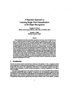
Graphical model representation of the generative model . . . . . . . . . . . .
22
5.1 5.2 5.3
Oracle storage and manipulation tables. . . . . . . . . . . . . . . . . . . . . . Data flow among developed classes. . . . . . . . . . . . . . . . . . . . . . . . . Class GenModel. . . . . . . . . . . . . . . . . . . . . . . . . . . . . . . . . . .
34 36 37
6.1 6.2 6.3 6.4 6.5 6.6 6.7 6.8
Microaveraged F1 as a function of training set size. . . . . . . . . . F1 measure for topic earn, as a function of training set size. . . . . F1 measure for topic trade, as a function of training set size. . . . . Microaveraged F1 measure as a function of the number of features. SVM classifier. Behavior in high feature spaces. . . . . . . . . . . . F1 measure for topic earn, as a function of the number of features. F1 measure for topic trade, as a function of the number of features. Similarity-based vs. random initialization. . . . . . . . . . . . . . .
43 46 46 47 48 49 49 50
x
. . . . . . . .
. . . . . . . .
. . . . . . . .
. . . . . . . .
. . . . . . . .
. . . . . . . .
List of Tables 6.1 6.2 6.3 6.4 6.5 6.6 6.7 6.8 6.9 6.10 6.11 6.12 6.13 6.14
Total number of training/test documents. . . . . . . . . . . . . . . . . . . . . Details of the classification methods at 1,000 training documents.. . . . . . . Number of concepts extracted from the ontology for various training set sizes. 50 training documents per topic. 500 features. Microaveraged F1 results. . . 50 training documents per topic. 500 features. Precision results. . . . . . . . 50 documents per topic. 500 features. Recall results. . . . . . . . . . . . . . . 50 documents per topic. 500 features. F1 measure results. . . . . . . . . . . . 200 training documents per topic. 500 features. Precision results. . . . . . . . 200 documents per topic. 500 features. Recall results. . . . . . . . . . . . . . 200 documents per topic. 500 features. F1 measure results. . . . . . . . . . . Number of concepts extracted from the ontology for various feature set sizes. Runtime results for NBayes and SVM. . . . . . . . . . . . . . . . . . . . . . . Runtime results for LatentM. . . . . . . . . . . . . . . . . . . . . . . . . . . . Runtime results for LatentMPoS. . . . . . . . . . . . . . . . . . . . . . . . . .
xi
40 43 44 44 44 44 45 45 45 45 48 51 51 52
xii
Chapter 1
Introduction
1.1
Problem Statement
Along with the continuously growing volume of information available on the Web, there is a growing interest towards better solutions for finding, filtering and organizing these resources. Text Categorization - the assignment of natural language texts to one or more predefined categories based on their content [26], is an important component in many information organization and management tasks. Its most widespread application has been for assigning subject categories to documents, to support text retrieval, routing, and filtering. Automatic text categorization can play an important role in a wide variety of more flexible, dynamic, and personalized information management tasks such as: real-time assignment of email or files into folder hierarchies; topic identification to support topic-specific processing operations; structured search and/or browsing; or finding documents that match long-term standing interests or more dynamic task-based interests. Classification technologies should be able to support category structures that are very general, consistent across individuals, and relatively static (e.g., Dewey Decimal or Library of Congress classification systems, Medical Subject Headings (MeSH), or Yahoo!’s topic hierarchy), as well as those that are more dynamic and customized to individual interests or tasks. In many contexts (Dewey, MeSH, Yahoo!, CyberPatrol), trained professionals are employed to categorize new items. This process is very time-consuming and costly, thus limiting its applicability. Consequently there is an increased interest in developing technologies for automatic text categorization [10].
1.2
Motivation
While a broad range of methods have been utilized for text categorization - Support Vector Machines, Naive Bayes, Decision Trees, virtually all these approaches use the same underlying document representation: frequencies of text terms [2], [10], where a term denotes the stem of a word or phrase in a document. This is typically called the bag-of-words representation in the context of Naive Bayes classification, while it is also referred to as the term frequency or vector space representation of documents.
1
One of the main shortcomings of term-based methods is that they largely disregard lexical semantics and, as a consequence, are not sufficiently robust with respect to variations in word usage. In order to develop better algorithms for document classification we consider that it is necessary to integrate techniques from several areas, such as Statistical Learning, Natural Language Processing, and Information Retrieval. In this work we evaluate the use of Natural Language Processing (NLP) and Information Retrieval (IR) techniques to improve Statistical Learning algorithms for text categorization, namely: • IR techniques: stop-words removal, documents as bag-of-words; • NLP techniques: stemming, part of speech tagging, word sense disambiguation (elimination of polysemy); • Statistical Learning algorithms: Bayesian classifier, Expectation Maximization. We also study some ways of exploiting the existing semantic knowledge resources, such as ontologies and thesauri (e.g. WordNet), in order to enrich the model proposed. The final goal is achieving robustness with respect to linguistic variations such as vocabulary and word choice and eventually increasing classification accuracy.
1.3
Contribution
We propose a generative model approach to text categorization that takes advantage of existing information resources (e.g. ontologies), and that combines Statistical Learning and NLP techniques in order to increase classification accuracy. The approach can be summarized in the following steps: 1. Map each word in a text document to explicit concepts; 2. Learn classification rules using the newly acquired information; 3. Interleave the two steps using a latent variable model. Different flavors of this model already exist in the literature [14] with various applications [13], [14], [15], but our work has a major contribution towards increasing robustness of the model by several techniques of pruning the parameter space and pre-initialization of the model’s parameters. We present the theoretical model and experimental results, in order to support our claims of increasing classification accuracy. We compare our approach with already existing ones: Naive Bayes classifier and Support Vector Machines, and show that our method gives better results in setups with small number of training documents. As one of the requirements of a good classification method is robustness and acceptable precision, in situations in which training data is difficult or expensive to provide, we consider our method to be a good step ahead towards solving efficiently the text categorization problem.
2
3
Chapter 2
Technical Basics
2.1
Natural Language Processing
Natural Language Processing (NLP) can be defined as the branch of information science that deals with natural language information oriented towards computer understanding, analysis, manipulation, and generation of natural language. NLP research pursues the elusive question of how we understand the meaning of a sentence or a document. What are the clues we use to understand who did what to whom, or when something happened, or what is fact and what is an assumption or prediction. While words - nouns, verbs, adjectives and adverbs - are the building blocks of meaning, it is their relationship to each other within the structure of a sentence, within a document, and within the context of what we already know about the world, that conveys the true meaning of a text. Some of the applications of NLP of special interest in our work are: • Stemming • Part of Speech Tagging • Word Sense Disambiguation In the following sections we are going to provide some basic definitions of these NLP techniques and the resources and tools used for these purposes.
2.1.1
Stemming
The technique of stemming is commonly used, especially in information retrieval tasks. In the process of stemming, various derivative forms of a word are converted to a root form of the word or stem. Root forms are then used as the terms that constitute the vocabulary for the different purposes, the most common being information retrieval. The reason for this is the belief that the different derivatives of the root form do not change the meaning of the word substantially and the similarity measure based on word stems would be more effective by ignoring differences in derivative forms [25]. In English for example, the words ”run”, ”runner” and ”running” can all be stripped down to the stem ”run” without much loss of meaning. Stemming rules can be safely used 4
when processing text in order to obtain a list of unique words. In most cases, morphological variants of words, such as singular or plural, have similar semantic interpretations and can be considered as equivalent for the purpose of IR applications. For this reason, a number of so-called stemming algorithms, or stemmers, have been developed, which attempt to reduce a word to its stem or root form. Thus, the key terms of a query or document are represented by stems rather than by the original words. This not only means that different variants of a term can be combined into a single representative form, it also reduces the dictionary size, that is, the number of distinct terms needed for representing a set of documents. A smaller dictionary size results in savings of storage space and processing time. For IR purposes, it does not usually matter whether the stems generated are genuine words or not - thus, ”computation” might be stemmed to ”comput” - provided that • different words with the same ’base meaning’ are mapped to the same form, • words with different meanings are kept separate. An algorithm which attempts to convert a word to its linguistically correct root (”compute” in this case) is sometimes called a lemmatizer. Examples of products using stemming algorithms would be search engines for intranets and digital libraries, and also thesauri and other products using NLP for the purpose of IR. Stemmers and lemmatizers also have many more applications within the field of Computational Linguistics. Some of the popular approaches to stemming are dictionary based or rule-based (Porter stemming algorithm [30]).
2.1.2
Part of Speech Tagging
Linguists group the words of a language into classes which show similar syntactic behavior, and often a typical semantic type [26]. These word classes are otherwise called syntactic or grammatical categories, but more commonly still by the traditional name Parts of Speech (PoS). Three important parts of speech are noun, verb, and adjective because they carry most of the semantic meaning in a sentence. In the process of Part of Speech Tagging, words are assigned parts of speech in order to capture generalizations about grammatically well-formed sentences, such as The noun is adjective. Determining the parts of speech of the words in a sentence can help us in identifying the syntactic structure of the sentence, and in some cases determine the pronunciation or meaning of individual words (”Did he cross the desert?” vs. ”Did he desert the army?”). There is no unique set of part-of-speech tags. Words can be grouped in different ways to capture different generalizations, and into coarser or finer categories. There are many approaches to automated part of speech tagging. In the following, we will give a brief introduction to the types of tagging schemes commonly used today [34], although no specific system will be discussed. One schema of how these approaches can be represented is given in Figure 2.1. One of the first distinctions which can be made among POS taggers is in terms of the degree of automation of the training and tagging process. The terms commonly applied to
5
this distinction are supervised vs. unsupervised.
Figure 2.1: Types of tagging schemes.
Supervised taggers typically rely on pre-tagged corpora to serve as the basis for creating any tools to be used throughout the tagging process, for example: the tagger dictionary, the word/tag frequencies, the tag sequence probabilities and/or the rule set. Unsupervised models, on the other hand, are those which do not require a pre-tagged corpus but instead use sophisticated computational methods to automatically induce word groupings (i.e. tag sets) and based on those automatic groupings, to either calculate the probabilistic information needed by stochastic taggers or to induce the context rules needed by rule-based systems. Each of these approaches has pros and cons but the discussion of them is out of the scope of this thesis.
2.1.3
Word Sense Disambiguation
The problem of Word Sense Disambiguation (WSD) can be described as follows: many words have several meanings or senses. For such words presented without context, there is thus ambiguity about how they are to be interpreted. For example, bank may be a financial institution: ”He cashed a check at the bank” or the side of a river: ”They pulled the canoe up on the bank”; chair may be a place to sit: ”He put his coat over the back of the chair and sat down” or the head of a department: ”Address your remarks to the chair”. The task of disambiguation is to determine which of the senses of an ambiguous word is invoked in a particular use of the word [26]. This is done by looking at the context of the words’ use.
Techniques Word sense disambiguation (WSD) involves the association of a given word in a text or discourse with a meaning (sense) which is distinguishable from other meanings potentially attributable to that word. The task therefore necessarily involves two steps [20]:
6
1. the determination of all the different senses for every word relevant to the text or discourse under consideration; 2. a means to assign each occurrence of a word to the appropriate sense. Much recent work on WSD relies on pre-defined senses for Step 1, including: • a list of senses such as those found in common dictionaries; • a group of features, categories, or associated words (e.g., synonyms, as in a thesaurus); • an entry in a transfer dictionary which includes translations in another language; etc. The precise definition of a sense is, however, a matter of considerable debate within the community. The variety of approaches to defining senses has raised recent concern about the comparability of various WSD techniques, and given the difficulty of the problem of sense definition, no definitive solution is likely to be found soon. However, since the earliest days of WSD work, there has been general agreement that the problems of morpho-syntactic disambiguation and sense disambiguation can be disentangled. That is, for homographs with different parts of speech (e.g., play as a verb and noun), morpho-syntactic disambiguation accomplishes sense disambiguation, and therefore (especially since the development of reliable part-of-speech taggers), WSD work has since focused largely on distinguishing senses among homographs belonging to the same syntactic category. Step 2, the assignment of words to senses, is accomplished by reliance on two major sources of information: • the context of the word to be disambiguated, in the broad sense: this includes information contained within the text or discourse in which the word appears, together with extra-linguistic information about the text such as situation, etc., • external knowledge sources, including lexical, encyclopedic resources, as well as handdevised knowledge sources, which provide data useful to associate words with senses. All disambiguation work involves matching the context of the instance of the word to be disambiguated with either information from an external knowledge source (knowledge-driven WSD), or information about the contexts of previously disambiguated instances of the word derived from corpora (data-driven or corpus-based WSD). Any of a variety of association methods is used to determine the best match between the current context and one of these sources of information, in order to assign a sense to each word occurrence. Resources Work on WSD reached a turning point in the 1980’s when large-scale lexical resources such as dictionaries, thesauri, and corpora became widely available [20]. Efforts began towards automatically extracting knowledge from these sources and, more recently, constructing largescale knowledge bases by hand. There exist two fundamental approaches to the construction of semantic lexicons: the enumerative approach, wherein senses are explicitly provided, and the generative approach, in which semantic information associated with given words is underspecified, and generation rules are used to derive precise sense information. Among enumerative lexicons, WordNet [11] is at present the best known and the most utilized resource for word sense disambiguation in 7
Figure 2.2: WordNet ontology subgraph sample.
English. It is also the resource used by us in our work. WordNet versions for several western and eastern European languages are currently under development. WordNet combines the features of many of the other resources commonly exploited in disambiguation work: it includes definitions for individual senses of words within it, as in a dictionary; it defines synsets of synonymous words representing a single lexical concept, and organizes them into a conceptual hierarchy, like a thesaurus; and it includes other links among words according to several semantic relations. Some of the relations present in the lexicon are: • hyponyms - specialization, hypernyms - generalization: e.g.a tree is a hypernym of oak, also called IS-A relation; • meronyms - part of: e.g. a branch is a meronym of tree, also called PART-OF relation; holonymy - whole of; • antonymy - opposite concepts: e.g. love is an antonym of hate. The lexicon then defines a graph, where the nodes are the different meanings and semantic relationships are the edges. The vertices are around 150,000 nouns, adverbs, verbs, or adjectives. Graph theory provides a number of indicators or measurements that characterize the structure of the graph and this type of structure is also a good way of visualizing the data stored in the lexicon. In Figure 2.2., we present a small subgraph structure for the senses of the word particle. The edges are colored to represent the type of relations among synsets: red - hypernyms, blue - hyponyms, and green - meronyms. WordNet currently provides the broadest set of lexical information in a single resource. Another, possibly more compelling reason for WordNet’s widespread use is that it is the first broad coverage lexical resource which is freely and widely available; as a result, whatever its limitations, WordNet’s sense divisions and lexical relations are likely to influence the field for years to come. WordNet is not a perfect resource for word sense disambiguation. The most frequently cited problem is the fine-grainedness of WordNet’s sense distinctions, which are often well beyond what may be needed in many language processing applications. It is not yet clear what the desired level of sense distinction should be for WSD, or if this level is even captured in WordNet’s hierarchy. Discussion within the language processing 8
community is beginning to address these issues, including the most difficult one of defining what we mean by ”sense”.
2.2
Text Categorization
2.2.1
Document Representation
In this work, we will use the standard vector representation, where each document is represented as a bag-of-words. In this model all the structure and ordering of words within the document is ignored [26]. The vector space model is one of the most widely used models for ad-hoc retrieval, mainly because of its conceptual simplicity and the appeal of the underlying metaphor of using spatial proximity for semantic proximity [26]. In this model, documents are represented as vectors in a multidimensional Euclidean space. Each dimension corresponds to a term (token). The coordinate of document d in the dimension corresponding to term t is determined by two quantities: • Term frequency T F (d, t). This is simply n(d, t), the number of times term t occurs in document d, scaled in any of a variety of ways to normalize document length [3]. For example, one may normalize the sum of term counts, in which case T F (d, t) = �n(d,t) n(d,τ ) ; τ
. The purpose is to dampen the term another way is to set T F (d, t) = maxn(d,t) τ n(d,τ ) frequency such that it represents relative degree of importance for describing the content of a document. Other functions usually� apllied to dampen term frequency are [26]: T F (d, t) = 1 + log(n(d, t)) or T F (d, t) = n(d, t). In our implementation we used the Cornell SMART system approach [23], [3]: � T F (d, t) =
0 if n(d, t) = 0 1 + log(1 + log(n(d, t))) otherwise
(2.1)
• Inverse document frequency IDF (t). Not all dimensions in the vector space are equally important. Coordinates corresponding to words such as try, have and done will be largely noisy irrespective of the content of the document. IDF seeks to scale down the coordinates of terms that occur in many documents. If D is the document collection and Dt is the set of documents containing t, then one common form of IDF weighting, also used in the SMART system and in our implementation is: IDF (t) = log
1 + |D| . |Dt |
(2.2)
If |Dt | < d, � · ||�q|| ||d||
(2.4)
Using the above formula we compute how well the occurrence of a term correlates in query and document. The cosine measure is common in manny IR systems.
2.2.2
The Naive Bayes Classifier
This section introduces the probabilistic framework and derives the Naive Bayes classifier. This is a classical frequentist approach to text analysis and categorization. In a Bayesian learning framework the assumption is that the text data was generated by a parametric model [1]. Training data is used in order to calculate Bayes optimal estimates of the model parameters. Then, equipped with these estimates, we classify new test documents by using Bayes rule to reverse the generative model and calculate the probability that a class would have generated the test document in question. Classification then becomes a simple matter of selecting the most probable class. The training data consists of a set of documents, D = {d1 , d2 , . . . , dn } where each document is labeled with a class from a set of classes C = {c1 , c2 , . . . , cm }. We assume that the data is generated by a mixture model, (parameterized by θ), with a one-to-one correspondence between mixture model components and classes. Thus, the data generation procedure for a document, di , can be understood as • select a class according to the class priors, P (cj |θ), • having the corresponding mixture components, generate a document according to its own parameters, with distribution P (di |cj ; θ). The probability of generating document di independent of its class is thus a sum of total probability over all mixture components: P (di |θ) =
|C| �
P (cj |θ) · P (di |cj ; θ)
(2.5)
j=1
Now we expand our notion of how a document is generated by an individual mixture component. In this work we approach document generation as language modeling. Thus, unlike some notions of naive Bayes in which documents are ‘events’ and the words in the document are ‘attributes’ of that event (a multi-variate Bernoulli model), we instead consider words to be ‘events’ (a multinomial model) [28]. Multinomial naive Bayes has been shown to outperform the multi-variate Bernoulli on many real-world corpora [28]. In the multinomial model, a document is an ordered sequence of word events, drawn from the same vocabulary V. We assume that the lengths of documents are independent of class. 10
We make the naive Bayes assumption: that the probability of each word event in a document is independent of the word’s context and position in the document. Thus, each document di is drawn from a multinomial distribution of words with as many independent trials as the length of di . This yields the familiar bag of words representation for documents. Define N (wt , di ) to be the count of the number of times word wt occurs in document di . Then, the probability of a document given its class is simply the multinomial distribution: |V |
P (di |cj ; θ) = P (|di |) · |di |! · Πk=1
P (wt |cj ; θ)N (wt ,di ) N (wt , di )!
(2.6)
Given the assumption about one-to-one correspondence between mixture model components and classes, and the naive Bayes assumption, the mixture model is composed of disjoint sets of for each class is composed of probabilities parameters for each class cj , and the parameter set � for each word, θwt |cj = P (wt |cj ; θ), 0 ≤ θwt |cj ≤ 1, t θwt |cj = 1. The only other parameters in the model are the class prior probabilities, written θcj = P (cj |θ). ˆ of these parameters from the training We can now calculate estimates of θ, (written θ), data. The θwt |cj estimates consist of straightforward counting of events, supplemented by smoothing with a Laplacean prior that primes each estimate with a count of one. We define P (cj |di ) ∈ {0, 1} as given by the document’s class label, then the estimate of the probability of word wt in class cj is θˆwt |cj =
�|D| 1 + i=1 N (wt , di ) · P (cj |di ) �|V | �|D| |V | + s=1 i=1 N (ws , di ) · P (cj |di )
(2.7)
The class prior parameters, θcj , are estimated by maximum-likelihood estimate - the fraction of documents in each class in the corpus: �|D| θˆcj =
i=1 P (cj |di )
|D|
.
(2.8)
Given estimates of these parameters calculated from the training documents, classification can be performed on test documents by calculating the probability of each class given the evidence of the test document, and selecting the class with the highest probability. We formulate this by applying Bayes rule: ˆ ˆ ˆ = P (cj |θ) · P (di |cj ; θ) P (cj |di ; θ) ˆ P (di |θ)
(2.9)
We can substitute in Equation 2.9 the quantities calculated in the previous equations 2.8, ˆ is the same for 2.6, 2.5, and get a decision procedure for the classifier. The quantity P (di |θ) each class, and can be discarded in the final computations. Both the mixture model and word independence assumptions are violated in practice with real-world data; however, there is empirical evidence that naive Bayes often performs well in spite of these violations [9], [12]. A variety of text representation strategies which tend to reduce independence violations have been pursued in information retrieval, including stemming, and other text normalization techniques, unsupervised term clustering, phrase formation, and feature selection.
11
2.2.3
Concept-Based Classification
We have seen in the previous section a frequentist approach to text categorization in which the main interest is in analyzing term frequencies and inferring prediction rules from the distribution of these frequencies, but so far no semantic information of natural language is exploited. The main weakness of this way of looking at world is that we are not concentrating on the underlying meaning of words in their context, but only on some statistics about their lexical representation, losing any chance of getting a better understanding of the conceptual representation of the data available, and of the process with which it has been generated. Presently there are many approaches towards overcoming this problem, which concentrate on learning the meaning of words, identifying and distinguishing between different contexts of word usage [14]. This has at least two important implications: firstly, it allows for the disambiguation of polysems, i.e., words with multiple possible meanings, and secondly, it reveals topical similarities by grouping together words that are part of a common context. As a special case this includes synonyms, i.e., words with identical or almost identical meaning. One semantics-oriented approach to text categorization is presented in [33]. This approach considers explicit concept spaces, and uses external knowledge resources such as ontologies (e.g. WordNet) to map simple terms into a semantic space. The newly extracted concepts are then used to create a concept-based feature space, that takes the meaning of words into account, and not only their lexical representation. Another direction is taken in [14] by the unsupervised technique called Probabilistic Latent Semantic Analysis (PLSA). This approach has been inspired and influenced by Latent Semantic Analysis (LSA) [8], a well-known dimension reduction technique for co-occurrence and count data, which uses a singular value decomposition (SVD) to map documents, from their standard vector space representation to a lower dimension latent semantic space. The rationale behind this is that term co-occurrence statistics can at least partially capture semantic relationships among terms and topical or thematic relationships between documents. Hence this lower-dimensional document representation may be preferable over the naive high-dimensional representation since, for example, dimensions corresponding to synonyms will ideally be conflated to a single dimension in the semantic space. Probabilistic Latent Semantic Analysis (PLSA) [14], [15], [16], is an approach that has been inspired by LSA, but instead builds upon a statistical foundation, namely a mixture model with a multinomial sampling model. The document representation obtained by PLSA allows one to deal with polysemous words and to explicitly distinguish between different meanings and different types of word usage [16]. Other semantics-oriented approaches to text analysis come from distributional clustering of words [1] and semantic kernels techniques [7], [22], and they will be discussed briefly in the next chapter.
12
13
Chapter 3
Related Work
3.1
Concept-Based Classification
Term-based representations of documents have found widespread use in information retrieval [2]. However, one of the main shortcomings of such methods is that they largely disregard semantics and, as a consequence, are not sufficiently robust with respect to variations in word usage. In the following we are going to analyze some of the approaches towards solving this problem in text categorization.
3.1.1
Knowledge-Driven Approaches
Knowledge-driven approaches start from the assumption that currently existing external knowledge sources are valuable and should be used for a better solution for the problem of text categorization. One of the resources widely used for this purpose is the WordNet ontology (thesaurus). The first approach that also inspired and partly motivated our work is the one taken in [33]. The techniques proposed in this work address mainly XML structured documents, but the technique of ontological mapping that the authors employ can be used for simple text documents as well. The way they have exploited ontological knowledge is based on the intuition that instead of using terms directly as features of a document, maybe a better idea is to map these into an ontological concept space and then learn a classifier in the mapped space. For this step they use WordNet as an underlying ontology. The resulting feature vectors refer to word sense ids that replace the original terms. This step has the potential for boosting classification by mapping terms with the same meaning onto the same word sense. An adaptation of the ontological mapping process in [33], used by us, is described in Chapter [4] in more detail. We also briefly describe their word sense disambiguation method in the following. Let w be an word that we want to map to the ontological concept space. The process of ontological mapping can be summarized as: 14
1. Query the ontology service for the possible senses of word w. 2. Let S = {s1 , s2 , . . . , sn } be the retrieved set of meanings. 3. Form a bag-of-words context around word w, from the document in which w appears. 4. Form a bag-of-words context around each of the senses si ∈ S, i ∈ {1, . . . , n} by using neighborhood information encoded in the ontology. 5. Measure the similarity of each pair of bag-of-words contexts, sim(context(w), context(si )) by cosine measure. 6. Choose the meaning of w in the specific context, to be the sense si , i ∈ {1, . . . , n} whose context has the highest similarity to context(w). Besides this WSD stage, in [33], an additional step is done regarding the enhancement of information provided by the ontology, by weighting the edges between its nodes. This additional knowledge is used in order to cover for concepts not learned by the classifier, but similar, in terms of distance in the ontology, to other learned concepts. This step is named incremental mapping and is meant for improving the classification accuracy. To handle the case of unlearned concepts, [33] defines a similarity metric between word senses of the ontological feature space, and then map the terms of a previously unseen test document to the word senses that actually appeared in the training data and are closest to the word senses onto which the test document’s terms would be mapped directly. For defining a sense-to-sense similarity metric, they pursue a pragmatic approach that exploits term correlations in natural language usage, by estimation of the dice coefficient between every two synsets in a very large text corpus. In the classification phase, the test vector is extended by finding approximate matches between the concepts in the feature space and the formerly unknown concepts of the test document. This stage identifies synonyms and replaces all terms with their disambiguated synset ids. To avoid topic drift, the search for similar concepts is limited to common hypernyms to a depth of 2 in the ontology graph. Concepts that are not connected by a common hypernym within this threshold are considered as dissimilar and obtain a similarity value of 0. The classification method applied to the feature space built as discussed above is Support Vector Machines (SVM). The hierarchical multi-class classification problem for a tree of topics, which they approach, is solved by training a number of binary SVMs, one for each topic in the tree. For each SVM, the training documents for the given topic serve as positive samples, and the training data for the tree siblings is used as negative samples. SVM computes a maximum-margin separating hyperplane between positive and negative samples in the feature space; this hyperplane then serves as the decision function for previously unseen test documents. A test document is recursively tested against all siblings of a tree level, starting with the root’s children, and assigned to all topics for which the classifier yields a positive decision (or, alternatively, only to the one with the highest positive classification confidence). The internal structure of the ontology service developed in [33] is derived from the WordNet graph and stored in a set of database relations, i.e., a relation for the nodes of the ontology graph that yield all known synsets, and a relation for each of the supported edge 15
types - hypernym, holonym, and hyponym - that connect these synsets nodes. The ontology graph provided by WordNet is enriched by edge-weights. Some part of the ontology service is also used in our implementation. In the following paragraph we discuss briefly other approaches involving external semantic knowledge resources for improving text classification accuracy [27], [18]. In [27] it is shown that the accuracy of a Naive Bayes text classifier can be improved by taking advantage of a hierarchy of classes. They use a statistical technique called shrinkage that smoothes the parameter estimates of a data-sparse child with its parent in order to obtain more robust parameter estimates. Their experiments are based on three different real-world data sets: UseNet, Yahoo and corporate webpages. A similar approach, can be found in [18]. In this work it is considered that taxonomies encode important semantic information that can be exploited in learning classifiers from labeled training data. An extension of multiclass Support Vector Machine learning is proposed, which can incorporate prior knowledge about class relationships. The latter can be encoded in the form of class attributes, similarities between classes or even a kernel function defined over the set of classes. They employ taxonomies such as the World Intellectual Property Organization (WIPO-alpha collection) and WordNet and show some experiments for the text categorization and word sense disambiguation tasks.
3.1.2
Unsupervised Approaches
We present in this section further research directions that influenced our work. In [2], [16], [15], [14] the use of concept-based document representations to supplement word- or phrasebased features is investigated. The motivation is that synonyms and polysems make the word-based representation insufficient, so a better idea would be to analyze lexical semantics. The utilized concepts are automatically extracted from documents via Probabilistic Latent Semantic Analysis. Then, the AdaBoost algorithm is used in order to combine weak hypotheses based on both types of features. AdaBoost is used to combine semantic features with term-based features because of its ability to efficiently combine heterogeneous weak hypotheses. The approach in [2] stems from a different viewpoint on handling linguistic variations. As opposed to using an explicit knowledge resource, they propose to automatically extract domain-specific concepts using an unsupervised learning stage (clustering of words with similar meaning) and then to use these learned concepts as features for supervised learning. An advantage is that the set of documents used to extract the concepts need not be labeled. This approach has three stages: • First, the unsupervised learning technique known as Probabilistic Latent Semantic Analysis (PLSA) [16] is utilized to automatically extract concepts and to represent documents in a latent concept space. • Second, weak classifiers or hypotheses are defined based on single terms as well as based on the extracted concepts. 16
• Third, multiple weak hypotheses are combined using AdaBoost, resulting in an ensemble of weak classifiers. The aspect model presented in [2], [14] is involved also in our approach, and we present it together with our modifications in Chapter 4. This latent variable model is employed in different forms and with different purposes in many areas of Information Retrieval [14], [16], [15], [17]. Other approaches to unsupervised learning of semantic similarity and text categorization also rooted in statistical learning can be found in [7], [22], [1].
17
18
Chapter 4
Proposed Model
4.1
Ontological Mapping
In the following sections we are going to present a practically viable method for exploiting linguistic resources for the disambiguation and mapping of words onto concepts, and we are going to systematically study the benefits of embedding these techniques into document classification problems. In order to solve the problem of word senses ambiguity, we would like to exploit the available knowledge resources. Along with the huge growth of the information available online on the Web and the problem of efficiently organizing and accessing it, there is also a continuous growth of the knowledge resources available: dictionaries, thesauri, annotated corpora. These resources are carefully processed and organized by professionals, and form a very good starting-point in our attempt to analyze, understand and process natural language text. This is one of the reasons for this work to use the currently available knowledge resources, specifically the WordNet ontology. The approach to trying to categorize natural language content stems from the need of better understanding and dealing with the semantics of language. We would like to go a bit further than the frequentist approach to analyzing language, and try to understand language by first analyzing its contextual meaning. As a solution to this quest, we would like first to map words in text documents to a conceptual space, to their appropriate meanings, by using a background ontology and then go further in processing this new information for achieving a better model of the given data collection. We are mostly interested in capturing synonyms - words with identical or very similar meaning and polysems - words with multiple meanings. For pursuing this, we have followed the approach in [33], [2]. In Chapter 2 we have presented WordNet as an ontology DAG of concepts c1 . . . ck where each concept has a set of synonyms: words or composite words that express the concept, a short textual description, and hypernym, hyponym, meronym or holonym edges. Let w be a word that we want to map to the ontological senses. The procedure can be summarized as follows: • Query WordNet ontology for the possible meanings of word w; for improving precision we can use part of speech annotations. This way we will only analyze senses corresponding to the PoS employed in the specific context.
19
• Let {s1 , . . . , sm } be the set of meanings associated with w. For example if we query WordNet for the word mouse we get something like: – The noun mouse has 2 senses in WordNet. 1. mouse – (any of numerous small rodents typically resembling diminutive rats having pointed snouts and small ears on elongated bodies with slender usually hairless tails) 2. mouse, computer mouse – (a hand-operated electronic device that controls the coordinates of a cursor on your computer screen as you move it around on a pad; on the bottom of the mouse is a ball that rolls on the surface of the pad; ”a mouse takes much more room than a trackball”) – The verb mouse has 2 senses in WordNet. 1. sneak, mouse, creep, steal, pussyfoot – (to go stealthily or furtively; ”..stead of sneaking around spying on the neighbor’s house”) 2. mouse – (manipulate the mouse of a computer) By taking also the synonyms of these word senses, we can form synsets for each of the word meaning. After this first step of establishing possible senses for w, we would like to know which of them is appropriate in the local context of usage. We observe w in a certain textual context, and we would like to be able to extract the corresponding meaning, by using the context information. The disambiguation technique proposed uses word statistics for a local context around both the word observed in a document and each of the possible meanings it may take. The context for the word is taken to be a window around its offset in the text document; the context around each of the possible senses is taken from the ontology: for each sense si we take its synonyms, hypernyms, hyponyms, holonyms, and siblings and their short textual descriptions, to form the context. The context around a concept in the ontology can be taken until a certain depth, depending on the amount of noise we are willing to introduce in our disambiguation process. In our implementation we used depth 2 in the ontology graph. Now for each of the candidate senses si , we compare the context around the word context(w) with context(si ) in terms of bag-of-words similarity measures. We have used the cosine similarity measure between the tf · idf vectors of context(w) and context(si ), i ∈ {1, · · · , m}. This process can either be seen as a proper word sense disambiguation step, if we take as corresponding word sense the one with the highest context similarity to the word context, or as the degree of expression of concepts into words, how words and concepts are related together and in what degree. We will come back to this second approach in the next section, when we will explain the intuitive foundation of the model proposed. We have presented in this section an example of mapping using WordNet as an underlying ontology. Any other customized ontology with a similar structure could be plugged in the model, and the process of mapping remains the same. We propose in the following a Statistical Learning approach to concept-based text categorization, enhanced with NLP preprocessing techniques so as to increase robustness of the model and thereby the classification accuracy.
20
4.2
Generative Model
In this section we introduce our framework and the theoretical model proposed. The general setup is the following: given • A document collection, D = {d1 , . . . , dr }, with known topic labels, T = {t1 , . . . , tm }, which is split into train and test data. The training collection is used to learn a classifier; the learned prediction rules are applied to assign a topic label to a new document previously unseen by the classifier. In our setup, we suppose each document to be associated with one topic label, so we exclude the case of overlapping topics. • A set of lexical features, F = {f1 , . . . , fn }, that can be observed in documents. These could be individual or composite words, pairs of adjacent words, pairs of adjacent nouns (to capture composite words), pairs of words within a bounded text window, boundedcardinality sets of words within a window, verb-noun pairs within the same sentence so as to capture subject-predicate plus predicate-object. • An ontology DAG of concepts, C = {c1 , . . . , ck }, where each concept has a set of synonyms (words or composite words that express the concept) and a short textual description, and is related to the other concepts by hypernym, hyponym, holonym edges. The goal is solving a document classification problem: for a given document d with observed features, we would like to predict P [t|d] for every topic t or find argmaxt P [t|d]. The motivation for the model presented in this section has an intuitive grounding. Consider analyzing documents categorized with a certain topic label, e.g. physics. Conceptually, this broad concept (the topic label) can be described at semantical level by a subset of more fine grained concepts, in this specific case concepts that describe lets say phenomena or structures related to physics, e.g {atom, molecule, particle, corpuscle, mote, speck}, physics, physical science, natural philosophy, etc. In turn, these finer grained concepts are expressed at the lexical level, by means of simple terms or compounds: physical science, material. We will develop a probabilistic model of the given data collection starting from the intuition given above that: • certain topics generate certain concepts: the concept {atom, molecule, particle, corpuscle, mote, speck}, as it appears in the ontology WordNet, is more probable to appear in a document labeled with topic physics than topic music; • certain concepts generate certain lexical representations of term features in documents: the concept {atom, molecule, particle, corpuscle, mote, speck} is described by many lexical representations – synonymy: e.g. particle, material, stuff - synonyms of this concept as taken from WordNet, – polysemy: depending on a certain topic, different features are associated with different concepts; e.g. for topic physics, particle might appear with the meaning:
21
Figure 4.1: Graphical model representation of the generative model
particle – (a body having finite mass and internal structure but negligible dimensions) and for topic linguistics might be used with the meaning particle – (a function word that can be used in English to form phrasal verbs) for topic linguistics. Thus, we are trying to understand how different topics are expressed at the semantic level in the training collection, and also study how this semantic world is expressed at the level of lexical features. Concepts can act as a hidden layer in between the features layer and the topics layer. Starting from the intuition given above, we wanted to formalize it by means of a statistical learning model. By pursuing this direction, we realized that we have met in the middle with a similar already existing model, the aspect model [14] developed by T. Hofmann for Probabilistic Latent Semantic Analysis. This is an unsupervised learning technique aimed at identifying and distinguishing between different contexts of word usage without recourse to a dictionary or thesaurus. Our approach stems from a supervised view, in which we use existing knowledge resources to identify and use the information needed. This way we also have the advantage of some additional information on the model, that we can use in a preprocessing step. We will analyze this point later in Section 4.3.1. Approaching the text categorization problem from a statistical learning view point comes with the advantages of a well grounded statistical theory for model fitting, model selection and complexity control [14]. The aspect model is a latent variable model for co-occurrence data which associates an unobserved variable c ∈ {c1 . . . ck } with each observation. In our case we consider an observation to be a pair (f, t), where f ∈ F is a feature (simple or compound word in this analysis) observed in some document and t ∈ T stands for a topic label. Our generative model for feature-topic co-occurrence can be thought of as: 1. select a topic t with probability P [t]; 2. pick a latent variable c with probability P [c|t], the probability that topic t generated concept c; 3. generate a feature f with probability P [f |c], the probability that concept c generated feature f . The pairs (f, t) can be directly observed, while the existence of concepts implies some process of word sense disambiguation, a mapping into a concept space, and they will be treated as latent variables. The model is based on two independence assumptions: observation pairs (f, t) are assumed to be generated independently and it is assumed that features f are conditionally 22
independent of the topics t, given the latent variable c: P [f, t|c] = P [f |c] · P [t|c]. The joint probability model is given by:
P [f, t] =
�
P [c, f, t] =
c
�
�
P [c] · P [f, t|c] =
c
P [c] · P [f |c] · P [t|c] =
c
�
P [t] · P [f |c] · P [c|t]
c
(4.1) To describe the generative process of an observation (f, t) we sum up over all the possible values that the latent variables might take P [f, t] =
�
P [c] · P [f, t|c].
(4.2)
c
The likelihood of the observed pairs (f, t) can be expressed as: L = Πf,t P [f, t]n(f,t)
(4.3)
where n(f, t) is the number of occurrences of feature f in the training set of topic t. The learning problem can be expressed now as a maximization of the observed data log-likelihood: l=
�
n(f, t) · log(P [f, t]) =
(f,t)
�
� n(f, t) · log( P [c] · P [f, t|c])
(f,t)
(4.4)
c
Due to the existence of the sum inside the logarithm direct maximization of the loglikelihood by partial derivatives is difficult. But if we knew for each pair (f, t) exactly by which of the latent variables it was generated, we could express the complete log-likelihood without a log of sums, because only one term inside the sum would be non-zero. So let us introduce indicator variables � 1 if the pair (f, t) was generated by concept c (4.5) ∆c = 0 otherwise The joint density becomes: P [f, t, ∆c ] = Πc (P [c] · P [f, t|c])∆c
(4.6)
and the complete data likelihood is: Lcomp = Πf,t P [f, t, ∆c ]n(f,t) .
(4.7)
Now we can express the complete log-likelihood of the data by: �
n(f, t) · log(P [f, t, ∆c ])
(4.8)
n(f, t) · log(Πc (P [c] · P [f, t|c])∆c )
(4.9)
lcomp =
(f,t)
lcomp =
� (f,t)
lcomp =
� (f,t)
n(f, t)
�
∆c · log(P [c] · P [f, t|c])
(4.10)
c
If we replace the missing variables ∆c by their expected values, using Jensen’s inequality we can show that the complete data log-likelihood in Equation (4.10), bounds from below the 23
incomplete log-likelihood, Equation (4.4), so we can concentrate now on the easier maximization problem, maximizing the expected complete data log-likelihood (where the expectation is taken over the missing variables ∆c ). We will estimate the expectation of these missing variables using the current values of the model parameters: P [∆c |f, t] =
Πc (P [c] · P [f, t|c])∆c P [f, t, ∆c ] = � P [f, t] c P [c] · P [f, t|c]
P [c] · P [f, t|c] = P [c|f, t] E(∆c |f, t) = P (∆c = 1|f, t) = � c P [c] · P [f, t|c] �� � n(f, t) P [c|f, t] · log(P [c] · P [f, t|c] E(lcomp ) = t
E(lcomp ) = E(lcomp ) =
�� t
f
t
f
��
f
n(f, t)
�
(4.11) (4.12) (4.13)
c
P [c|f, t] · log(P [c] · P [f |c] · P [t|c])
(4.14)
P [c|f, t] · log(P [t] · P [f |c] · P [c|t])
(4.15)
c
n(f, t)
� c
This procedure is known as the Expectation-Maximization (EM) algorithm. It is used for problems for which maximization of the likelihood is difficult, but made easier by enlarging the sample with latent data. The EM algorithm works by 2 iterative steps: • E-Step: expectation step, in which posterior probabilities are estimated for the latent variables, taking as evidence the observed data (current estimates of the model parameters); averaging the complete data log-likelihood . • M-Step: maximization step, in which the current parameters are updated based on the expected complete log-likelihood which depends on the posterior probabilities estimated in the E-Step. For calculating the probabilities of the E-step, we use Bayes’ formula:
P [c|f, t] = = = P [c|f, t] =
P [c, f, t] P [f, t] P [f |c] · P [t|c] · P [c] P [f, t|c] · P [c] � =� P [f, t|c] · P [c] c c P [f |c] · P [t|c] · P [c] P [f |c] · P [c|t] · P [t] � c P [f |c] · P [c|t] · P [t] P [f |c] · P [c|t] � c P [f |c] · P [c|t]
(4.16)
(4.17)
In the M-step, the parameters that maximize the expected complete data log-likelihood E[lc ] are calculated. So, we would now like to maximize the expected complete data log-likelihood: E[lcomp ] =
�� t
n(f, t)
�
P [c|f, t] · log(P [t] · P [f |c] · P [c|t])
(4.18)
c
f
We also have to consider the normalization constraints: � t
P [t] = 1;
�
P [f |c] = 1, ∀c;
� c
f
24
P [c|t] = 1, ∀t
(4.19)
Thus we augment E[lcomp ] with the Lagrange multipliers λ, τc , ρt : F
=
� �� {n(f, t) P [c|f, t] · log(P [t] · P [f |c] · P [c|t])} t
f
+ λ(1 −
�
c
P [t]) +
�
τc (1 −
�
c
t
P [f |c]) +
�
(4.20)
ρt (1 −
�
f
P [c|t])
c
t
We are interested in maximizing F w.r.t the following parameters: θf |c = P [f |c], θc|t = P [c|t], θt = P [t]. F
=
�� t
{n(f, t)
f
+ λ(1 −
�
� c
θt ) +
P [c|f, t] · log(θt · θf |c · θc|t )}
�
τc (1 −
�
c
t
θf |c ) +
�
ρt (1 −
t
f
(4.21) �
θc|t )
c
Setting the partial derivatives w.r.t. the parameters to zero leads us to the following equations: � n(f, t)P [c|f, t] ∂F = t − τc = 0, ∀f, ∀c (4.22) ∂θf |c θf |c � ∂F f n(f, t)P [c|f, t] = − ρt = 0, ∀t, ∀c (4.23) ∂θc|t θc|t � ∂F f,c n(f, t)P [c|f, t] = − λ = 0, ∀t (4.24) ∂θt θt We obtain: � θf |c = P [f |c] =
t n(f, t)P [c|f, t]
τc
� f
θc|t = P [c|t] = �
n(f, t)P [c|f, t] ρt
, ∀f, ∀c
(4.25)
, ∀t, ∀c
(4.26)
f,c n(f, t)P [c|f, t]
, ∀t (4.27) λ We solve for the Lagrange multipliers, taking into account the normalization constraints: θt = P [t] =
τc = ρt = λ=
�� f
t
c
f
t
f,c
�� ��
n(f, t)P [c|f, t]
(4.28)
n(f, t)P [c|f, t]
(4.29)
n(f, t)P [c|f, t]
(4.30)
So the M-step iterative equations are: � t n(f, t)P [c|f, t] P [f |c] = � � f t n(f, t)P [c|f, t]
25
(4.31)
�
f n(f, t)P [c|f, t] P [c|t] = � � c f n(f, t)P [c|f, t] � f,c n(f, t)P [c|f, t] P [t] = � � t f,c n(f, t)P [c|f, t]
(4.32) (4.33)
The E-step and M-step are iterated until some criterion is met, e.g the improvement in the likelihood is not significant or some other termination condition is met. Alternatively, one can also use the technique of early stopping - stop the algorithm when the performance on some held-out data starts decreasing, in order to avoid over-fitting the model. The way to proceed at this stage is estimating the distribution of a document d, given a topic label t, by making use of the learned features’ marginal distributions during the training process: P [d|t] = Πf ∈d P [f |t] = Πf ∈d
� P [f, t] = Πf ∈d P [f |c] · P [c|t] P [t]
(4.34)
c∈C
where P [f |c] and P [c|t] are estimated by the EM procedure as to maximize P [f, t] and implicitly P [d|t]. Naive Bayes Classifier Once we have estimates for the marginal distributions describing the generative model, we can use Bayes rule to reverse the generative model and predict which topic generated a certain document: P [t|d] =
P [d|t] · P [t] P [d|t] · P [t] =� P [d] t P [d|t] · P [t]
(4.35)
we can substitute (4.34) into (4.35) and have a decision procedure for the classifier. The hope is that the distribution that generated the given document is estimated in a more accurate way, by the means of the latent variable model. This approach to the problem of text categorization leads to a combinatorial explosion of the variable space in the model: the number of parameters is directly proportional with the cross-product of the number of features, concepts and topics. However, we can perform some pruning of this space. We will present solutions to the problem of reducing the computational complexity of this approach in the next sections.
4.3
Improvements of Model Parameter Estimation
EM faces two major problems: • a very large number of model parameters that are very sparsely represented in the observed training data, and • the possibility of converging to a local maximum of the likelihood function (i.e. not finding the global maximum). 26
For the first problem, it is desirable to prune the parameter space to reflect only meaningful and only the most important latent variables. For the second problem, it is desirable to pre-initialize the model parameters to values that are close to the global maximum of the likelihood function.
4.3.1
Pruning the Parameter Space
The parameters of our generative model are: P [f |c], P [c|t] P [c|(f, t)]. The size of the parameter space can get huge very easily, and can be very sparse due to this dimensionality problem. Our solutions to solving this problem include a couple of techniques that will be presented next. Feature Selection The feature selection process implies selecting the features that have the highest average Mutual Information with the topic variable [28]. There are two ways of interpreting this notion, depending on the underlying generative model considered. For the sake of completion we will present both approaches here. In the case of multi-variate Bernoulli model, this is done by calculating the average mutual information between the topic of a document and the absence or presence of a word in the document. We write T for a random variable over all topics, and write Wk for a random variable over the absence or presence of word wk in a document, where Wk takes values on fk ∈ {0, 1} with the following interpretation: � 1 if wk is present, (4.36) fk = 0 otherwise Average mutual information is the difference between the entropy of the topic variable, H(T ), and the entropy of the topic variable conditioned on the absence or presence of the word, H(T |Wk ): I(T ; Wk ) = H(T ) − H(T |Wk ) � P (t) · log(P (t)) + = − =
P (fk )
�
fk ∈{0,1}
t∈T
� �
� �
P (t, fk ) · log
t∈T fk ∈{0,1}
P (t, fk ) P (t) · P (fk )
(4.37) P (t|fk ) · log(P (t|fk ))
t∈T
�
where P (t), P (fk ) and P (t, fk ) are calculated by sums over all documents in the following way: • P (t) is the number of documents with topic label t divided by the total number of documents, • P (fk ) is the number of documents containing one or more occurrences of word wk divided by the total number of documents, and • P (t, fk ) is the number of documents with topic label t that also contain word wk divided by the total number of documents. 27
For the multinomial model the quantity is computed by calculating the mutual information between: 1. the topic of the document from which a word occurrence is drawn, and 2. a random variable over all word occurrences. In this model the word occurrences are the events. This calculation also uses Equation (4.37), but calculates the values of the terms by sums over word occurrences instead of over documents: • P (t) is the number of word occurrences appearing in documents with topic label t divided by the total number of word occurrences; • P (fk ) is the number of occurrences of word wk divided by the total number of word occurrences; • P (t, fk ) is the number of word occurrences of word wk that also appear in documents with topic label t, divided by the total number of word occurrences. As a preprocessing step before applying this feature selection criterion, we extract semantically significant compounds using a background dictionary (in our implementation we used WordNet), e.g. crude oil, saudi arabia, exchange market, etc. This is a further step in capturing the semantics of interesting and common language constructions, and by using knowledge resources such as dictionaries and ontologies we can reduce some of the computational complexity - many compound terms have only one meaning; e.g. exchange market as a compound has much less meanings then if analyzed separately exchange and market, so the computational overhead decreases, while also getting an increase in accuracy. After this stage we can apply the MI selection criterion in order to select the most representative terms per topic. From the implementation view point, we consider to select the same number of features per topic, so that each topic has equal chances of being represented in the training collection by its distinctive features. The tuning parameter in this step, is the number of features to be selected and learned by the classifier. Another tuning parameter concerning the features, is the context window size to be taken around a feature when computing the feature-concept similarities.
Concept Set Selection The WordNet ontology has around 150,000 concepts linked by hierarchical relations. Using the full set of concepts provided by the ontology imposes a high computational overhead combined with a high amount of noise. A better approach is to select only a subset of concepts from the ontology, such that the semantics of the training collection is reflected well in this subset. In our work we call this the candidate set of concepts. This set is selected in a preprocessing step, before running the EM algorithm in the shrunken parameter space. One way of capturing this candidate set well, is to take, for each feature, all the corresponding concepts (senses), as given by the ontology, to put all these concepts together, and to work only with this subset of concepts. The size order of this set is only of a few thousands concepts, as opposed to some hundreds thousands available in the ontology.
28
Another way of even further improving the performance of this approach, is using part of speech (PoS) annotated data, in the process of mapping to the ontology and extracting the candidate set of concepts. We took both approaches in our implementation, and compared the performance of our model with or without exploiting PoS information, and we also present experimental results comparing the two approaches. Besides increasing the robustness of the model, the pruning stage proposed reduces the computational complexity significantly.
4.3.2
Pre-initializing the Model Parameters
Our proposal for initializing the parameters of the model, after the pruning step, is to combine the learning approach with a simpler approach of mapping features to concepts and concepts to topics, based on similarity measures. For each feature f , concept c and topic t we define bag-of-words contexts con(f ), con(c), con(t). In our implementation, the context around a feature is a bag-of-words formed from a text window around the offset of f in the document. In this work the window set size was adapted to the data collection on which we ran experiments. The documents from the Reuters collection contain long sentences, on average 10 to 20 words. Based on this observations, in our implementation we used a context window of length 8. For a concept c, we define its context to be the union of texts for c, its parents, children and siblings in the ontology graph; in our implementation we take the context for a concept until depth 2 in the ontology graph, for noise reduction reasons. The context for a topic t, is defined to be the bag-of-features selected from the training collection by decreasing Mutual Information value. For our implementation we use the top 100 (compound) terms with regards to MI rank. Next, we compute sim(f, c) = sim(con(f ), con(c)) by applying cosine measure to the pairs of vectors created from the bags-of-words contexts of f and c; analogously we compute sim(c, t), we normalize all the similarities computed, and we interpret them as estimates of the probabilities P [f |c] and P [c|t]. We could also use argmaxc sim(f, c) for direct mappings of features onto concepts as a simpler “discriminative“ approach, but this approach disregards all similarity/probability values other than the one for argmaxc . In the sim(f, c) and sim(c, t) computations we only consider the (f, c) and (c, t) pairs in the already pruned parameter space. The computed values are then used for initializing EM, as a preprocessing stage, in the model fitting process. This step of pre-initialization of model parameters is targeted towards getting closer to the global maximum in the process of maximizing the likelihood function, by iterating the EM algorithm.
29
4.4
The Full Algorithm
After discussing the theoretical model and the pre-processing steps, we present in this section, the full algorithm, ready to be implemented. 1. Initialize parameters: � sim(context(f ), context(c)) ( P [f |c] = 1 ∀c) θf |c = P [f |c] = � f sim(context(f ), context(c)) f
� sim(context(c), context(t)) ( θc|t = P [c|t] = � P [c|t] = 1 ∀t) c sim(context(c), context(t)) c 2. Estimate n(f,t) = number of occurrences of feature f in topic t 3. E-step: θf |c · θc|t P [f |c] · P [c|t] P [c|f, t] = � = � c P [f |c] · P [c|t] c θf |c · θc|t 4. M-step: � t n(f, t)P [c|f, t] θf |c = P [f |c] = � � f t n(f, t)P [c|f, t] � f n(f, t)P [c|f, t] θc|t = P [c|t] = � � c f n(f, t)P [c|f, t] � f,c n(f, t)P [c|f, t] θt = P [t] = � � t f,c n(f, t)P [c|f, t] 5. Iterate until termination condition. 6. Use estimates of parameters θf |c , θc|t , θt output by EM into the classifier.
30
31
Chapter 5
Implementation In order to test and evaluate our approach we implemented the model presented in the previous chapter and ran a series of experiments on the Reuters 21578 collection [24]. The implementation consists of the following steps: 1. Documents parsing and pre-processing. The pre-processing stage involves the following actions: (a) Segmentation of the data into tokens. (b) Elimination of stop-words. (c) Stemming remaining terms. (d) Storing part of speech information for the tagged collection. In the special case of the Reuters collection, the information is stored in the form of XML files, with the natural language content in between the special set of tags: < BODY >< /BODY >. We have implemented two versions of our model: one version does not involve any Part of Speech (PoS) information and exploits the natural language text in the title and the body of each document; the second version is designed for exploiting PoS annotation tags (on the Reuters collection annotated with PoS information), and uses only the body information of each document, but not the title. The title is not exploited in this case, because it does not contain sufficiently well-formed natural language text so as to be PoS annotated with an acceptable confidence. For part of speech tagging of the Reuters collection we have used the commercial software CONNEXOR [5]. Although, this is a commercial tool, there are still many problems with the tagging process, and the mistakes in tagging the terms introduce a certain amount of noise in the model.1 In the next chapter, we describe experiments comparing the two approaches, with or without exploiting PoS. For the model which exploits PoS tags, we select only nouns and verbs as they capture most of the semantics. This action has also an impact on the computational complexity of the program, as it reduces the vocabulary size significantly. 1
One example of noise introduction is incorrectly unifying two terms into one, and reporting a new part of speech: e.g. vigurouslyresist, reported as noun, or speculationfor, reported as noun also. Another aspect concerns losing some discriminant terms: e.g. for crude oil, a highly discriminative term for the topic crude in the Reuters collection, after the tagging process crude is tagged as an adjective, oil is tagged as noun, so we lose the significant compound.
32
2. Search for compound terms as existing in the WordNet dictionary. We allow compound terms up to length three. This step reduces the computational complexity of the disambiguation process, due to the fact that a compound term is much less ambiguous then just simple terms (e.g. diesel engine, crude oil, exchange market). 3. Feature selection by computing Mutual Information (MI) with respect to a topic. The threshold on MI allows varying the number of features involved in the model. 4. Candidate concepts set selection by selecting from the WordNet ontology, concepts expressed by the features extracted in the previous step. For each feature in turn, we take all the concepts associated with that feature in the WordNet ontology, and store them in a separate set. Only these concepts are used to analyze the level of expression of the topics in the training collection. This step plays two roles: • prunes out the noise of the huge set of concepts present in the ontology. In WordNet, there are around 150.000 concepts and by our pre-selection step, we only consider some thousand of them. This step influences model robustness. • decreases the computational complexity of the implementation, by computing parameters only involving a small subset of concepts. The number of selected candidate concepts is around some thousand concepts. In this step the usage of Part of Speech information plays a very important role, not only from the precision point of view, but also from the computation point of view, because the candidate set size for the model exploiting PoS tags is in some cases, half the size of the one that does not use PoS information. But again, we also have to consider the noise introduced by the PoS tagging, which is non-negligible. Steps 4 and 5 form the stage of pruning the parameter space of the model. 5. Pre-initialization of model parameters. In this step, all the similarities between features, concepts and topics are computed and stored in the database. For the disambiguation step, we use parts of the ontology service developed in [33]. In this initialization step, the pruning of model parameters becomes very important, as we have to compute a number of parameters directly proportional to the size of the cross-product of the number of features, concepts and topics. This is not an easy computation, taking into consideration that each feature can appear many times in the training collection, and for each of these occurrences we have to compute cosine similarities between bag-of-words contexts. 6. Storing and manipulation of processed data. Data is stored in the form of Oracle tables. All the quantities computed by the algorithm and also the pre-initialization of the parameters is done via Java-Oracle communication. 7. Running the algorithm. For implementation, we have used Java 1.4.2 and Oracle 9.2.0. The tables used for storage and manipulation of the data are presented in Figure 5.1. The arrows between the tables are meant to represent common attributes among the tables, that are used in join operations. After parsing and tokenizing the data, all the interesting information is stored in the table T ERM S. We store each (compound) term, and information about its offset in the document 33
TERMS
TOPICS
+docid: number +doc_title: varchar2 +term: varchar2 +offset: number
+docid: number +topic: varchar2
MI +topic: varchar2 +term: varchar2 +MI: number
SIM_FC
SIM_CT
+feature: varchar2 +conceptid: varchar2 +sim: number
+conceptid: varchar2 +topic: varchar2 +sim: number
P_T
EM_E
+topic: varchar2 +prob: number
+conceptid: varchar2 +feature: varchar2 +topic: varchar2 +prob: number +nft: number
TF
IDF
+docid: number +feature: varchar2 +tf: number
+feature: varchar2 +idf: number
BAYES_PFT +feature: varchar2 +topic: varchar2 +prob: number
Figure 5.1: Oracle storage and manipulation tables.
in which it appears. We use this information in a later stage, when we are interested in the local context of the word. In the case of the PoS tagged collection, we encode the information about the PoS in the
34
term, by creating new terms: e.g. for the term oil which is tagged as a noun, we create a new term oil$N. This reduces storage requirement and computational effort, as we can reuse the same code and storage tables. The additional PoS information is used in the process of mapping terms onto the ontology, increasing the precision of mapping. Instead of taking all the possible senses for a term, we only take the senses corresponding to the PoS implied by the specific context: e.g. for the term trade we can find in WordNet 7 possible senses as a noun, and 5 senses as a verb. By using the PoS tags, we reduce considerably the amount of noise in the mapping stage, as we only use the senses for the PoS expressed in the specific context. The topic corresponding to each training document is stored in the table T OP ICS. By organizing the information in this manner, we provide easier access and manipulation of the data. For computing the MI of a term with respect to each topic, we only need to join the two tables, T ERM S and T OP ICS on the common attribute topic, and perform all the computations by means of SQL queries. The information stored in the MI table is then used for the feature selection step. The data stored in the T ERM S and T OP ICS tables can be used for computing frequency statistics by means of SQL statements. The SIM F C and SIM CT and P T tables are used to store information regarding the model parameters. In the table SIM F C, we store all the similarities of (feature, concept) tuples, normalize these similarities to simulate co-occurrence probabilities, and use them in the E-step of the EM algorithm. The SIM CT table plays a similar role, just that in this case we store co-occurrence probabilities for (concept, topic) tuples. In P T we store the probability of each topic, recomputed in the M-step of each iteration of EM algorithm. The changes in the parameter values in the EM iterations are handled by updating the above tables. EM E table is used for storing the conditional probabilities P [c|f, t] computed in the E-step of the EM algorithm. We store for each triplet (concept, feature, topic) the conditional probability, as well as information about the frequency of each feature in the training collection of each topic n(f, t). The T F table is used for the Naive Bayes terms-only classifier to store the parameters of the model. For each (feature, topic) tuple, we store the conditional probability calculated by frequency statistics in the training collection. T F and IDF tables are used for the SVM classifier in order to build the feature space by calculating tf · idf weights for each dimension of the vector space. For calculating these weights we have used the normalization techniques employed by the Cornell SMART system [23]. The technical details for this step have already being given in Chapter 2. For the SVM classifier, we use a linear kernel and all the other parameters use the default settings provided by the SVM Light and SVM Struct packages [32]. The BAY ES P F T table stores the conditional probabilities P [f |t] for the terms-only Naive Bayes. The parameters are calculated by Maximum Likelihood according to the theoretical basis given in Chapter 2. Storing all the requisite information in Oracle tables allows easy and fast access to the data. Instead of manipulating different data structures directly from Java, we do all the necessary processing and computations using SQL queries and use the returned results. 35
DB
DBConnections
DBUtil
Main
TablesCreator
36
Figure 5.2: Data flow among developed classes. ClassifEvaluation
SVMClassifier
BayesClassifier
GenModel
FeatureSelection
ReutersParser
DocHandler
DocParser
DatabaseBackedOntology
StemmerDriver
WordNetWrapper
In Figure 5.2 we present the main classes of the implementation and the data flow between them.
We are going to briefly explain the role of each class in Figure 5.2. • Main: This class acts as a mediator between the database and all the classifiers implemented. Pointers to the database connections are created using class DBConnections and passed to all the classes that need access to the database: DBUtil, FeatureSelection, GenModel, SVMClassifier. • DBUtil: Handles all the operations involving the database. It contains methods for creating tables, querying the database, inserting, updating, or deleting records. • ReutersParser: Parses the document collection and calls the necessary methods for processing the data. • DocHandler: Prepares the setup for extracting compound terms; handles stemming by calling the StemmerDriver class, and the storage of important information into Oracle tables, calls DocParser methods. • DocParser: Extracts natural language text from XML documents, tokenizes the text and returns (compound) terms. • DatabaseBackedOntology: Contains methods for manipulating the WordNet ontology. The classes DatabaseBackedOntology, WordNetWrapper and StemmerDriver were developed as a part of the ontology service described in [33]; besides these three classes, all the others were developed as part of this thesis. • StemmerDriver: Stemming individual terms using the Snowball stemming software [31]. • FeatureSelection: Extracts top N terms with w.r.t. their MI value, where N is a tuning parameter that controls the overfitting effects. The same feature selection criteria is used for all the methods evaluated. • GenModel: Implements the EM algorithm. In Figure 5.3 we list the main methods of this class. Class GenModel +featSel: FeatureSelection +features: String[] +topics: String[] +concepts_subset: ConceptContext[] +setWinLength(int): void +prepareCandidateConcepts(String[]): void +prepareCandidateConceptsWithPos(String[]): void +getFeatureContext(String, int, int): String[] +storeSimFC(boolean): void +storeSimCT(boolean): void +emEStep(int): void +emMStep(int): void +preparePT(): void
Figure 5.3: Class GenModel.
This class handles pruning of the parameter space and pre-initialization of model parameters; it iterates the EM algorithm until convergence. In our implementation, EM converges in 10-15 iterations. The complexity of each iteration can be analyzed in a similar way as in [14]. Each iteration requires O(N · M · K) operations, where N · M is the number of observation pairs (f, t), and K is the number of candidate concepts. This 37
can be verified by noticing that in the E-step, we compute N · M · K posterior probabilities, each of which determines exactly one re-estimation in each of the 3 equations of the M-step. • BayesClassifier: Implements a simple Naive Bayes classifier. Uses Laplace smoothing techniques. • SVMClassifier: Contains methods for building the training and test feature spaces. The files containing the tf · idf weights are fed into the SVM Light and SVM Struct software developed for multiclass classification using SVM. • ClassifEvaluation: Implements standard evaluation measures for classification problems: Precision, Recall, F1 measure, Accuracy. All the classification methods implemented are evaluated with the same measures. In the next chapter, we test and evaluate our method, in comparison with other standard classification methods - Naive Bayes and Support Vector Machines.
38
39
Chapter 6
Experimental Results
6.1
Experimental Setup
In this chapter, we provide empirical evidence that our approach of combining Natural Language Processing and Statistical Learning techniques outperforms traditional Naive Bayes and, in some setups, even the popular SVM classifier. We present experimental results on the Reuters-21578 dataset. This collection was compiled by David Lewis from the Reuters newswire in 1987. We used the “ModApte” split, that led to a corpus of 9,603 training documents and 3,299 test documents. We parsed the document collection and retained only documents belonging to one topic. This way we obtained 6,552 training documents and 2,581 test documents. Afterwards, we selected the top five categories in terms of number of training documents available: earn, acq, crude, trade, money-fx. This split the collection into approximately 5,000 files for training and 2,000 files for testing. The test set of documents is held-out, never seen by the classifier in the learning stage. Table 6.1 presents the top five categories and the maximum number of documents in the training and test sets. Category Name earn acq crude trade money-fx
Train size 2,840 1,596 253 251 206
Test size 1,083 696 121 75 87
Table 6.1: Total number of training/test documents. The classification task is to assign articles to their corresponding topics. For many categories, there is a direct correspondence between words and category labels e.g., the appearance of the crude oil term is a very good predictor of the crude category.
40
The content of the documents is expressed in natural language, so exploiting semantics by the subtle disambiguation steps can potentially boost classification accuracy. We compare our model with a Naive Bayes classifier and an SVM multiclass classifier. The Naive Bayes implementation follows the theoretical framework given in Chapter 2. For the SVM classifier, we have used the SVM Light and the SVM Struct tools, developed for multiclass classification [21], [19]. SVM multiclass is an implementation of the multi-class Support Vector Machine (SVM) described in [6]. While the optimization problem is the same as in [6], this implementation uses a different algorithm which is described in [19]. These tools (SVM Light, SVM Struct) provide a direct solution to the multiclass classification problem, without having to simulate, from the implementation side, a series of binary classification steps. We analyze and compare four classification methods: 1. LatentM - The first version of the latent generative model proposed by us that does not exploit PoS tags. 2. LatentMPoS - Our generative model, enhanced with methods for exploiting PoS information. 3. NBayes - A terms-only Naive Bayes classifier. 4. SVM - A multiclass Support Vector Machine classifier. In our experiments, we analyze the behavior of these classification methods w.r.t two parameters: • Number of training documents - we are interested in obtaining high classification accuracy, with a small number of training documents per topic; • Number of features involved in the model - we would like to study the sensitivity of the methods to the size of the feature space. All four methods use the same criteria for selecting features - Mutual Information. In order to better assess the improvements proposed by our method, we compare two approaches of model parameters pre-initialization: • Similarity-based pre-initialization of model parameters - our solution. • Random pre-initialization of model parameters - classical solution in EM-like setups. The standard way of using the EM algorithm, is to randomly initialize the model parameters, and iterate the algorithm until convergence. Due to the fact that EM tends to stop in a local maximum of the likelihood function, the standard solution is to restart EM several times, and to retain the values of the parameters that give the highest value of the likelihood. However, this solution still does not guarantee that EM will stop at a global maximum. For evaluating the classification methods, we use the following measures, commonly employed in classification and retrieval problems [26], [3]: 41
• Per topic: 1. Precision: 2. Recall:
number of correct positive predictions ; number of positive predictions
number of correct positive predictions ; number of positive examples
3. F1-measure: the harmonic mean of Precision and Recall F1 =
2 · P recision · Recall P recision + Recall
• Aggregation over all topics: 1. Microaveraged Precision: 2. Microaveraged Recall:
total number of correct positive predictions ; total number of positive predictions
total number of correct positive predictions ; total number of positive examples
3. Microaveraged F1 measure: the harmonic mean of Microaveraged Precision and Microaveraged Recall. Microaveraging makes the overall precision and recall depend most on the accuracy observed for the classes with the largest number of (positive) documents: the accuracy can be poor for classes with few positive examples without affecting the overall numbers much. Thus, microaveraged measures pay equal importance to each document [3].
6.2
Results
In this section, we study and compare the behavior of the different classification methods mentioned before. In all our experiments, we consider the same number of training documents for each topic. In the testing phase, we use all the test documents available for each category (∼2,000 test documents for all 5 categories).
6.2.1
Setup 1: Baseline - Performance as a function of training set size
As the Reuters collection has some highly discriminative terms leading to a high classification accuracy even with a fairly small vocabulary, we restrict the number of features to 500. We vary the number of training documents starting from 1 document per topic, to 200 documents per topic. 1. Figure 6.1 shows the microaveraged F1 measure for the classification methods - LatentMPoS, LatentM, NBayes and SVM - over all topics, as a function of the number of training documents. We can observe that for large enough number of training documents, our generative model involving PoS information performs better than the other two methods w.r.t the microaveraged F1 measure. In all the experiments shown in this chapter, the training sample was randomly chosen, and the plots were drawn for one such case. We didn’t average the performance of the models over many such randomly chosen training sets, due to time constraints. This fact explains the spikes in the performance curves shown as part of the experiments 42
Microaveraged F1 as a function of training set size. 95
LatentMPoS LatentM NBayes SVM
Microaveraged F1
90
85
80
75
70
5
10
25
50
75
125
250
500
750 1000
Number of training documents
Figure 6.1: Microaveraged F1 as a function of training set size.
presented in this chapter. More comprehensive experiments are planned to address this issue. For the case of 1,000 training documents, table 6.2 shows further details. This experiment provides empirical evidence to our hypothesis that by exploiting the semantics of natural language, we can decrease the amount of training documents needed for an acceptable classification accuracy. As Figure 6.1 shows, our model gets the same accuracy with 250 training documents as SVM gets by using 1,000 training documents. Training docs 1000
Concepts LatentM 4010
Concepts LatentMPoS 2301
Microavg F1 NBayes 90.7%
Microavg F1 LatentM 91.8%
Microavg F1 LatentMPoS 94.0%
Microavg F1 SVM 91.7%
Table 6.2: Details of the classification methods at 1,000 training documents.. One can argue that the performance gain of our model is due to the fact that we restrict SVM to 500 features. However, as we show later in Figure 6.5, the classification accuracy of SVM, in our case, does not increase much with increasing number of features. Table 6.3 shows some statistics regarding the number of concepts involved in our model, for both versions of our model: LatentM and LatentMPoS. We observe that the number of candidate concepts for LatentMPoS is almost half the number of concepts for LatentM, which has a direct effect on the computational complexity and also on the performance of the model.
43
Number of training documents 5 10 25 50 75 125 250 500 750 1000
Number of concepts LatentM 3531 4572 4452 4330 4339 3807 3621 3952 3882 4010
Number of concepts LatentMPoS 2088 2394 2432 2329 2358 2153 2074 2194 2306 2301
Table 6.3: Number of concepts extracted from the ontology for various training set sizes. 2. Table 6.4 shows microaveraged F1 results for 50 training documents per topic. Table 6.5, 6.6, 6.7, 6.8, 6.9, 6.10 show Precision, Recall and F1 measure results, respectively for all topics, for the case of 50 training documents per topic. Similar results for 200 training documents per topic are shown. We can observe the increase in performance w.r.t. F1 measure, while increasing the training set size. Training docs per topic 50
Concepts LatentM 3621
Concepts LatentMPoS 2074
Microavg F1 NBayes 90.0%
Microavg F1 LatentM 90.7%
Microavg F1 LatentMPoS 92.5%
Microavg F1 SVM 90.8%
Table 6.4: 50 training documents per topic. 500 features. Microaveraged F1 results. Topic acq crude earn money-fx trade
Prec NBayes 91.5% 84.6% 89.8% 92.4% 83.0%
Prec LatentM 84.2% 95.8% 94.8% 95.2% 84.2%
Prec LatentMPOS 90.5% 97.1% 93.8% 86.2% 92.3%
Prec SVM 89.9% 90.1% 92.2% 86.9% 84.8%
Table 6.5: 50 training documents per topic. 500 features. Precision results. Topic acq crude earn money-fx trade
Recall NBayes 82.5% 76.8% 98.5% 83.9% 58.6%
Recall LatentM 96.4% 64.8% 95.3% 68.9% 42.6%
Recall LatentMPOS 95.8% 63.8% 96.1% 87.2% 64.0%
Recall SVM 87.2% 76.0% 94.9% 91.9% 89.3%
Table 6.6: 50 documents per topic. 500 features. Recall results.
44
Topic acq crude earn money-fx trade
F1 NBayes 86.8% 80.5% 93.9% 87.9% 68.7%
F1 LatentM 89.9% 77.3% 95.1% 79.9% 56.6%
F1 LatentMPOS 93.1% 77.0% 95.0% 86.7% 75.5%
F1 SVM 88.5% 82.5% 93.5% 89.3% 87.0%
Table 6.7: 50 documents per topic. 500 features. F1 measure results. Topic acq crude earn money-fx trade
Prec NBayes 89.5% 90.0% 91.0% 95.1% 92.4%
Prec LatentM 85.6% 98.6% 94.9% 97.3% 90.9%
Prec LatentMPOS 91.6% 95.1% 95.9% 97.5% 83.0%
Prec SVM 89.2% 79.5% 95.4% 90.2% 84.8%
Table 6.8: 200 training documents per topic. 500 features. Precision results. Topic acq crude earn money-fx trade
Recall NBayes 82.5% 84.2% 98.2% 89.6% 65.3%
Recall LatentM 94.6% 67.5% 96.0% 83.9% 53.3%
Recall LatentMPOS 95.4% 72.2% 96.9% 89.6% 78.6%
Recall SVM 89.2% 86.7% 93.9% 85.0% 97.3%
Table 6.9: 200 documents per topic. 500 features. Recall results. Topic acq crude earn money-fx trade
F1 NBayes 85.9% 87.0% 94.5% 92.3% 76.5%
F1 LatentM 89.9% 80.2% 95.5% 90.1% 67.2%
F1 LatentMPOS 93.5% 82.1% 96.4% 93.4% 80.8%
F1 SVM 89.2% 83.0% 94.7% 87.5% 90.6%
Table 6.10: 200 documents per topic. 500 features. F1 measure results. 3. In Figure 6.2, 6.3, we present the dependency of F1 measure on the number of training documents, for the two topics: earn, trade. We chose to analyze these two topics, because of the observed discrepancy between these categories in the performance of all the methods under consideration. In spite of using the same number of training documents per topic, the classification performance w.r.t. F1 measure is highest for category earn and lowest for category trade. The category earn has the largest number of training and test documents and the performance of all the 4 methods is good on classifying documents belonging to this category. Our model outperforms Naive Bayes and SVM w.r.t. the F1 measure for this category.
45
The category trade has the smallest number of test documents, and the performance of our model in this classification task is fairly small compared to the previous category. A possible reason for this behavior is that this category is better represented with a small number of features, and in this experiment we used 500 features. A larger number of features introduces a higher amount of noise. We analyze this argument, in greater detail, in Setup 2, when studying performance dependency on the feature space size. F1 measure for topic earn. 100
LatentMPoS LatentM NBayes SVM
95
F1 measure
90
85
80
75
70
5
10
25
50
75
125
250
500
750 1000
Number of training per topic
Figure 6.2: F1 measure for topic earn, as a function of training set size.
F1 measure for topic trade. 100
LatentMPoS LatentM NBayes SVM
90
80
F1 measure
70
60
50
40
30
20
5
10
25
50
75
125
250
500
750 1000
Number of training per topic
Figure 6.3: F1 measure for topic trade, as a function of training set size.
46
6.2.2
Setup 2: Performance as a function of the number of features
In this setup, we fix the training set size to 50 documents per topic and study performance dependency on the number of features. 1. In Figure 6.4 we present microaveraged F1 measure over all the topics, as a function of the number of features. We observe that the increase in performance is in direct correlation with the feature set size. The performance increases until a certain number of features (∼ 300 - 500), and then it starts decreasing slowly, because of the increased amount of noise we introduce in the model by expanding the feature space too much. This is a known problem in applying statistical learning techniques to classification the curse of dimensionality - having less training samples than features. By increasing the number of features, we increase the complexity of the model taking the risk of overfitting - learning a particular model on the training set, which is not able to generalize and accurately predict labels of new test samples. Microavg F1 as a function of the number of features. 94
LatentMPoS LatentM NBayes SVM
92
Microaveraged F1
90
88
86
84
82 100
140
200
250
300
500
600
750
1000
Number of features
Figure 6.4: Microaveraged F1 measure as a function of the number of features. Table 6.11 shows statistics regarding the number of concepts involved in our model, at varying feature set sizes. Although in theory the SVM classifier is designed to perform well with a very large feature space and not be affected by the problem of dimensionality, we observe (as in Figure 6.5) that SVM performance w.r.t. microaveraged F1, is not better than our model performance at 500 features, even if we increase considerably the feature space size.
47
Number of features 500 600 700 800 900 1000
Number of concepts LatentM 3621 4561 5613 6200 6730 7460
Number of concepts LatentMPoS 2074 2523 3056 3422 3726 4141
Table 6.11: Number of concepts extracted from the ontology for various feature set sizes. SVM classifier. Performance as a function of the number of features. 92
SVM
91
Microaveraged F1
90
89
88
87
86
85
84 100
200
300
500
1000
1500
2000
3000
5000
10000
Number of features
Figure 6.5: SVM classifier. Behavior in high feature spaces.
2. In Figure 6.6 and Figure 6.7 we present F1 measure results for the topics earn and trade, as a function of the number of features.
48
F1 for topic earn, as a function of the number of features. 96
LatentMPoS LatentM NBayes SVM
95
94
93
F1
92
91
90
89
88
87 100
140
200
250
300
500
600
750
1000
Number of features
Figure 6.6: F1 measure for topic earn, as a function of the number of features.
F1 for topic trade, as a function of the number of features. 95
LatentMPoS LatentM NBayes SVM
90
85
80
F1
75
70
65
60
55
50
45 100
140
200
250
300
500
600
750
1000
Number of features
Figure 6.7: F1 measure for topic trade, as a function of the number of features.
We observe that the classification performance for topic trade is better for small number of features (∼ 300). Increasing the features space introduces a higher amount of noise in the task of classifying documents belonging to this category and thereby, reduces the classification accuracy.
49
6.2.3
Setup 3: Similarity-Based vs. Random initialization of model parameters
In this experimental setup, we take a different approach - we switch from analyzing the four classification methods, to assessing our model. We have proposed in this thesis a latent generative model for document classification. The solution is based on an EM algorithm, with the following artifacts so as to improve classification accuracy: 1. Pruning of model parameter space; 2. Similarity-based pre-initialization of model parameters . In this section we investigate the impact of one of this model improvements on classification accuracy - we keep the step of pruning the parameter space, but replace the similarity-based initialization by a random initialization of parameters. The purpose is analyzing whether using similarity-based initialization techniques gets us closer to the global maximum of the likelihood function. The EM algorithm is restarted 3 times with random initialization values and the classification accuracy of the random model is shown - LatentMPoSRandom in comparison to the similarity-based model - LatentMPoS. Figure 6.8 shows the microaveraged F1 measure for both approaches, at varying training set sizes; the number of features is set to 500. Microaveraged F1 as a function of training set size. 95
LatentMPos LatentMPosRandom
Microaveraged F1.
90
85
80
75
70
5
25
75
250
750
Number of training per topic
Figure 6.8: Similarity-based vs. random initialization.
We observe that w.r.t. microaveraged F1 measure, our similarity-based model performs better than the one based on random initialization. This provides empirical evidence to our hypothesis of getting closer or even at the global maximum of the likelihood by using similarity-based initialization. Still, the random-based model has a high classification accuracy; we assign this effect to the step of pruning the parameter space, that selects only important parameters in the 50
model. The EM algorithm with random initialization converges in 10-15 iterations, the speed of convergence depending on the initialization values. The impact of pruning model parameters remains to be analyzed in our future work. Running time results of our implementation Some running times of the algorithms implemented are presented in Table 6.12, 6.13, 6.14. We show the timings for varying training set sizes, and we present separately timings for our methods that involve conceptual information and for the other two methods that do not deal with semantics at all.
Table 6.12: Runtime results for NBayes and SVM.
Table 6.13: Runtime results for LatentM. We can observe that the running times of the methods are unbalanced due to the fact that allot of effort was spent already in optimizing the SVM packages - SVM Light, SVM STruct, thereby the running time of this classification method is much smaller than our methods. Due to the simplicity of a terms-only Naive Bayes classifier, the running time of this method is also much shorter than our methods. 51
Table 6.14: Runtime results for LatentMPoS.
There is a trade-off between running time vs. accuracy of the classification methods presented. Naive Bayes and SVM do not involve any information about semantics, having a gain in running time, but they lose in classification accuracy compared to our methods. In our implementation, the most time expensive step is the similarity-based initialization of model parameters. We mention that these values could be pre-computed and stored, thus drastically reducing the training times. Each EM iteration is also time consuming, but by paying this price in running time, we obtain a higher classification accuracy. As a future work our software must be optimized to reach an acceptable running time. Conclusions We have seen that the classification methods proposed by us perform better than the other approaches w.r.t. microaveraged F1 measure - 2-3% better than a Naive Bayes classifier and 1-2% better than a SVM classifier, when the number of training documents is fairly small. Thus the intuitive gain coming from analyzing language semantics is expressed over the frequency statistics (tf · idf ) used in the other two approaches. The evaluation measures used by us give equal importance to each document to be classified. Many other evaluation measures can be employed, which can show different aspects of each method’s performance. The ultimate goal of text categorization is to increase classification accuracy and at the same time reduce the need for large training set sizes (as obtaining good training collections is fairly expensive). In this chapter, we have shown that our model takes some steps ahead towards achieving this goal, giving better results than the other existing approaches, in setups with very small number of training documents per topic.
52
53
Chapter 7
Conclusions and Future Work
In this thesis, we propose a new approach to the problem of automatically classifying documents in natural language. Our solution stems from combining the techniques and knowledge from different fields: Statistical Learning, Natural language Processing and Information Retrieval. The key idea behind our work is that the semantics of natural language is valuable and it should be exploited for improving various aspects of classification problems. Given the fact that new and rich knowledge resources - like Wikipedia and WordNet are being compiled, we would like to exploit these continuously growing sources of information in achieving this goal. Although, the original knowledge sources might be very noisy, we can prune out some of the noise, and concentrate only on what we consider to be valuable semantic information. To this end, we propose to combine the idea of exploiting semantic natural language information, with techniques such as word sense disambiguation, PoS tagging, sentence tokenizing. We conduct an empirical study of the proposed methods, and show that exploiting the meaning of words, and not only their external lexical representation, does have the potential of boosting classification accuracy. In future, we want to study the behavior of the proposed techniques on other document collections, such as the Internet Movie Database (IMDB) or a real natural language collection - Wikipedia. Studying the behavior of our model on different natural language collections, will give us a better insight into the efficacy of our approach. Our ultimate goal is to understand the strengths and weaknesses of the proposed techniques, and study the benefits of applying them for document classification problems.
54
55
Bibliography [1] L. Douglas Baker, Andrew Kachites McCallum, Distributional Clustering of Words for Text Classification, Proceedings of the 21st ACM-SIGIR International Conference on Research and Development in Information Retrieval, pages 96-103, 1998. [2] Lijuan Cai, Thomas Hofmann, Text Categorization by Boosting Automatically Extracted Concepts, 26th Annual International ACM-SIGIR Conference, 2003 [3] Soumen Chakrabarti, Mining the Web: Discovering Knowledge from Hypertext Data, Morgan Kaufman Publishers, 2003. [4] Moo K. Chung, Gaussian Mixture and EM algorithm. http://www.stat.wisc.edu/∼mchung/teaching/stat471/lecture32.pdf
[5] Conexor. Part of Speech Tagger. http://www.conexor.fi/
[6] Koby Crammer, Yoram Singer, On the Algorithmic Implementation of Multiclass Kernel-based Vector Machines, Journal of Machine Learning Research 2, pages 265-292, 2001. [7] N. Cristianini, J. Shawe-Taylor, H. Lodhi, Latent semantic kernels, Proceedings 18th International Conference on Machine Learning, pages 66-73, Morgan Kaufmann Publishers, 2001. [8] Scott Deerwester, Susan T. Dumais, Richard Harshman, Indexing by Latent Semantic Analysis, Journal of the American Society of Information Science, 41(6):391-407, 1990. [9] P. Domingos, M. Pazzani, Beyond independence: Conditions for the optimality of the simple bayesian classifier, Machine Learning, 1997. [10] Susan Dumais, John Platt, David Heckerman, Inductive Learning Algorithms and Representations for Text Categorization, Proceedings of ACM-CIKM98, 1998.
56
[11] Christiane Fellbaum, WordNet: An Electronic Lexical Database, MIT Press, Cambridge, 1999. http://www.cogsci.princeton.edu/∼wn/gloss.shtml
[12] Jerome H. Friedman, On bias, variance, 0/1 - loss and the curse of dimensionality, Data Mining and Knowledge Discovery 1, pages 55-77, 1997. [13] Thomas Hofmann, Jan Puzicha, Statistical Models for Co-occurrence Data, MIT Press, Cambridge, 1998 [14] Thomas Hofmann, Unsupervised Learning by Probabilistic Latent Semantic Analysis, Kluwer Academic Publishers, 2001. [15] Thomas Hofmann, Probabilistic Latent Semantic Indexing, Proceedings of the 22nd ACM-SIGIR International Conference on Research and Development in Information Retrieval, pages 50-57, 1999. [16] Thomas Hofmann, Probabilistic Latent Semantic Analysis, Uncertainty in Artificial Intelligence, 1999. [17] Thomas Hofmann, Learning the Similarity of Documents: An Information-Geometric Approach to Document Retrieval and Categorization, Advances in Neural Information Processing Systems, volume 12, MIT Press, Cambridge, 2000. [18] Thomas Hofmann, Lijuan Cai, Massimiliano Ciaramita, Learning with Taxonomies: Classifying Documents and Words, Advances in Neural Information Processing Systems, 2003. [19] Ioannis Tsochantaridis, Thomas Hoffman, Thorsten Joachims, Yasemin Altun, Support Vector machine Learning for Interdependent and Structured Output Spaces, Proceedings of the 21st International Conference on Machine Learning, 2004. [20] Nancy Ide, Jean V´eronis, Word Sense Disambiguation: The State of the Art, Computational Linguistics, 1998. [21] T. Joachims, Text categorization with support vector machines: learning with many relevant features, Proceedings 10th European Conference on Machine Learning, pages 137-142, 1998. [22] Jaz Kandola, John Shawe-Taylor, Nello Cristianini, Learning Semantic Similarity, Advances in Neural Information Processing Systems, 2002.
57
[23] Wessel Kraaij, Variations on Language Modelling for Information Retrieval, Centre for Telematics and Information Technology, PhD. Thesis, The Netherlands, 2004. [24] David Lewis, Reuters-21578 dataset, http://www.daviddlewis.com/resources/testcollections/reuters21578/
[25] Milind Mahajan, Doug Beeferman1, X. D. Huang, Improved Topic-Dependent Language Modelling using Information Retrieval Techniques, IEEE International Conference On Acoustic, Speech, and Signal Processing, 1999. [26] Christopher D.Manning, Hinrich Sch¨ utze, Foundations of Statistical Natural Language Processing, MIT Press, Cambridge, 2000. [27] Andrew McCAllum, Ronald Rosenfeld, Tom Mitchell, Andrew Y. Ng, Improving Text Classification by Shrinkage in a Hierarchy of Classes, International Conference on Machine Learning, 1998. [28] Andrew McCallum, Kamal Nigam, A Comparison of Event Models for Naive Bayes Text Classification, AAAI-98 Workshop on “Learning for Text Categorization”, 1998. [29] Kamal Nigam, Andrew Kachites McCallum, Sebastian Thrun, Tom Mitchell, Text Classification from Labeled and Unlabeled Documents using EM, Kluwer Academic Publishers, 1999. [30] Porter Stemmer. http://www.tartarus.org/∼martin/PorterStemmer
[31] Snowball Stemmer. http://snowball.tartarus.org/
[32] SVM Light. http://svmlight.joachims.org/
[33] Martin Theobald, Ralf Schenkel, Gerhard Weikum, Exploiting Structure, Annotation, and Ontological Knowledge for Automatic Classification of XML Data, Sixth International Workshop on the Web and Databases, 2003. [34] Linda Van Guilder, Automated Part of Speech Tagging: A Brief Overview, Georgetown University, LING361, 1995. http://www.georgetown.edu/faculty/ballc/ling361/tagging overview.html
58